Multichannel Speech Separation and Enhancement Using the Convolutive Transfer Function

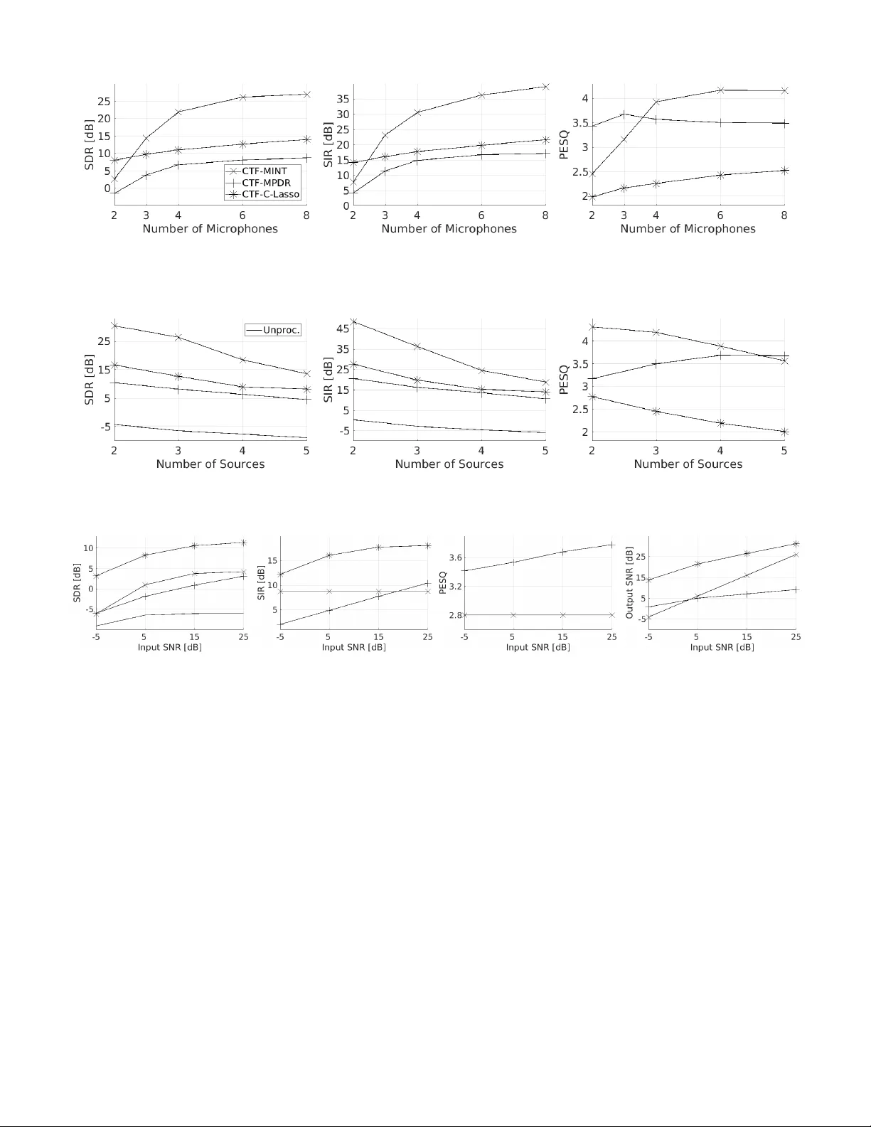
1 Multichannel Speech Separation and Enhancement Using the Con v oluti v e T ransfer Function Xiaofei Li, Laurent Girin, Sharon Gannot and Radu Horaud Abstract —This paper addresses the pr oblem of speech separa- tion and enhancement from multichannel con volutiv e and noisy mixtures, assuming known mixing filters . W e propose to perform the speech separation and enhancement task in the short- time Fourier transform domain, using the con volutive transfer function (CTF) approximation. Compared to time-domain filters, CTF has much less taps, consequently it has less near-common zeros among channels and less computational complexity . The work proposes three speech-source recov ery methods, namely: i) the multichannel in verse filtering method, i.e. the multiple input/output in verse theorem (MINT), is exploited in the CTF domain, and for the multi-source case, ii) a beamforming-like multichannel in verse filtering method applying single source MINT and using power minimization, which is suitable whenever the source CTFs are not all known, and iii) a constrained Lasso method, where the sources are reco vered by minimizing the ` 1 - norm to impose their spectral sparsity , with the constraint that the ` 2 -norm fitting cost, between the microphone signals and the mixing model involving the unknown source signals, is less than a tolerance. The noise can be reduced by setting a tolerance onto the noise power . Experiments under various acoustic conditions are carried out to evaluate the three proposed methods. The comparison between them as well as with the baseline methods is pr esented. Index T erms —A udio source separation, speech enhancement, short-time Fourier transform, con volutive transfer function, MINT , Lasso optimization I . I N T RO D U C T I O N Speech recordings in the real world consist of the conv olu- tiv e images of multiple audio sources and some additiv e noise. A con voluti ve image is the conv olution between the source signal and the room impulse response (RIR), which is also called mixing filter in the multisource context. Correspond- ingly , the distortions on the source signals, i.e. interfering speakers, reverberations and additive noise, heavily deteriorate the speech intelligibility for both human listening and machine recognition. This work aims to suppress these distortions, in other words, to recov er the respectiv e source signals from the multichannel recordings. In general, suppressing interfering speakers, reverberations and noise are respectiv ely refered to source separation, derev erberation and noise reduction. Each of which is a difficult task, that attracts lots of research atten- tions. In the microphone recordings, there are three unknown terms, i.e. source signals, mixing filters, and noise. Thence, the X. Li and R. Horaud are with INRIA Grenoble Rh ˆ one-Alpes, Montbonnot Saint-Martin, France. L. Girin is with GIPSA-lab and with Univ . Grenoble Alpes, Saint-Martin d’H ` eres, France. Sharon Gannot is with Bar Ilan University , Faculty of Engineering, Israel. This work was supported by the ERC Advanced Grant VHIA #340113. problem is often split into two subproblems i) identification of mixing filters and noise statistics, and ii) estimation of the source signals. This work focuses on the problem of speech source estimation assuming that the mixing filters, and possibly the noise statistics, are either known or their estimates are av ailable. Most con voluti ve source separation and speech enhance- ment techniques are designed in the short time Fourier trans- form (STFT) domain. In this domain, the conv olutiv e process is usually approximated at each time-frequency (TF) bin by a product between the source STFT coefficient and the Fourier transform of the mixing filter . This assumption is called the multiplicativ e transfer function (MTF) approximation [1], or the narrowband approximation, and the frequenc y domain mixing filter is called the acoustic transfer function (A TF). Based on the kno wn A TFs, or the respective relativ e transfer functions (R TFs) [2], [3], the beamforming techniques are widely used for multichannel source separation and speech enhancement, such as the minimum variance/po wer distortion- less response (MVDR/MPDR) beamformer , and the linearly constrained minimum v ariance/power (LCMV/LCMP) beam- former [2], [4]. Moreover , the sparsity of the audio signals in the TF domain can be utilized. Based on this property , the binary masking [5], [6] and the ` 1 -norm minimization [7] approaches have been applied for source separation. For more examples of MTF-based techniques, please refer to a comprehensiv e revie w [8] and references therein. The narrowband assumption is theoretically valid only if the length of the mixing filters is small relati ve to the length of the STFT windo w . In practice, this is very rarely the case, ev en for moderately rev erberant en vironments, since the STFT window is limited to assume local stationarity of audio signals. Hence the narrowband assumption fundamentally hamper the speech enhancement performance, and this becomes critical for strongly reverberant environments. T o av oid the limitation of narrowband assumption, several source separation methods based on the time-domain representation of mixing filters hav e been proposed. In the wide-band Lasso method [9], the source signals are estimated by minimizing an ` 2 -norm fitting cost between the microphone signals and the mixing model inv olving the unknown source signals, in which the exact time-domain (wide-band) source-filter conv olution is used. Importantly , the ` 1 -norm of the STFT -domain source signals is added to the fitting cost as a regularization term to impose the spectral sparsity of the source spectra. In the presence of additi ve noise, the ` 1 -norm regularization is able to reduce the noise in the recov ered source signals. Ho wever , the regularization factor is difficult to set ev en if the noise 2 power is known. T o overcome this, a more flexible scheme is proposed in [10] that relaxes the ` 2 -norm fitting cost to the noise lev el and minimizes the ` 1 -norm. In addition, a reweighting approach is also proposed in [10] to approximate the ` 0 -norm. In the family of multichannel in verse filtering or multichannel equalization, an in verse filter is estimated with respect to the kno wn mixing filters, and applied to the microphone signals, preserving the desired source and suppressing the interfering sources. The multiple-input/output in verse theorem (MINT) method [11] was first proposed for this aim, which howe ver is sensiti ve to RIR perturbations (misalignment / estimation error) and to microphone noise. T o improv e the robustness of MINT to RIR perturbations, many techniques have been proposed, preserving not only the direct- path impulse response but also the early reflections, such as channel shortening [12], infinity- and p -norm optimization- based channel shortening/reshaping [13], partial MINT [14], [15], etc. In addition, the energy of the in verse filter was used in [16] as a regularization term to a void the amplification of filter perturbations and microphone noise. In [17], a two- stage method was proposed, that first conv erts a multiple- input multiple-output (MIMO) system to multiple single-input multiple-output (SIMO) systems for source separation, and then applies in verse filtering for derev erberation. The wide-band models mentioned above are all performed in the time domain. The time-domain con volution problem can be transformed to the subband domain, which provides sev eral benefits i) the original problem is split into subproblems, and each subproblem has a smaller data size and thus a smaller computational complexity , ii) the subband mixing filters are shorter than the time-domain filters, thence are likely to have less near-common zeros among microphones, which benefits both the filter identification and the multichannel equalization, ev en if the former is be yond the scope of this work, and iii) in the TF domain, the sparsity of the speech signal can be more easily exploited. Se veral v ariants of subband MINT were proposed based on filter banks [18], [19], [20], [21], [22]. The ke y issues in the filter-bank design are i) the time- domain RIRs should be well approximated in the subband domain, and ii) the frequency response of each filter-bank should be fully excited, i.e. should not in volv e the frequency components with the magnitude close to zero. Otherwise, these components are common to all channels, and are problematic in the MINT application. T o satisfy the second condition, the filter-bank is either critically sampled [18], [19], which suffers from frequency aliasing, or has a flat-top frequency response [20], [21], [22], which may suffer from time aliasing. Generally speaking, the STFT transform is more preferable in the sense that most of the acoustic algorithms in the current literature are performed in this domain. T o represent the time- domain con volution in the STFT domain, especially for the long filter case, cross-band filters were introduced in [23]. T o simplify the analysis, the con voluti ve transfer function (CTF) approximation is further adopted in [24], [25] only using the band-to-band con volution and ignoring the cross- band filters. In [25], CTF is integrated into the generalized sidelobe canceler beamformer . In our previous works [26] and [27], blindly estimated CTF , specifically its direct-path part, was used for localizing single speaker and multiple speakers, respectiv ely . In [28], a CTF-Lasso method was proposed following the spirit of the wide-band Lasso [9]. Sev eral probabilistic techniques hav e also been proposed for wide-band source separation via maximizing the likelihood of a generativ e model. V ariational Expectation-Maximization (EM) algorithms are proposed in [29] and [30] based on the time-domain con volution and in [31] based on cross-band filters. CTF-based EM algorithms are proposed in [32] and [33] for single source derev erberation and source separation, respectiv ely . These EM algorithms iterativ ely estimate the mixing filters and the sources, and intrinsically require a fairly good initialization for both filters and sources. In this work, we propose the follo wing three source reco very methods in the standard ov ersampled STFT domain using the CTF approximation: • All the above-mentioned improved MINT methods are proposed for single source derev erberation. The multi- source case has been rarely studied, ev en if the multi- source MINT was presented in the original paper [11]. W e propose a CTF-based multisource MINT method for both source separation and dere verberation. The o versampled STFT does not suffer from both frequency aliasing and time aliasing. Howe ver , the STFT window is not flat-top, namely the subband signals and filters ha ve a frequency region with a magnitude close to zero, which is common to all channels. T o overcome this problem, instead of using the con ventional impulse function as the target of the in verse filtering, we propose a new target, which has a frequency response corresponding to the STFT window . In addition, a filter ener gy re gularization is adopted following [16] to improve the robustness of in verse filtering. • For situations where the CTFs of the sources are not all av ailable, we propose a beamforming-like in verse filtering method. The in verse filters are designed i) to preserve one source with kno wn CTFs based on single source MINT , and ii) to minimize the overall po wer of the in verse filtering output, and thus suppress the interfering sources and noise. This method shares a similar spirit with the MPDR beamformer . • T o ov ercome the drawback of the CTF-Lasso method [28], namely that the regularization factor is difficult to set with respect to the noise level, following the spirit of [10], we propose to reco ver the source signals by minimizing the ` 1 -norm of the source spectra with the constraint that the ` 2 -norm fitting cost is less than a tol- erance. The setting of the tolerance is studied. In addition, a complex-v alued pr oximal splitting algorithm [34], [35] is in vestigated to solve the optimization problem. The remainder of this paper is organized as follows. The problem is formulated based on CTF in Section II. The two multichannel in verse filtering methods are proposed in Section III. The improved CTF-Lasso method is proposed 3 in Section IV. Experiments are presented in Section V. Sec- tion VI concludes the work. I I . C T F - BA S E D P R OB L E M F O R M U L A T I O N In the time domain, we consider a multichannel conv olutiv e mixture with J sources and I microphones, x i ( n ) = J X j =1 a i,j ( n ) ? s j ( n ) + e i ( n ) , (1) where n is the time index, and i = 1 , . . . , I , I ≥ 2 and j = 1 , . . . , J, J ≥ 2 are respecti vely the indices of the microphones and the sources. The signals x i ( n ) , s j ( n ) and e i ( n ) are microphone signals, source signals, and noise signals, respectiv ely . Here ? denotes con volution, and a i,j ( n ) is the RIR relating the j -th source to the i -th microphone. Note that the relation between I and J is not specified here, and this will be discussed afterwards with respect to the proposed methods. The noise signals e i ( n ) are uncorrelated with the source signals, and could be spatially uncorrelated, diffuse, or directional. The goal of this paper is to recover the multiple source signals from the microphone signals, giv en the RIRs and the noise PSDs. The RIRs and noise PSDs could be blindly estimated from the microphone signals, and the estimated values generally suffer from disturbances, which are not trivial but beyond the scope of this work. Overall, the multi-source recov ery problem implies that source separation, dereverbera- tion, and noise reduction are conducted simultaneously . A. Con volutive T ransfer Function In this section, the time-domain con volution is transformed into the STFT -domain CTF con volution. T o simplify the expo- sition, we consider, for the meantime, the noise free situation with only one microphone and one source: x ( n ) = a ( n ) ? s ( n ) , where the source and microphone indices are omitted. The STFT representation of the microphone signal x ( n ) is x p,k = + ∞ X n = −∞ x ( n ) ˜ w ( n − pD ) e − j 2 π N k ( n − pD ) , (2) where p and k denote the frame index and the frequenc y index, respectively . ˜ w ( n ) is the STFT analysis window , and N and D denote the frame (window) length, and the frame step, respectiv ely . In the filter bank interpretation, the analysis window is considered as the low-pass filter , and D as the decimation factor . The cross-band filter model [23] consists in representing the STFT coef ficient x p,k as a summation over multiple con volutions (between the STFT -domain source signal s p,k and filter a p,k,k 0 ) across frequency bins. Mathematically , the linear time in v ariant system can be written in the STFT domain as x p,k = N − 1 X k 0 =0 X p 0 s p − p 0 ,k 0 a p 0 ,k,k 0 , (3) If D < N , then a p 0 ,k,k 0 is non-causal, with d N/D e − 1 non- causal coefficients, where d·e denotes the ceiling function. The number of causal filter coefficients is related to the rev erberation time. For notational simplicity , let the filter inde x p 0 be in [0 , L a − 1] , with L a being the filter length, i.e. the non-causal coefficients are shifted to the causal part, which only leads to a constant shift of the frame index of the source signal. Let w ( n ) denote the STFT synthesis window . The STFT -domain impulse response a p 0 ,k,k 0 is related to the time- domain impulse response a ( n ) by: a p 0 ,k,k 0 = ( a ( n ) ? ζ k,k 0 ( n )) | n = p 0 D , (4) which represents the con volution with respect to the time inde x n ev aluated at frame steps, with ζ k,k 0 ( n ) = e j 2 π N k 0 n + ∞ X m = −∞ ˜ w ( m ) w ( n + m ) e − j 2 π N m ( k − k 0 ) . T o simplify the analysis, we consider the CTF approximation, i.e., only band-to-band filters with k = k 0 are considered: x p,k ≈ X L a − 1 p 0 =0 s p − p 0 ,k a p 0 ,k = s p,k ? a p,k . (5) B. STFT Domain Mixing Model Based on the CTF approximation, we can obtain the STFT -domain mixing model corresponding to the time-domain model (1), x i p = J X j =1 a i,j p ? s j p + e i p , (6) Note that here (and hereafter) the frequenc y index k is omitted, unless it is necessary . Since the proposed methods are applied frequency-wise. Let p ∈ [1 , P ] and p ∈ [0 , L a − 1] denote the frame indices of the microphone signals and the CTFs respectiv ely . The goal of this work is to recover the STFT coefficients of the source signals, i.e. s j p , and then applying the inv erse STFT to obtain an estimation of the time-domain source signals. I I I . M U LTI C H A N N E L I N V E R S E F I LT E R I N G The multichannel inv erse filtering method is based on the MINT method. In this section, we propose two MINT -based methods in the CTF domain for the multisource case. A. Pr oblem F ormulation for In verse F iltering Define the CTF-domain in verse filters as h i p with i = 1 , . . . , I and p = 0 , . . . , L h − 1 , where L h denotes the length of the in verse filters. The output of the inv erse filtering is y p = I X i =1 h i p ? x i p = J X j =1 s j p ? I X i =1 h i p ? a i,j p ! + I X i =1 h i p ? e i p , (7) 4 which comprises the mixture of the inv erse filtered sources and the in verse filtered noise. T o facilitate the analysis, we denote the con volution in vec- tor form. W e define the con volution matrix for the microphone signal x i p as: X i =                x i 1 0 · · · 0 x i 2 x i 1 . . . . . . . . . . . . . . . . . . x i P . . . . . . 0 0 x i P . . . . . . . . . . . . . . . . . . 0 · · · 0 x i P                ∈ C ( P + L h − 1) × L h , (8) and the vector of filter h i p as h i = [ h i 0 , . . . , h i p , . . . , h i L h − 1 ] > ∈ C L h × 1 , where > denotes the vector or matrix transpose. Then the con volution h i p ? x i p can be written as X i h i . The in verse filtering (7) can be written as: y = Xh , (9) with: y = [ y 1 , . . . , y p , . . . , y P + L h − 1 ] > ∈ C ( P + L h − 1) × 1 , X = [ X 1 , . . . , X i , . . . , X I ] ∈ C ( P + L h − 1) × I L h , h = [ h 1 > , . . . , h i > , . . . , h I > ] > ∈ C I L h × 1 . Similarly , we define the con volution matrix for the CTF a i,j p as A i,j ∈ C ( L a + L h − 1) × L h , and write h i p ? a i,j p as A i,j h i . Moreov er, we define A j = [ A 1 ,j , . . . , A i,j , . . . , A I ,j ] ∈ C ( L a + L h − 1) × I L h , and write P I i =1 h i p ? a i,j p as A j h . B. The CTF-MINT F ormulation T o preserve a desired source, e.g. the j d -th source, the in verse filtering of the CTF filters, i.e. P I i =1 h i p ? a i,j d p , should target an impulse function function d p with length L a + L h − 1 . T o suppress the interfering sources, the in verse filtering of the CTF filters of the other sources, i.e. P I i =1 h i p ? a i,j 6 = j d p , should target a zero signal. Let d denote the v ector form of d p , and 0 denote a ( L a + L h − 1 )-dimensional zero vector . W e define the following I -input J -output MINT equation             0 . . . 0 d 0 . . . 0             =             A 1 , 1 · · · A I , 1 . . . . . . . . . A 1 ,j d − 1 · · · A I ,j d − 1 A 1 ,j d · · · A I ,j d A 1 ,j d +1 · · · A I ,j d +1 . . . . . . . . . A 1 ,J · · · A I ,J                h 1 . . . h I    =             A 1 . . . A j d − 1 A j d A j d +1 . . . A J             h which can be rewritten in a compact form as g = Ah . (10) When the matrix A ∈ C J ( L a + L h − 1) × I L h is either square or wide, namely I L h ≥ J ( L a + L h − 1) and thus L h ≥ J ( L a − 1) I − J , (10) has an exact solution, which means an exact in v erse filtering can be achiev ed. This condition implies an over - determined recording system, i.e. I > J . From [11], the solv able condition of (10) is that the CTFs of the desired source a i,j d p , i = 1 , . . . , I , do not ha ve any common zero. On one hand, the subband filters, i.e. the CTFs, are much shorter than the time-domain filters, and are thus likely to have much less near-common zeros, which is a major benefit. On the other hand, the filter banks induced from the short-time windows lead to some structured common zeros. From (4), for any RIR a i,j ( n ) , its CTF (with k 0 = k ) is computed as a i,j p,k = ( a i,j ( n ) ? ζ k ( n )) | n = pD , (11) with ζ k ( n ) = e j 2 π N kn + ∞ X m = −∞ ˜ w ( m ) w ( n + m ) being the cross-correlation of the analysis window ˜ w ( n ) and the synthesis window w ( n ) modulated (frequency shifted) by e j 2 π N kn . This cross-correlation has a similar frequency response as the windows ˜ w ( n ) and w ( n ) in the sense that it is also a low-pass filter with the same bandwidth denoted by ¯ ω . The frequency response of a i,j p,k is the frequency response of a i,j ( n ) multiplied by the frequency response of ζ k ( n ) , and then folded by downsampling with a period of 2 π /D . T o av oid frequency aliasing, the period should not be smaller than the bandwidth ¯ ω not to fold the passband of the low- pass filter . For example, in this work, we use the Hamming window , the width of the main lobe is considered as the bandwidth, i.e. ¯ ω = 8 π / N . Consequently , we set the constraint D ≤ N / 4 . If we consider the magnitude of side lobes to be zero, the frequency response of a i,j p,k can be interpreted as the k -th frequency band of a i,j ( n ) multiplied by the frequency response of the downsampled ζ k ( n ) , i.e. ζ p,k = ζ k ( n ) | n = pD . When D < N / 4 , the frequency response of ζ p,k in volv es some side lobes, which have a magnitude close to zero. When D = N / 4 , only the main lobe is in volved, and because the magnitude is dramatically decreasing from the center of the main lobe to its margin, the frequency region close to the margin of the main lobe has magnitude close to zero. This phenomenon, namely that the frequency response of ζ p,k and thus of a i,j p,k are not fully excited, is common to all micro- phones, which is problematic for solving (10). Fortunately , it is trivially known that the common zeros are introduced by the frequency response of ζ p,k . T o make (10) solvable, we propose to determine the desired target d to have the same frequency response as ζ p,k , instead of the impulse function that has a full- band frequency response. T o this end, the target d is designed as: d = [0 , . . . , 0 , ζ > , 0 , . . . , 0] > ∈ C ( L a + L h − 1) × 1 , (12) where ζ denotes the vector form of ζ p,k . The zeros before ζ introduce a modeling delay . As shown in [16], this delay is im- portant for making the in verse filtering robust to perturbations of the CTF . 5 The solution of (10) giv es an exact recovery of the j d -th source plus the filtered noise P I i =1 h i p ? e i p as shown in (7). In this method, a directional noise can be treated as an interfering source, and be modeled in the MINT formulation. Therefore, here we only need to consider the spatially uncorrelated or diffuse noise e i p . T o suppress the noise, a straightforward way is to minimize the power of the filtered noise under the MINT constraint (10). As proposed in [16], an alternati ve way to suppress the noise is to reduce the energy of the in verse filter h . This strategy is equiv alent to minimizing the power of the filtered noise if we approximately assume the noise correlation matrix is the identity . In addition, this strategy is also capable to suppress the perturbations of the CTFs, if the disturbance noise is also assumed to have an identity correlation matrix. This leads to the following optimization problem: min h k Ah − g k 2 + δ φ j d a k h k 2 , (13) where φ j d a = P I i =1 P L a − 1 p =0 | a i,j d p | 2 is the CTF energy for the desired source (summed ov er channels and frames), used as a normalization term, and δ is the regularization factor . Indeed, the power of the in verse filter h is at the level of 1 /φ j d a , thus k h k 2 is somehow normalized by φ j d a . As a result, the choice of δ , which controls the trade-off between the two terms in (13), is made independent of the energy lev el of the CTF filters. This property is especially relev ant for the present frequency-wise algorithm since all frequencies can share the same regularization factor δ , although the CTF energy may significantly vary along the frequencies. The solution of (13), i.e. the CTF-based regularized MINT in verse filter , is ˆ h mint = ( A H A + δ φ j d a I ) − 1 A H g , (14) where I is the I L h -dimensional identity matrix. W e refer to this method as CTF-MINT . As mentioned above, to perform the exact in verse filtering, matrix A should be either square or wide. In (13), the exact match between Ah and g is relax ed, which means the exact in verse filtering is abandoned to improv e the robustness of the in verse filter estimate. Let ρ denote the ratio between the number of columns and the number of rows of A , then we hav e I L h = ρJ ( L a + L h − 1) . Rename L h as L mint h , then: L mint h = L a − 1 I ρJ − 1 , with ρ < I J . (15) For the ov er-determined recording system, i.e. I > J , we can set ρ ≥ 1 to hav e a square or wide A . When I ≤ J , ρ should be less than I J , consequently A is narrow , howe ver , as opposed to solving (10), the optimization problem (13) is still feasible. Note that L mint h → + ∞ when ρ → I J , thence in practice ρ should be sufficiently small to a void a very lar ge L mint h . C. The CTF-MPDR F ormulation The abov e CTF-MINT approach requires CTF kno wledge of all the sources. In this section, we consider the situation where the CTFs of the sources are not all obtained/estimated. One source is recovered based on its o wn CTFs only . For the desired source, the in verse filter h should still satisfy A j d h = d to achiev e a distortionless desired source. At the same time, the po wer of the output, i.e. k Xh k 2 , should be minimized. Again, by relaxing the match between A j d h and d , we define the following optimization problem min h k A j d h − d k 2 + κ φ j d a φ x k Xh k 2 , (16) where φ x = P I i =1 P P − 1 p =0 | x i p | 2 is the energy of the mi- crophone signals. Similar to CTF-MINT , the normalization factor φ j d a φ x makes the choice of the regularization factor κ independent of the energy of the CTF filters and the energy of the microphone signals. Therefore, all the frequencies can share the same re gularization factor κ , e ven if the energy of microphone signals significantly varies across frequencies. This optimization problem considers any type of noise signal equally by minimizing the overall output po wer . The solution of (16), i.e. the CTF-based beamforming-like in verse filter , is ˆ h mpdr = ( A j d H A j d + κ φ j d a φ x X H X ) − 1 A j d H d . (17) This method is similar in spirit with the MPDR beamformer, more exactly with the speech distortion weighted multichannel W iener filter [36] since the source distortionless is relaxed. W e still refer to this method as CTF-MPDR. Similarly , let % denote the ratio between the number of columns and the number of rows of A j d , then we have I L h = % ( L a + L h − 1) . Rename L h as L mpdr h , then L mpdr h = L a − 1 I % − 1 , with % < I . (18) Because the inv erse filter is constrained by only one source, i.e. the desired source, it can always be set as % ≥ 1 in order to hav e either square or wide A j d . For both CTF-MINT and CTF-MPDR, the J source signals are estimated by respectively taking the 1 , · · · , J -th source as the desired source and appling (7). They both do not require the knowledge of noise statistic. I V . C T F - B A S E D C O N S T R A I N E D L A S S O Instead of explicitly estimating an in verse filter , the source signals can be directly recovered by matching the microphone signals and the mixing model inv olving the unknown source signals. T o this end, the spectral sparsity of the speech signals could be exploited as prior kno wledge. A. Pr oblem F ormulation for the Mixing model The mixing model (6) can be rewritten in v ector/matrix form as x = A ? s + e , (19) where x ∈ C I × P , s ∈ C J × P and e ∈ C I × P denote the matrices of microphone signals, source signals and noise 6 signals, respecti vely , and A ∈ C I × J × P denotes the three- way CTF array . The con volution ? is carried out along the time frame. Remember that this equation is defined for each frequency bin k and that we omit the k index for clarity of presentation. In Section III, the con volution between two signals was formulated as the multiplication of the conv olution matrix of one signal and the vector form of the other signal. In the present section, the conv olution operator ? is considered in its con ventional form. The reason is that, in the method proposed here, only the con volution operation itself is used, which can be achiev ed by the fast Fourier transform. In our pre vious work [28], we proposed to estimate the source signals by solving an ` 2 -norm fitting cost minimization problem with an ` 1 -norm regularization term min s k A ? s − x k 2 + λ | s | , (20) where λ is the regularization factor . Note that both the ` 2 − and ` 1 -norms on matrices are redefined here as vector norms. The first term minimizes the fitting cost, and the second term imposes sparsity on the speech source signals. In the presence of additional noise e , the re gularization factor λ can be adjusted to impose the sparsity and thus to remov e the noise from the estimated source signals. Howe ver , it is difficult to automatically tune λ ev en when the noise PSD is known. Especially , the source recovery is performed frequency by frequenc y in this work, and it is common that the noise PSD has different values at different frequencies. This requires a specific value of λ for each frequency , which further increases the difficulty of choosing λ . In this work, we solve this problem by transforming the above problem to a constrained optimization problem. B. CTF-based Constrained Lasso Problem (20) is equiv alent to the following formulation min s | s | , s.t. k A ? s − x k 2 ≤ , (21) for some unknown λ and  . The ` 2 -norm fitting cost is relaxed to at most a tolerance  . This formulation was first proposed in [10] for audio source separation in the time domain. W e adapted it to the CTF-magnitude domain in our previous work [37] for single source dereverberation. In the present work, we further extend it to the complex-v alued CTF domain for multisource recov ery . The setting of the tolerance  is critical to the quality of the recov ered source signals. The tolerance  is related to the noise power in the microphone signals. The noise signal is assumed to be stationary . Let σ 2 i denote the noise PSD in the i -th microphone, which can be estimated from pure noise signal or estimated by a noise PSD estimator , e.g. [38]. Let e i ∈ C 1 × P denote the noise signal in the i -th microphone in vector form. The squared ` 2 -norm of the noise signal, i.e. the noise energy k e i k 2 , follows an Erlang distribution with mean P σ 2 i and variance P σ 4 i [39]. W e assume that noise signals are spatially uncorrelated, then for all microphones, the squared ` 2 -norm k e k 2 has mean P I i =1 P σ 2 i and v ariance P I i =1 P σ 4 i . T o relax the ` 2 fitting cost to the noise power , we set the noise relaxing term as:  e = X I i =1 P σ 2 i − 2 r X I i =1 P σ 4 i . (22) Here, the standard de viation is subtracted twice, because: i) this makes the probability , that the ` 2 fitting cost to be lar ger than k e k 2 , to be very small; when the ` 2 fitting cost is allo wed to be larger than k e k 2 , the minimization of | s | will distort the source signal; here we fav or less source signal distortion at the price of less noise reduction, and ii) the minimization of | s | tends to make the residual noise in the estimated source signals sparse. The sparse noise is perceptually notable e ven if the noise po wer is lo w . As a result, some perceptible noise remains in the estimated source signal. This method needs only an estimation of the single-channel noise auto-PSD, but not the cross-PSD among microphones or among frames. Note that a directional noise cannot be considered as a source, since the method depends on the spectral sparsity of the source signal. Besides, the ` 2 fit should also be relaxed with respect to the CTF approximation error and the CTF filter perturbations. The tolerance is akin to the energy of the noise-free signal, which can be estimated by spectral subtraction as: ˆ Γ s = max( k x k 2 − X I i =1 P σ 2 i , 0) . (23) Empirically , the tolerance with respect to the noise-free signal is set to  s = 0 . 01 ˆ Γ s . Overall, the tolerance is set to  =  e +  s . Thanks to the sparsity constraint, the optimization problem (21) is feasible for (over -)determined configurations as well as under-determined ones. W e refer to this method as CTF-based Constrained Lasso (CTF-C-Lasso). C. Con vex Optimization Algorithm The optimization algorithm presented in this section mainly follows the principle proposed in [10]. Unlike [10], the tar get optimization problem (21) is carried out in the complex domain, and thus the optimization algorithm is also complex- valued. The optimization problem consists of an ` 1 -norm min- imization and a quadratic constraint, which are both con vex. The difficulty of this conv ex optimization problem is that the ` 1 -norm objectiv e function is not dif ferentiable. The constrained optimization problem (21) can be recast as the following unconstrained optimization problem min s | s | + ι C ( s ) , (24) where C denotes the conv ex set of signals v erifying the constraint, C = { s | k A ? s − x k 2 ≤  } , and ι C ( s ) denotes the indicator function of C , namely ι C ( s ) equals 0 if s ∈ C , and + ∞ otherwise. This unconstrained problem con- sists of two lo wer semi-continuous, non-differentiable (non- smooth), con vex functions. For this problem, the Douglas- Rachfor d splitting method [34] is suitable, which is an iterativ e 7 Algorithm 1 Douglas-Rachford Initialization: l = 0 , s 0 ∈ C I × P , α ∈ (0 , 2) , γ > 0 , repeat z l = Prox ι C ( · ) ( s l ) s l +1 = s l + α ( Prox γ |·| (2 z l − s l ) − z l ) l = l + 1 until || s l | − | s l − 1 || / | s l | < η 1 Algorithm 2 Prox ι C ( · ) ( s ) Input: x , A , A ∗ , s Initialization: l = 0 , u 0 = x , p 0 = s , t 0 = 1 , µ ∈ (0 , 2 /ν ) repeat 1. l = l + 1 2. u l = µ ( I − Prox ι k·k 2 ≤  )( µ − 1 u l − 1 + A ? p l − 1 − x ) 3. t l = (1 + q (1 + 4 t 2 l − 1 )) / 2 4. ˜ u l = u l − 1 + t l − 1 − 1 t l ( u l − u l − 1 ) 5. p l = s − A ∗ ? ˜ u l until k A ? p k − x k 2 ≤ 1 . 1  Output: p l method. At each iteration, the two functions are split, and their proximity operators Prox ι C ( · ) and Prox γ |·| (see belo w) are individually applied. The Douglas-Rachfor d method does not require the differentiability of any of the two functions, and is a generalization of the pr oximal splitting method [35]. Algorithm 1 summarizes the Douglas-Rachfor d method. Here α and γ are set as constant values over iterations, e.g. 1 and 0.01 respectiv ely in our experiments. The initialization of s 0 is set as the matrix composed of J replication of the first microphone signal. The conv ergence criteria is set to check if the optimization objectiv e is almost in variant from one iteration to the next. The threshold η 1 is set to 0 . 01 in our experiments. In addition, the maximum number of iterations is set to 20. The proximity operator plays the most important role in the optimization of nonsmooth functions. In Hilbert space, the proximity of a complex-v alued function f is Prox f ( z ) = argmin y f ( y )+ k z − y k 2 . (25) The proximity operator of the ` 1 -norm γ | · | at point z , aka the shrinkage operator , is given entry-wise by y i = z i | z i | max (0 , | z i | − γ ) . (26) The proximity of the indicator function ι C ( s ) is the pr o- jection of s onto C . T o compute this proximity , based on the pr oximal splitting method and the Fenchel-Rockafellar duality [40], an iterati ve method was deriv ed in [41], and used in [10]. Howe ver , this method con ver ges linearly , which is very slow especially when the con vex set C (also  ) is small. As hinted in [41], it can be accelerated to the squared speed via the Nesterov’ s scheme [42], [43]. The accelerated method is summarized in Algorithm 2. The acceleration procedure is composed of Step 3 and 4, which are based on the deriv ation Algorithm 3 Power Iteration Input: A , A ∗ Initialization: v ∈ C J × P repeat w = A ∗ ? ( A ? v ) v = w / k w k until con vergence Output: ν = k w k in [43]. Here A ∗ is the adjoint matrix of A , and is obtained by conjugate transposing the source and channel indices, and then temporally rev ersing the filters. Here ν is the tightest frame bound of the quadratic operation in the indicator function, and thus is the largest spectral value of the frame operator A ∗ ◦ A . The power iteration method is used to compute ν , which is summarized in Algorithm 3. W e set µ as a constant v alue over iterations, e.g. 1 /ν in the experiments. In Step 2, the pr ojection of a variable u onto the con vex set { v | k v k 2 ≤  } can be easily obtained as Prox ι k·k 2 ≤  ( u ) = min (1 , √  k u k ) u . (27) In Algorithm 2, the variable p k iterativ ely moves from the initial point s to its pr ojection , thence a con ver gence criteria is set to check the feasibility of the constraint. The slack factor 1 . 1 is set to av oid the time consuming long tail of con ver gence, which howe ver leads to a possible small bias of the ` 2 -norm constraint. In addition, the maximum number of iterations is set to 300. V . E X P E R I M E N T S In this section, we ev aluate the quality of the estimated source signals, in terms of the performance of source sepa- ration, speech derev erberation and noise reduction. A. Experimental Configuration 1) Dataset: The multichannel impulse response data [44] is used, which was recorded using a 8-channel linear microphone array in the speech and acoustic lab of Bar-Ilan Univ ersity , with room size of 6 m × 6 m × 2 . 4 m. The rev erberation time is controlled by 60 panels covering the room facets. In the re- ported experiments, we used the recordings with T 60 = 0 . 61 s. The RIRs are truncated to correspond to T 30 , and hav e a length of 5600 samples. The speech signals from the TIMIT dataset [45] are taken as the source signals, with a duration of about 3 s. TIMIT speech is conv olved with a RIR as the image of one source. Multiple image sources are summed up. For one such mixture, the source direction and the microphone- to-source distance of each source are randomly selected from − 90 ◦ : 15 ◦ : 90 ◦ and { 1 m, 2 m } , respectiv ely . Note that the mutiple sources consist of different TIMIT speech utterances and different impulse responses in terms of source directions. T o generate noisy microphone signals, a spatially uncorrelated stationary speech-like noise is added to the noise-free mixture, 8 the noise lev el is controlled by a wide-band input signal- to-noise ratio (SNR). Note that SNR refers to the averaged single source-to-noise ratio over multiple sources. T o ev aluate the robustness of the methods to the perturbations of the RIRs/CTFs, a proportional random Gaussian noise is added to the original filters a i,j ( n ) in the time domain to generate the perturbed filters denoted as ˜ a i,j ( n ) . The perturbation lev el is denoted as the normalized projection misalignment (NPM) [46] in decibels (dB). V arious acoustic conditions in terms of the number of microphones and sources, SNRs, and NPMs are tested. For each condition, 20 runs are executed, and the av eraged performance measures are computed. 2) P erformance Metrics: The signal-to-distortion ratio (SDR) [47] in dB is used to ev aluate the overall quality of the outputs. The unprocessed microphone signals are ev aluated as the baseline scores. The ov erall outputs, i.e. (7) for CTF-MINT and CTF-MPDR, and (21) for CTF-C-Lasso, are e valuated as the output scores. The signal-to-interference ratio (SIR) [47] in dB is specially used to ev aluate the source separation performance. This met- ric focuses on the suppression of interfering sources, thence the additi ve noise would be eliminated. The unprocessed noise-free mixtures, i.e. P J j =1 a i,j p ? s j p , are ev aluated as the baseline scores. For CTF-MINT and CTF-MPDR, we can sim- ply take the noise-free output, i.e. P I i =1 h i p ? ( P J j =1 a i,j p ?s j p ) in (7), for ev aluation. Howe ver , for CTF-C-Lasso, we have to test the overall outputs, since the noise-free output is not av ailable. Experimental results show that CTF-C-Lasso has low residual noise, thus the SIR measure is assumed not to be significantly influenced by the output additiv e noise. The perceptual ev aluation of speech quality (PESQ) [48] is specially used to ev aluate the dereverberation performance. The interfering sources and noise would be eliminated. For each source, its unprocessed image sources, i.e. a i,j p ? s j p are ev aluated as the baseline scores. For CTF-MINT and CTF- MPDR, the noise-free single source output, i.e. P I i =1 h i p ? ( a i,j p ? s j p ) is e valuated. For CTF-C-Lasso, again we ha ve to test the o verall outputs. Howe ver , the residual interfering sources and noise affect the PESQ measure to a lar ge extent. Therefore, we should note that the PESQ scores of CTF-C-Lasso are highly underestimated. The output SNR in dB is used to ev aluate the noise reduction performance. The input SNR is taken as the baseline scores. For CTF-MINT and CTF-MPDR, the output SNR is computed as the power ratio between the noise-free outputs and the output noise, i.e. P I i =1 h i p ? e i p . For CTF-C-Lasso, the noise PSDs in the output signals are first blindly estimated using the method proposed in [38]. The power of the noise- free outputs are estimated by spectral subtraction following the principle in (23), and then the output SNR is obtained by taking the ratio of them. It is sho wn in [38] that the estimation error of noise PSD is around 1 dB, thence the estimated output SNRs are reliable. SDR, SIR and PESQ are ev aluated in the time domain, thence the signals mentioned abov e are actually their cor- responding time-domain signals reconstructed using in verse STFT . The output SNR for CTF-MINT and CTF-MPDR are computed either in the time domain or in the STFT -domain, while the output SNR for CTF-C-Lasso is computed in the STFT domain. 3) P arameter Settings: The sampling rate is 16 kHz. The STFT is calculated using a Hamming window , with window length and frame step of N = 1 , 024 (64 ms) and D = N / 4 = 256 , respecti vely . The CTFs are computed from the time-domain filters using (11). The CTF length L a is 29. For the ov er-determined recording system, i.e. I > J , the length of the in verse filter of CTF-MINT , i.e. L mint h , is computed via (15) with ρ = 1 , which makes A square. Pilot experiments show that a longer in verse filter (or a lar ger ρ ) does not noticeably improv e the performance measures, while leading to a larger computational cost. For the case of I ≤ J , ρ is set to be less than and close to I J , and ρ should be small to av oid an unreasonable long inv erse filter . The exact values of ρ will be giv en in the follo wing e xperiments depending on the specific values of I and J . The length of the in verse filter of CTF- MPDR, i.e. L mpdr h , is computed via (18) with % = 1 , thus A j d is square. The optimal setting of the modeling delay in d is related to the length of the inv erse filters. In the experiments, it is respectiv ely set to 6 and 3 taps for CTF-MINT and CTF- MPDR as a good tradeoff for the dif ferent inv erse filter lengths in various acoustic conditions. Thanks to the normalization factors in (13) and (16), the same regularization factors δ and κ are suitable for all fre- quencies. Moreover , they are robust to any possible numerical scales of the filters and the signals in different datasets. Fig. 1 shows the performance measures of CTF-MINT and CTF- MPDR as a function of δ and κ , respectiv ely . For CTF-MINT , with the increase of δ , the inaccuracy of in verse filtering increases, while the energy of the inv erse filters decreases. From the left plot of Fig. 1, it is observed that the output SNR gets larger with the increase of δ , which confirms that the additive noise can be suppressed by decreasing the energy of the inv erse filter . Howe ver , SIR and PESQ scores become smaller with the increase of δ due to the larger inaccuracy of in verse filtering, which leads to more residual interfering sources and re verberation. Integrating these effects, SDR first increases then decreases with the increase of δ . In a similar way , the energy of the in verse filters also affects the robustness of the inv erse filtering to the CTF perturbations. In summary , we consider two representativ e choices of δ : i) a relativ ely small one, i.e. 10 − 5 , leads to an accurate in verse filtering but a large energy of the in verse filter; this is suitable for the case where both the microphone noise and the CTF perturbations are small, and ii) a large one, i.e. 10 − 1 , achiev es an output SNR being slightly larger than the input SNR thus avoiding the amplification of the additiv e noise. In the following experiments, the former is used for the noise-free case, and the latter is used for the noisy case. This partially oracle configuration is a bit unrealistic, but is useful to show the full potential of CTF-MINT . See [14] for further discussion on the optimal setting of δ . For CTF-MPDR, κ controls the tradeoff between the distor- tionless of the desired source and the power of the output. The 9 Fig. 1: The performance measures as a function of δ for CTF-MINT ( left ) and κ for CTF-MPDR ( right ). I = 4 and J = 3 . The input SNR is 10 dB. SDR, SIR and PESQ of the unprocessed signals are -6.9 dB, -3.0 dB and 1.85, respectively . T wo vertical axes are used due to the dif ferent scales and units of the performance measures. minimization of the po wer of the output will suppress both the interfering sources and the noise. From the right plot of Fig. 1, we observe that PESQ decreases along with the increase of κ , due to the increased distortions of the desired source. SIR and output SNR can be increased by increasing κ until κ = 1 . A lar ger κ , e.g. 10 2 , leads to a smaller SIR and output SNR although the power of the output is smaller , since the desired signal is also heavily distorted and suppressed. Overall, κ is set to 10 − 1 , which achieves a high PESQ score and good other measures. B. Influence of the Number of Micr ophones Fig. 2 shows the results as a function of the number of microphones. The source number is fix ed to three. In this experiment, the microphone signals are noise free, thus the output SNR is not reported. F or CTF-MINT , ρ is set to 0.55 and 0.8 for the cases of two and three microphones, respectiv ely . Consequently the length of the in verse filters are about fiv e times the CTF length. For CTF-MINT , the scores of all the three metrics dramat- ically decrease when the number of microphones goes from four to three and to tw o, namely from the o ver-determined case to the determined case and to the under-determined case. This indicates that the inaccuracy of the inv erse filtering is large for the non over -determined case, due to the insuf ficient degrees of freedom of the in verse filters as spatial parameters. CTF- MPDR suppresses the interfering sources by minimizing the power of the output, and implicitly also by the in verse filtering with a target of zero signal. Therefore, as for CTF-MPDR, the metrics to measure the interfering sources suppression performance, i.e. SDR and SIR, also significantly degrade for the non ov er-determined case. Along with the increase of number of microphones, the PESQ score slightly varies, which means that the in verse filtering of the desired source is not considerably affected, due to the small variation of the output power . The performance measures of CTF-C-Lasso increases almost linearly with the gro wing number of micro- phones, no matter whether it is under -determined or ov er- determined, thanks to exploiting the spectral sparsity . For the ov er-determined case, i.e. four microphones or more, SDR and SIR for the three methods slowly increase with the growing number of microphones, and CTF-MINT has a lar ger changing rate. CTF-C-Lasso achie ves the worst PESQ score due to the influence of the residual interfering sources. By listening to the outputs of CTF-C-Lasso, they are not perceived as more rev erberant. Overall, without considering the noise reduction, CTF- MINT performs the best for the over -determined case. For instance, CTF-MINT achiev es an SDR of 21.9 dB by using four microphones, which is a very good source recov ery SDR score. CTF-C-Lasso performs the best for the under- determined case. For instance, CTF-C-Lasso achiev es an SDR of 8.4 dB by using only two microphones. By only using the mixing filters of one source, the source separation performance of CTF-MPDR is worse than the other two methods. C. P erformance for V arious Number of Sources Fig. 3 shows the results as a function of the number of sources. In this experiment, the number of microphones is fixed to six. The microphone signals are noise free, thus the output SNR is not reported. From this figure, we can observe that the performance measures of the three methods degrade with the increase of the number of sources, except for the PESQ score of CTF-MPDR. CTF-MINT achiev es the best performance, ev en if it exhibits the largest performance degradation. This is somehow consistent with the experiments with various number of microphones that good performance requires a large ratio between the number of microphones and the number of sources. Both CTF-MPDR and CTF-C- Lasso hav e smaller performance degradation. At first sight, it is surprising that CTF-MPDR achiev es a larger PESQ score when more sources are present in the mixture. The reason is that the normalized output po wer , i.e. φ j d a φ x k Xh k 2 , becomes smaller with the increase of the number of sources due to a larger φ x . Correspondingly , the inv erse filtering inaccuracy of the desired source, i.e. k A j d h − d k 2 , becomes smaller as well. D. Influence of Additive Noise Fig. 4 shows the results as a function of the input SNR. The number of microphones and of sources are respectiv ely fixed 10 Fig. 2: The performance measures as a function of the number of microphones, J = 3 . The microphone signals are noise free. SDR, SIR and PESQ of the unprocessed signals are -6.9 dB, -3.0 dB and 1.85, respectiv ely . Note that the legends in this figure are common to all the following figures. Fig. 3: The performance measures as a function of the number of sources, I = 6 . The microphone signals are noise free. PESQ of the unprocessed signals is 1.85. Fig. 4: The performance measures as a function of input SNRs, I = 4 and J = 3 . SIR and PESQ of the unprocessed signals are -3.0 dB and 1.85, respectively . PESQ for CTF-C-LASSO is not sho wn since it is inaccurate due to the residual noise. to four and three. As mentioned above, for the noisy case, the regularization f actor δ is set to 10 − 1 . The in verse filter of CTF- MINT is in variant for various input SNRs, since it depends only on the CTF filters, but not on the microphone signals. As a result, the SIR and PESQ scores are constant, but are much smaller than the noise-free case with δ = 10 − 5 , see Fig. 2. The SNR improv ement is also a constant v alue, about 1 dB. For CTF-MPDR, SIR and PESQ are smaller when the input SNR is lower , since a lar ger input noise leads to a larger output noise, thus degrades the suppression of the interfering sources, and distorts the inv erse filtering of the desired source. Along with the increase of the input SNR, the output SNR increases, but the SNR impro vement decreases. The SNR impro vement is negati ve when the input SNR is larger than 5 dB, which means the microphone noise is amplified. For CTF-MINT and CTF- MPDR, the residual noise is significant, which indicates that the inv erse filtering is not able to efficiently suppress the white noise. Therefore, a single channel noise reduction process is needed as a postprocessing, as in [49], [50]. The output SNR of CTF-C-Lasso is alw ays larger than the input SNRs, which means that the microphone noise is efficiently reduced. SDR and SIR of CTF-C-Lasso degrades for the low SNR case, but not much. E. Influence of CTF P erturbations Fig. 5 sho ws the results as a function of NPMs. For CTF- MINT , two choices of the regularization factor , i.e. 10 − 5 and 10 − 1 , are tested. As expected, all the metrics become worse with the increase of NPM, thus we only analyze the SDR scores. Note that, when NPM is -65 dB, the three methods achiev e almost the same performance measures as with the perturbation-free case. Along with the increase of NPMs, the performance of CTF-MINT with δ = 10 − 5 dramatically degrades from a large score to a very small score, which indicates its high sensiti vity to CTF perturbations. In con- trast, CTF-MINT with δ = 10 − 1 has a small performance degradation rate, but the performance is poor even for the low 11 Fig. 5: The performance measures as a function of NPM, I = 4 and J = 3 . The microphone signals are noise free. SDR, SIR and PESQ of the unprocessed signals are -6.9 dB, -3.0 dB and 1.85, respectiv ely . T ABLE I: The SDR scores and the computation times for six representativ e acoustic conditions. The SDR scores of the unprocessed signals are giv en in the pre vious experiments. Acoustic Condition SDR [dB] Computation Time per Mixture [s] I J SNR NPM CTF-MINT CTF-MPDR CTF-C-Lasso LCMP TD-MINT W-Lasso CTF-MINT CTF-MPDR CTF-C-Lasso LCMP TD-MINT W -Lasso 4 3 - - 21.9 6.7 11.0 -3.6 - 18.9 25.4 4.9 1987 1.1 - 4284 6 2 - - 30.4 10.4 16.6 -0.3 30.0 31.2 5.8 4.2 1688 1.1 142 3843 6 3 - - 26.3 8.2 12.6 -0.6 - 23.8 12.2 5.9 2827 1.2 - 5961 6 5 - - 13.6 4.5 8.2 -6.4 - 14.7 229.6 12.4 5679 1.9 - 10134 4 3 15 dB - 3.8 0.9 10.6 -14.7 - - 21.9 6.7 1500 1.1 - - 4 3 - -15 dB 1.7 -4.3 4.2 -4.1 - 0.5 21.9 6.7 1440 1.1 - 4245 NPM case. The performance measures of CTF-MPDR almost linearly decreases with a relativ ely large degradation rate. The performance of CTF-C-Lasso is stable until NPM equals -35 dB, and quickly degrades when NPM is larger than -25 dB. In CTF-MINT , the in verse filter is designed to respectiv ely satisfy the targets of desired source and interfering sources. Therefore, the CTF perturbations of the desired source will not significantly affect the suppression of interfering sources, and vice versa. Moreover , in CTF-MPDR, the in verse filter is computed depending only on the CTFs of the desired source, thence the CTF perturbations of the interfering sources will not affect the in verse filtering at all. In contrast, in CTF-C-Lasso, all sources are simultaneously recovered based on the CTFs of all of them, consequently the CTF perturbations of one source will af fect the recovery of all sources. These assertions hav e been verified by some pilot experiments. F . Comparison with Baseline Methods T o benchmark the proposed methods, we compare them with three baseline methods: • LCMP beamformer [4] based on the narrowband assump- tion. Based on the steering vectors and the correlation matrix of microphone signals, a beamformer is computed to preserve one desired source and zero out the others, and to minimize the power of the output. The RIRs are longer than the STFT window , thus the steering vector should be computed as the F ourier transform of the truncated RIRs. In this experiment, the steering vector is set to the CTF tap with the lar gest power . • Time domain MINT (TD-MINT) [16]. This method is also set to recov er the direct-path source signal with an energy regularization. In this experiment, we extend this method to the multisource case. W e only test the condition with I = 6 and J = 2 , follo wing the principle of the proposed method, the length of in verse filter and the modeling delay are set to 2800 and 1024, respecti vely . Other conditions require too long in verse filters that cannot be implemented within basic memory ressources on a personal computer . • Wideband Lasso (W -Lasso) [9]. The regularization factor is set to 10 − 5 , which is empirically suitable for the noise- free case. T able I presents the SDR scores for six representati ve acoustic conditions, as well as the computation times which will be analyzed in the next section. Note that ‘-’ means noise- free and perturbation-free in the columns of SNR and NPM, respectiv ely . LCMP performs poorly for all conditions, which verifies the assertion that the narro wband assumption is not suitable for the long RIR case. CTF-MINT achiev es a bit higher SDR score than TD-MINT , despite the fact that the CTF-based filtering is an approximation of the time-domain filtering. This is mainly due to much shorter filters in the STFT/CTF domain. W -Lasso noticeably outperforms CTF- C-Lasso for the noise-free and perturbation-free cases, due to its exact time-domain conv olution. W -Lasso has a similar noise reduction capability with CTF-C-Lasso, ho wever the regularization factor is difficult to set for a proper noise reduction, thence the results of W -Lasso for the noisy case is not reported. Compared to CTF-C-Lasso, W -Lasso has a larger performance degradation rate with the increase of the number of sources and of filter perturbations. G. Analysis of Computational Complexity T able I also presents the av eraged computation time for one mixture with a duration of 3 s. All methods were implemented 12 in MA TLAB. CTF-MINT and CTF-MPDR computation times comprise the in verse filters computation and the in verse fil- tering on the microphone signals, and the former dominates the computation time. From (14) and (17), the computations include the multiplication and in version of the matrices, thence the complexity is cubic in matrix dimension. W e consider square matrices A in (14) and A j d in (17), whose dimension is equal to I L h . From (15) and (18), I L h is proportional to the filter length L a , to I − J I J for CTF-MINT , and to I I − 1 for CTF-MPDR. The inv erse filters are respectiv ely computed for each source and each frequency . Overall, CTF-MINT and CTF-MPDR have a computational complexity of O ( K L 3 a I 3 J 4 ( I − J ) 3 ) and O ( K L 3 a I 3 J ( I − 1) 3 ) , respectiv ely , where K = N / 2 + 1 is the number of frequency bins. The complexity of TD-MINT can be deriv ed from the complexity of CTF-MINT by replacing the CTF length with the RIR length and setting K to 1. Since it is proportional to the cube of RIR length, the complexity is prohibitive for most settings. The LCMP beamformer is similar to CTF-MINT , just using an instantaneous steering vector and an instantaneous in verse filter , namely the length of CTF and in verse filter are both 1, thence it has the lo west computation complexity . These methods ha ve a close-form solution and thus low computational complexity . These can be verified by the computation times shown in T able I. The iterative optimization of CTF-C-Lasso leads to a high computational complexity . Unlike the Newton-style methods employing the second-order deriv ativ e, the Douglas-Rachfor d optimization method is a first-order method, thence the com- plexity is linear with respect to the problem size, specifically the length of microphone signals and filters, and the number of microphones and sources. The most time consuming procedure in Algorithm 1 is the computation of the proximity of the indicator function, i.e. the pr ojection . T o verify this, we can compare the Douglas-Rachfor d method with the optimization algorithm for the Lasso problem (20) that does not have an ` 2 -norm constraint and thus an indicator function. In [28], we solved the unconstrained Lasso problem using the fast iterative shrinkage-thresholding algorithm (FIST A) [43], which is also a pr oximal splitting method just without computing the proxim- ity of the indicator function. As reported in [28], FIST A needs only about tens of seconds per mixture, while here Douglas- Rachfor d needs thousands of seconds per mixture, see T able I. As stated in Section IV -C, in Algorithm 2, the v ariable iterativ ely mov es from the initial point to its projection in the ` 2 con vex set. Therefore, a larger con ve x set caused by a larger noise power (a larger  ) needs less iterations to reach the pr ojection , and needs less computation time. This can be v erified by the fact that the case with SNR of 15 dB needs less computation time than the noise-free case. When the CTF perturbations is large, e.g. NPM is -15 dB, the optimized objectiv e, i.e. | s | , is large, thence less iterations (and less computation time) are needed to con verge. The CTF con volution at one frequency has a much smaller data size than the time-domain con volution, as a result, the CTF-based Douglas-Rachfor d method only requires of the order of ten iterations to con verge, while the time-domain W -Lasso method requires tens of thousands iterations to conv erge. As shown in T able I, the W -Lasso method needs more computation time than CTF-C-Lasso, although it is unconstrained and optimized by FIST A. V I . C O N C L U S I O N Three source recov ery methods based on CTF have been proposed in this paper . CTF-MINT is an ideal over -determined source recov ery method when the microphone noise and mixing filter perturbations are small. It has a relativ e lo w com- putational complexity . Howe ver , it is sensitive to the micro- phone noise and filter perturbations. CTF-MPDR is also more suitable for the over -determined case than for the non ov er- determined case. It achie ves the worst performance among the three proposed methods but with the lowest computational cost. The major virtue of CTF-MPDR is that it only requires the mixing filters of the desired source, which makes it more practical. Thanks to exploiting the spectral sparsity , CTF-C- Lasso is able to perform well in the under-determined case, and to ef ficiently reduce the microphone noise. Howe ver , it requires the mixing filters of all sources, which are not easy to obtain in practice. In addition, the computational cost is high due to the iterativ e optimization procedure. R E F E R E N C E S [1] Y . A var gel and I. Cohen, “On multiplicati ve transfer function approx- imation in the short-time Fourier transform domain, ” IEEE Signal Pr ocessing Letters , vol. 14, no. 5, pp. 337–340, 2007. [2] S. Gannot, D. Burshtein, and E. W einstein, “Signal enhancement using beamforming and nonstationarity with applications to speech, ” IEEE T ransactions on Signal Processing , vol. 49, no. 8, pp. 1614–1626, 2001. [3] X. Li, L. Girin, R. Horaud, and S. Gannot, “Estimation of relati ve trans- fer function in the presence of stationary noise based on segmental power spectral density matrix subtraction, ” in IEEE International Conference on Acoustics, Speech and Signal Processing , pp. 320–324, 2015. [4] H. L. V an Trees, Detection, estimation, and modulation theory . John W iley & Sons, 2004. [5] O. Yilmaz and S. Rickard, “Blind separation of speech mixtures via time-frequency masking, ” IEEE T ransactions on Signal Pr ocessing, , vol. 52, no. 7, pp. 1830–1847, 2004. [6] M. I. Mandel, R. J. W eiss, and D. P . Ellis, “Model-based expectation- maximization source separation and localization, ” IEEE T ransactions on Audio, Speech, and Language Pr ocessing , vol. 18, no. 2, pp. 382–394, 2010. [7] S. W inter, W . Kellermann, H. Sawada, and S. Makino, “MAP-based underdetermined blind source separation of conv olutive mixtures by hierarchical clustering and ` 1 -norm minimization, ” EURASIP Journal on Applied Signal Processing , vol. 2007, no. 1, pp. 81–81, 2007. [8] S. Gannot, E. V incent, S. Markovich-Golan, and A. Ozerov , “ A consol- idated perspective on multimicrophone speech enhancement and source separation, ” IEEE/ACM T ransactions on Audio, Speech, and Language Pr ocessing , vol. 25, no. 4, pp. 692–730, 2017. [9] M. Ko walski, E. V incent, and R. Gribon val, “Beyond the narrowband approximation: Wideband conve x methods for under-determined rev er- berant audio source separation, ” IEEE T ransactions on Audio, Speech, and Language Pr ocessing , vol. 18, no. 7, pp. 1818–1829, 2010. [10] S. Arberet, P . V andergheynst, J.-P . Carrillo, R. E.Thiran, and Y . Wiaux, “Sparse reverberant audio source separation via reweighted analysis, ” IEEE T ransactions on Audio, Speech, and Language Pr ocessing , vol. 21, no. 7, pp. 1391–1402, 2013. [11] M. Miyoshi and Y . Kaneda, “Inv erse filtering of room acoustics, ” IEEE T ransactions on Acoustics, Speec h, and Signal Pr ocessing , vol. 36, no. 2, pp. 145–152, 1988. [12] M. Kallinger and A. Mertins, “Multi-channel room impulse response shaping-a study , ” in IEEE International Conference on Acoustics Speech and Signal Processing Pr oceedings (ICASSP) , vol. 5, pp. V101–V104, 2006. 13 [13] A. Mertins, T . Mei, and M. Kallinger , “Room impulse response short- ening/reshaping with infinity- and p -norm optimization, ” IEEE T rans- actions on A udio, Speech, and Language Pr ocessing , vol. 18, no. 2, pp. 249–259, 2010. [14] I. K odrasi, S. Goetze, and S. Doclo, “Regularization for partial multi- channel equalization for speech dere verberation, ” IEEE T ransactions on Audio, Speech, and Language Pr ocessing , vol. 21, no. 9, pp. 1879–1890, 2013. [15] I. Kodrasi and S. Doclo, “Joint derev erberation and noise reduction based on acoustic multi-channel equalization, ” IEEE/ACM T ransactions on Audio, Speech, and Language Processing , vol. 24, no. 4, pp. 680– 693, 2016. [16] T . Hikichi, M. Delcroix, and M. Miyoshi, “In verse filtering for speech derev erberation less sensitiv e to noise and room transfer function fluctu- ations, ” EURASIP Journal on Advances in Signal Processing , vol. 2007, no. 1, pp. 1–12, 2007. [17] Y . Huang, J. Benesty , and J. Chen, “ A blind channel identification-based two-stage approach to separation and dereverberation of speech signals in a re verberant en vironment, ” IEEE T ransactions on Speech and Audio Pr ocessing , vol. 13, no. 5, pp. 882–895, 2005. [18] H. Y amada, H. W ang, and F . Itakura, “Recovering of broadband rever - berant speech signal by sub-band MINT method, ” in IEEE International Confer ence on Acoustics, Speech, and Signal Pr ocessing (ICASSP) , pp. 969–972, 1991. [19] H. W ang and F . Itakura, “Realization of acoustic in verse filtering through multi-microphone sub-band processing, ” IEICE T ransactions on Fundamentals of Electronics, Communications and Computer Sciences , vol. 75, no. 11, pp. 1474–1483, 1992. [20] S. W eiss, G. W . Rice, and R. W . Stewart, “Multichannel equalization in subbands, ” in IEEE W orkshop on Applications of Signal Processing to Audio and Acoustics , pp. 203–206, 1999. [21] N. D. Gaubitch and P . A. Naylor, “Equalization of multichannel acous- tic systems in oversampled subbands, ” IEEE T ransactions on Audio, Speech, and Language Pr ocessing , vol. 17, no. 6, pp. 1061–1070, 2009. [22] F . Lim and P . A. Naylor, “Robust speech derev erberation using subband multichannel least squares with variable relaxation, ” in Eur opean Signal Pr ocessing Conference (EUSIPCO) , 2013. [23] Y . A var gel and I. Cohen, “System identification in the short-time Fourier transform domain with crossband filtering, ” IEEE T ransactions on Audio, Speech, and Language Pr ocessing , vol. 15, no. 4, pp. 1305– 1319, 2007. [24] R. T almon, I. Cohen, and S. Gannot, “Relative transfer function identification using con volutiv e transfer function approximation, ” IEEE T ransactions on A udio, Speech, and Language Pr ocessing , vol. 17, no. 4, pp. 546–555, 2009. [25] R. T almon, I. Cohen, and S. Gannot, “Con volutiv e transfer function generalized sidelobe canceler, ” IEEE transactions on audio, speech, and language pr ocessing , vol. 17, no. 7, pp. 1420–1434, 2009. [26] X. Li, L. Girin, R. Horaud, and S. Gannot, “Estimation of the direct- path relative transfer function for supervised sound-source localization, ” IEEE/ACM T ransactions on Audio, Speech and Language Processing , vol. 24, no. 11, pp. 2171–2186, 2016. [27] X. Li, L. Girin, R. Horaud, and S. Gannot, “Multiple-speaker localization based on direct-path features and likelihood maximization with spatial sparsity regularization, ” IEEE/ACM Tr ansactions on Audio, Speech, and Language Pr ocessing , vol. 25, no. 10, pp. 1997–2012, 2017. [28] X. Li, L. Girin, and R. Horaud, “ Audio source separation based on con volutiv e transfer function and frequency-domain lasso optimization, ” in IEEE International Confer ence on Acoustics, Speech, and Signal Pr ocessing (ICASSP) , 2017. [29] S. Leglaiv e, R. Badeau, and G. Richard, “Multichannel audio source separation: variational inference of time-frequency sources from time- domain observations, ” in IEEE International Conference on Acoustics, Speech and Signal Pr ocessing (ICASSP) , 2017. [30] S. Leglai ve, R. Badeau, and G. Richard, “Separating time-frequency sources from time-domain conv olutive mixtures using non-negativ e matrix factorization, ” in IEEE W orkshop on Applications of Signal Pr ocessing to Audio and Acoustics (W ASP AA) , 2017. [31] R. Badeau and M. D. Plumbley , “Multichannel high-resolution NMF for modeling con voluti ve mixtures of non-stationary signals in the time- frequency domain, ” IEEE/ACM T ransactions on Audio, Speech, and Language Pr ocessing , vol. 22, no. 11, pp. 1670–1680, 2014. [32] B. Schwartz, S. Gannot, and E. A. Habets, “Online speech derev erbera- tion using kalman filter and EM algorithm, ” IEEE/ACM T ransactions on Audio, Speech and Language Pr ocessing , vol. 23, no. 2, pp. 394–406, 2015. [33] X. Li, L. Girin, and R. Horaud, “ An EM algorithm for audio source sep- aration based on the conv olutive transfer function, ” in IEEE W orkshop on Applications of Signal Pr ocessing to Audio and Acoustics (W ASP AA) , 2017. [34] P . L. Combettes and J.-C. Pesquet, “ A douglas–rachford splitting ap- proach to nonsmooth con vex variational signal recovery , ” IEEE Journal of Selected T opics in Signal Pr ocessing , vol. 1, no. 4, pp. 564–574, 2007. [35] P . L. Combettes and V . R. W ajs, “Signal recovery by proximal forward- backward splitting, ” Multiscale Modeling & Simulation , vol. 4, no. 4, pp. 1168–1200, 2005. [36] S. Doclo, A. Spriet, J. W outers, and M. Moonen, “Speech distortion weighted multichannel wiener filtering techniques for noise reduction, ” Speech enhancement , pp. 199–228, 2005. [37] X. Li, R. Horaud, and S. Gannot, “Blind multichannel identification and equalization for dereverberation and noise reduction based on con volutiv e transfer function, ” CoRR , vol. abs/1706.03652, 2017. [38] X. Li, L. Girin, S. Gannot, and R. Horaud, “Non-stationary noise power spectral density estimation based on regional statistics, ” in IEEE International Confer ence on Acoustics, Speech and Signal Processing (ICASSP) , pp. 181–185, 2016. [39] C. Forbes, M. Ev ans, N. Hastings, and B. Peacock, “Erlang distribution, ” Statistical Distributions, F ourth Edition , pp. 84–85, 2010. [40] R. T . Rockafellar , Conve x analysis . Princeton university press, 2015. [41] M. J. Fadili and J.-L. Starck, “Monotone operator splitting for optimiza- tion problems in sparse recovery , ” in IEEE International Confer ence on Image Pr ocessing , pp. 1461–1464, 2009. [42] Y . Nesterov , “Gradient methods for minimizing composite objective function, ” tech. rep., International Association for Research and T each- ing, 2007. [43] A. Beck and M. T eboulle, “ A fast iterativ e shrinkage-thresholding algo- rithm for linear inv erse problems, ” SIAM journal on imaging sciences , vol. 2, no. 1, pp. 183–202, 2009. [44] E. Hadad, F . Heese, P . V ary , and S. Gannot, “Multichannel audio database in various acoustic environments, ” in International W orkshop on Acoustic Signal Enhancement , pp. 313–317, 2014. [45] J. S. Garofolo, L. F . Lamel, W . M. Fisher, J. G. Fiscus, D. S. Pallett, and N. L. Dahlgren, “Getting started with the D ARP A TIMIT CD-ROM: An acoustic phonetic continuous speech database, ” National Institute of Standar ds and T ec hnology (NIST), Gaithersbur gh, MD , vol. 107, 1988. [46] D. R. Morgan, J. Benesty , and M. M. Sondhi, “On the ev aluation of estimated impulse responses, ” IEEE Signal pr ocessing letters , vol. 5, no. 7, pp. 174–176, 1998. [47] E. V incent, R. Gribon val, and C. F ´ evotte, “Performance measurement in blind audio source separation, ” IEEE transactions on audio, speech, and language pr ocessing , vol. 14, no. 4, pp. 1462–1469, 2006. [48] A. W . Rix, J. G. Beerends, M. P . Hollier, and A. P . Hekstra, “Perceptual ev aluation of speech quality (PESQ)-a ne w method for speech quality assessment of telephone networks and codecs, ” in IEEE International Confer ence on Acoustics, Speech, and Signal Pr ocessing (ICASSP) , vol. 2, pp. 749–752, 2001. [49] I. Cohen, S. Gannot, and B. Berdugo, “ An integrated real-time beam- forming and postfiltering system for nonstationary noise environments, ” EURASIP Journal on Applied Signal Processing , vol. 2003, pp. 1064– 1073, 2003. [50] S. Gannot and I. Cohen, “Speech enhancement based on the general transfer function GSC and postfiltering, ” IEEE T ransactions on Speech and Audio Pr ocessing , vol. 12, no. 6, pp. 561–571, 2004.