Nonlinear Dimensionality Reduction for Discriminative Analytics of Multiple Datasets

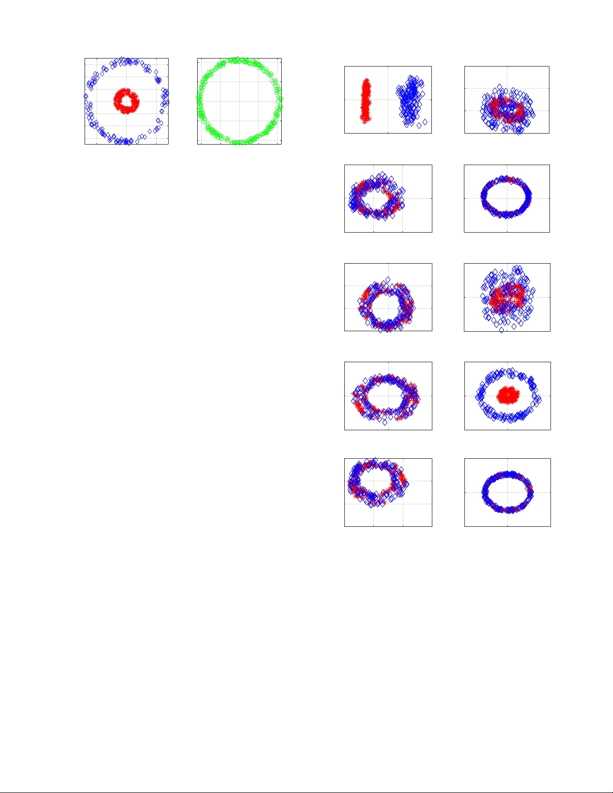
1 Nonlinear Dimensionality Reduction for Discriminati v e Analytics of Multiple Datasets Jia Chen, Gang W ang, Member , IEEE , and Georgios B. Giannakis, F ellow , IEEE Abstract —Principal component analysis (PCA) is widely used for feature extraction and dimensionality reduction, with docu- mented merits in div erse tasks in volving high-dimensional data. PCA copes with one dataset at a time, but it is challenged when it comes to analyzing multiple datasets jointly . In certain data science settings ho wev er , one is often interested in extracting the most discriminative information fr om one dataset of particular interest (a.k.a. target data) r elative to the other(s) (a.k.a. back- ground data). T o this end, this paper puts forth a novel approach, termed discriminative (d) PCA, for such discriminative analytics of multiple datasets. Under certain conditions, dPCA is proved to be least-squares optimal in recov ering the latent subspace vector unique to the target data relativ e to background data. T o account for nonlinear data correlations, (linear) dPCA models for one or multiple background datasets ar e generalized through kernel- based learning. Interestingly , all dPCA variants admit an ana- lytical solution obtainable with a single (generalized) eigenv alue decomposition. Finally , substantial dimensionality reduction tests using synthetic and real datasets are provided to corroborate the merits of the proposed methods. Index T erms —Principal component analysis, discriminative analytics, multiple background datasets, kernel learning. I . I N T R O D U C T I O N Principal component analysis (PCA) is the “workhorse” method for dimensionality reduction and feature extraction. It finds well-documented applications, including statistics, bioin- formatics, genomics, quantitativ e finance, and engineering, to name just a few . The goal of PCA is to obtain low-dimensional representations for high-dimensional data, while preserving most of the high-dimensional data v ariance [22]. Y et, various practical scenarios inv olve multiple datasets, in which one is tasked with extracting the most discriminative in- formation of one target dataset relativ e to others. For instance, consider two gene-expression measurement datasets of volun- teers from across different geographical areas and genders: the first dataset collects gene-expression lev els of cancer patients, considered here as the tar get data , while the second contains lev els from healthy individuals corresponding here to our backgr ound data . The goal is to identify molecular subtypes of cancer within cancer patients. Performing PCA on either the target data or the target together with background data is likely to yield principal components (PCs) that correspond to This work was supported in part by NSF grants 1711471, 1514056, and the NIH grant 1R01GM104975-01. This paper was presented in part at the 43rd IEEE Intl. Conf. on Acoustics, Speech, and Signal Processing, Calgary , Canada, April 15-20, 2018 [36], and the 52nd Asilomar Conf. on Signals, Systems, and Computers, Pacific Grove, CA, October 28-31, 2018 [8]. The authors are with the Digital T echnology Center and the Department of Electrical and Computer Engineering, University of Minnesota, Minneapolis, MN 55455 USA (e-mail: chen5625@umn.edu, gangw ang@umn.edu, geor- gios@umn.edu). the background information common to both datasets (e.g., the demographic patterns and genders) [14], rather than the PCs uniquely describing the subtypes of cancer . Albeit simple to comprehend and practically rele v ant, such discriminativ e data analytics has not been thoroughly addressed. Generalizations of PCA include kernel (K) PCA [30], [33], graph PCA [15], ` 1 -PCA [35], robust PCA [31], multi- dimensional scaling [24], locally linear embedding [28], Isomap [34], and Laplacian eigenmaps [7]. Linear discriminant analysis (LD A) is a supervised classifier of linearly projected reduced dimensionality data vectors. It is designed so that linearly projected training vectors (meaning labeled data) of the same class stay as close as possible, while projected data of different classes are positioned as far as possible [12]. Other discriminativ e methods include re-constructiv e and discrim- inativ e subspaces [11], discriminative vanishing component analysis [20], and k ernel LD A [26], which similar to LD A rely on labeled data. Supervised PCA looks for orthogonal projection vectors so that the dependence of projected vectors from one dataset on the other dataset is maximized [6]. Multiple-factor analysis, an extension of PCA to deal with multiple datasets, is implemented in two steps: S1) normalize each dataset by the largest eigen value of its sample covariance matrix; and, S2) perform PCA on the combined dataset of all normalized ones [1]. On the other hand, canonical correlation analysis is widely employed for analyzing multiple datasets [19], [10], [9], but its goal is to extract the shared low- dimensional structure. The recent proposal called contrasti ve (c) PCA aims at extracting contrastive information between two datasets [2], by searching for directions along which the target data variance is large while that of the background data is small. Carried out using the singular value decomposition (SVD), cPCA can rev eal dataset-specific information often missed by standard PCA if the in volved hyper-parameter is properly selected. Though possible to automatically choose the best hyper-parameter from a list of candidate v alues, perform- ing SVD multiple times can be computationally cumbersome in large-scale feature extraction settings. Building on but going beyond cPCA, this paper starts by dev eloping a no vel approach, termed discriminative (d) PCA, for discriminati ve analytics of two datasets. dPCA looks for linear projections (as in LD A) b ut of unlabeled data vectors, by maximizing the variance of projected target data while minimizing that of background data. This leads to a ratio trace maximization formulation, and also justifies our chosen term discriminative PCA . Under certain conditions, dPCA is proved to be least-squares (LS) optimal in the sense that it reveals PCs specific to the tar get data relati ve to background data. Dif ferent 2 from cPCA, dPCA is parameter free, and it requires a single generalized eigendecomposition, lending itself favorably to large-scale discriminative data analytics. Ho we ver , real data vectors often exhibit nonlinear correlations, rendering dPCA inadequate for complex practical setups. T o this end, nonlinear dPCA is developed via kernel-based learning. Similarly , the solution of KdPCA can be provided analytically in terms of generalized eigen value decompositions. As the complexity of KdPCA gro ws only linearly with the dimensionality of data vectors, KdPCA is preferable ov er dPCA for discriminative analytics of high-dimensional data. dPCA is further extended to handle multiple (more than two) background datasets. Multi-background (M) dPCA is dev eloped to extract low-dimensional discriminativ e structure unique to the target data but not to multiple sets of background data. This becomes possible by maximizing the v ariance of projected target data while minimizing the sum of v ariances of all projected background data. At last, kernel (K) MdPCA is put forth to account for nonlinear data correlations. Notation : Bold uppercase (lo wercase) letters denote matri- ces (column vectors). Operators ( · ) > , ( · ) − 1 , and T r( · ) denote matrix transposition, in verse, and trace, respectiv ely; k a k 2 is the ` 2 -norm of vector a ; diag( { a i } m i =1 ) is a diagonal matrix holding elements { a i } m i =1 on its main diagonal; 0 denotes all- zero vectors or matrices; and I represents identity matrices of suitable dimensions. I I . P R E L I M I N A R I E S A N D P R I O R A RT Consider two datasets, namely a tar get dataset { x i ∈ R D } m i =1 that we are interested in analyzing, and a background dataset { y j ∈ R D } n j =1 that contains latent background-related vectors also present in the target data. Generalization to multi- ple background datasets will be presented in Sec. VI. Assume without loss of generality that both datasets are centered; in other words, the sample mean m − 1 P m i =1 x i ( n − 1 P n j =1 y j ) has been subtracted from each x i ( y j ) . T o motiv ate our novel approaches in subsequent sections, some basics of PCA and cPCA are outlined next. Standard PCA handles a single dataset at a time. It looks for low-dimensional representations { χ i ∈ R d } m i =1 of { x i } m i =1 with d < D as linear projections of { x i } m i =1 by maximizing the variances of { χ i } m i =1 [22]. Specifically for d = 1 , (linear) PCA yields χ i := ˆ u > x i , with the vector ˆ u ∈ R D found by ˆ u := arg max u ∈ R D u > C xx u s . to u > u = 1 (1) where C xx := (1 /m ) P m i =1 x i x > i ∈ R D × D is the sample cov ariance matrix of { x i } m i =1 . Solving (1) yields ˆ u as the normalized eigenv ector of C xx corresponding to the largest eigen value. The resulting projections { χ i = ˆ u > x i } m i =1 con- stitute the first principal component (PC) of the tar get data vectors. When d > 1 , PCA looks for { u i ∈ R D } d i =1 , obtained from the d eigen vectors of C xx associated with the first d largest eigen values sorted in a decreasing order. As alluded to in Sec. I, PCA applied on { x i } m i =1 only , or on the combined datasets {{ x i } m i =1 , { y j } n j =1 } can generally not uncover the discriminativ e patterns or features of the target data relative to the background data. On the other hand, the recent cPCA seeks a vector u ∈ R D along which the target data exhibit large variations while the background data exhibit small variations, via solving [2] max u ∈ R D u > C xx u − α u > C y y u (2a) s . to u > u = 1 (2b) where C y y := (1 /n ) P n j =1 y j y > j ∈ R D × D denotes the sample co variance matrix of { y j } n j =1 , and the hyper -parameter α ≥ 0 trades off maximizing the target data variance (the first term in (2a)) for minimizing the background data variance (the second term). For a giv en α , the solution of (2) is giv en by the eigenv ector of C xx − α C y y associated with its largest eigen v alue, along which the obtained data projections constitute the first contrastiv e (c) PC. Nonetheless, there is no rule of thumb for choosing α . A spectral-clustering based algorithm was devised to automatically select α from a list of candidate values [2], but its brute-force search is computation- ally expensi ve to use in large-scale datasets. I I I . D I S C R I M I NAT I V E P R I N C I PA L C O M P O N E N T A NA L Y S I S Unlike PCA, LDA is a supervised classification method of linearly projected data at reduced dimensionality . It finds those linear projections that reduce that variation in the same class and increase the separation between classes [12]. This is accomplished by maximizing the ratio of the labeled data variance between classes to that within the classes. In a related but unsupervised setup, consider we are giv en a target dataset and a background dataset, and we are tasked with extracting vectors that are meaningful in representing { x i } m i =1 , but not { y j } n j =1 . A meaningful approach would then be to maximize the ratio of the projected target data variance ov er that of the background data. Our discriminative (d) PCA approach finds ˆ u := arg max u ∈ R D u > C xx u u > C y y u (3) W e will term the solution in (3) discriminant subspace vector , and the projections { ˆ u > x i } i =1 the first discriminativ e (d) PC. Next, we discuss the solution in (3). Using Lagrangian duality theory , the solution in (3) corre- sponds to the right eigen vector of C − 1 y y C xx associated with the largest eigen value. T o establish this, note that (3) can be equiv alently rewritten as ˆ u := arg max u ∈ R D u > C xx u (4a) s . to u > C y y u = 1 . (4b) Letting λ denote the dual v ariable associated with the con- straint (4b), the Lagrangian of (4) becomes L ( u ; λ ) = u > C xx u + λ  1 − u > C y y u  . (5) At the optimum ( ˆ u ; ˆ λ ) , the KKT conditions confirm that C xx ˆ u = ˆ λ C y y ˆ u . (6) This is a generalized eigen-equation, whose solution ˆ u is the generalized eigen vector of ( C xx , C y y ) corresponding to 3 the generalized eigenv alue ˆ λ . Left-multiplying (6) by ˆ u > yields ˆ u > C xx ˆ u = ˆ λ ˆ u > C y y ˆ u , corroborating that the optimal objectiv e value of (4a) is attained when ˆ λ := λ 1 is the largest generalized eigen v alue. Furthermore, (6) can be solved efficiently using well-documented solvers that rely on e.g., Cholesky’ s factorization [29]. Supposing further that C y y is nonsingular (6) yields C − 1 y y C xx ˆ u = ˆ λ ˆ u (7) implying that ˆ u in (4) is the right eigenv ector of C − 1 y y C xx corresponding to the largest eigen v alue ˆ λ = λ 1 . T o find multiple ( d ≥ 2 ) subspace vectors, namely { u i ∈ R D } d i =1 that form U := [ u 1 · · · u d ] ∈ R D × d , in (3) with C y y being nonsingular , can be generalized as follows (cf. (3)) ˆ U := arg max U ∈ R D × d T r h  U > C y y U  − 1 U > C xx U i . (8) Clearly , (8) is a ratio trace maximization problem; see e.g., [21], whose solution is giv en in Thm. 1 (see a proof in [13, p. 448]). Theorem 1. Given center ed data { x i ∈ R D } m i =1 and { y j ∈ R D } n j =1 with sample covariance matrices C xx := (1 /m ) P m i =1 x i x > i and C y y := (1 /n ) P n j =1 y j y > j  0 , the i -th column of the dPCA optimal solution ˆ U ∈ R D × d in (8) is given by the right eigen vector of C − 1 y y C xx associated with the i -th larg est eigen value, wher e i = 1 , . . . , d . Our dPCA for discriminati ve analytics of two datasets is summarized in Alg. 1. Four remarks are no w in order . Remark 1 . W ithout background data, we have C y y = I , and dPCA boils down to the standard PCA. Remark 2 . Several possible combinations of tar get and back- ground datasets include: i) measurements from a healthy group { y j } and a diseased group { x i } , where the former has similar population-lev el variation with the latter , but distinct variation due to subtypes of diseases; ii) before-treatment { y j } and after-treatment { x i } datasets, in which the former contains additiv e measurement noise rather than the v ariation caused by treatment; and iii) signal-free { y j } and signal recordings { x i } , where the former consists of only noise. Remark 3 . Consider the eigen v alue decomposition C y y = U y Σ y y U > y . W ith C 1 / 2 y y := Σ 1 / 2 y y U > y , and the definition v := C > / 2 y y u ∈ R D , (4) can be expressed as ˆ v := arg max v ∈ R D v > C − 1 / 2 y y C xx C −> / 2 y y v (9a) s . to v > v = 1 (9b) where ˆ v corresponds to the leading eigenv ector of C − 1 / 2 y y C xx C −> / 2 y y . Subsequently , ˆ u in (4) is recovered as ˆ u = C −> / 2 y y ˆ v . This indeed suggests that discriminativ e analytics of { x i } m i =1 and { y j } n j =1 using dPCA can be viewed as PCA of the ‘denoised’ or ‘background-removed’ data { C − 1 / 2 y y x i } , followed by an ‘in verse’ transformation to map the obtained subspace vector of the { C − 1 / 2 y y x i } data to { x i } that of the target data. In this sense, { C − 1 / 2 y y x i } can be seen as the data Algorithm 1 Discriminative PCA. 1: Input: Nonzero-mean target and background data { ◦ x i } m i =1 and { ◦ y j } n j =1 ; number of dPCs d . 2: Exclude the means from { ◦ x i } and { ◦ y j } to obtain centered data { x i } , and { y j } . Construct C xx and C y y . 3: Perf orm eigendecomposition on C − 1 y y C xx to obtain the d right eigen vectors { ˆ u i } d i =1 associated with the d lar gest eigen values. 4: Output ˆ U = [ ˆ u 1 · · · ˆ u d ] . obtained after removing the dominant ‘background’ subspace vectors from the target data. Remark 4 . Inexpensi ve po wer or Lanczos iterations [29] can be employed to compute the principal eigen vectors in (7). Consider again (4). Based on Lagrange duality , when se- lecting α = ˆ λ in (2), where ˆ λ is the lar gest eigenv alue of C − 1 y y C xx , cPCA maximizing u > ( C xx − ˆ λ C y y ) u is equiv alent to max u ∈ R D L ( u ; ˆ λ ) = u > ( C xx − ˆ λ C y y ) u + ˆ λ , which coin- cides with (5) when λ = ˆ λ at the optimum. This suggests that the optimizers of cPCA and dPCA share the same direction when α in cPCA is chosen to be the optimal dual variable ˆ λ of our dPCA in (4). This equiv alence between dPCA and cPCA with a proper α can also be seen from the follo wing. Theorem 2. [16, Theor em 2] F or real symmetric matrices C xx  0 and C y y  0 , the following holds ˇ λ = ˇ u > C xx ˇ u ˇ u > C y y ˇ u = max k u k 2 =1 u > C xx u u > C y y u if and only if ˇ u > ( C xx − ˇ λ C y y ) ˇ u = max k u k 2 =1 u > ( C xx − ˇ λ C y y ) u . T o gain further insight into the relationship between dPCA and cPCA, suppose that C xx and C y y are simultaneously di- agonalizable; that is, there exists an unitary matrix U ∈ R D × D such that C xx := UΣ xx U > , and C y y := UΣ y y U > where diagonal matrices Σ xx , Σ y y  0 hold accordingly eigen values { λ i x } D i =1 of C xx and { λ i y } D i =1 of C y y on their main diagonals. Even if the two datasets may share some subspace vectors, { λ i x } D i =1 and { λ i y } D i =1 are in general not the same. It is easy to check that C − 1 y y C xx = UΣ − 1 y y Σ xx U > = U diag  { λ i x λ i y } D i =1  U > . Seeking the first d latent subspace vectors is tantamount to taking the d columns of U that correspond to the d largest values among { λ i x λ i y } D i =1 . On the other hand, cPCA for a fixed α , looks for the first d latent subspace vectors of C xx − α C y y = U ( Σ xx − α Σ y y ) U > = U diag  { λ i x − αλ i y } D i =1  U > , which amounts to taking the d columns of U associated with the d largest values in { λ i x − αλ i y } D i =1 . This further confirms that when α is suf- ficiently large (small), cPCA returns the d columns of U associated with the d largest λ i y ’ s ( λ i x ’ s). When α is not properly chosen, cPCA may fail to extract the most contrastive information from target data relati ve to background data. In 4 contrast, this is not an issue is not present in dPCA simply because it has no tunable parameter . I V . O P T I M A L I T Y O F D P C A In this section, we show that dPCA is optimal when data obey a certain af fine model. In a similar vein, PCA adopts a factor analysis model to express the non-centered background data { ◦ y j ∈ R D } n j =1 as ◦ y j = m y + U b ψ j + e y ,j , j = 1 , . . . , n (10) where m y ∈ R D denotes the unkno wn location (mean) vector; U b ∈ R D × k has orthonormal columns with k < D ; { ψ j ∈ R k } n j =1 are some unkno wn coefficients with co v ariance matrix Σ b := diag ( λ y , 1 , λ y , 2 , . . . , λ y ,k ) ∈ R k × k ; and the modeling errors { e y ,j ∈ R D } n j =1 are assumed zero-mean with cov ariance matrix E [ e y ,j e > y ,j ] = I . Adopting the least- squares (LS) criterion, the unkno wns m y , U b , and { ψ j } can be estimated by [37] min m y , { ψ j } U b n X j =1 k ◦ y j − m y − U b ψ j k 2 2 s . to U > b U b = I we find at the optimum ˆ m y := (1 /n ) P n j =1 ◦ y j ,  ˆ ψ j := ˆ U > b ( ◦ y j − ˆ m y )  , with ˆ U b columns giv en by the first k leading eigen vectors of C y y = (1 /n ) P n j =1 y j y > j , in which y j := ◦ y j − ˆ m y . It is clear that E [ y j y > j ] = U b Σ b U > b + I . Let matrix U n ∈ R D × ( D − k ) with orthonormal columns satisfying U > n U b = 0 , and U y := [ U b U n ] ∈ R D × D with Σ y := diag( { λ y ,i } D i =1 ) , where { λ y ,k + ` := 1 } D − k ` =1 . Therefore, U b Σ b U > b + I = U y Σ y U > y . As n → ∞ , the strong law of large numbers asserts that C y y → E [ y j y > j ] ; that is, C y y = U y Σ y U > y as n → ∞ . Here we assume that the target data { ◦ x i ∈ R D } m i =1 share the background related matrix U b with data { ◦ y j } , b ut also hav e d extra vectors specific to the target data relativ e to the background data. This assumption is well justified in realistic setups. In the example discussed in Sec. I, both patients’ and healthy persons’ gene-expression data contain common patterns corresponding to geographical and gender variances; while the patients’ gene-expression data contain some specific latent subspace vectors corresponding to their diseases. Focusing for simplicity on d = 1 , we model { ◦ x i } as ◦ x i = m x + [ U b u s ]  χ b,i χ s,i  + e x,i , i = 1 , . . . , m (11) where m x ∈ R D represents the location of { ◦ x i } m i =1 ; { e x,i } m i =1 account for zero-mean modeling errors; U x := [ U b u s ] ∈ R D × ( k +1) collects orthonormal columns, where U b is the shared latent subspace vectors associated with background data, and u s ∈ R D is a latent subspace vector unique to the target data, but not to the background data. Simply put, our goal is to extract this discriminative subspace u s giv en { ◦ x i } m i =1 and { ◦ y j } n j =1 . Similarly , giv en { ◦ x i } , the unkno wns m x , U x , and { χ i := [ χ > b,i , χ s,i ] > } can be estimated by max m x , { χ i } U x m X i =1 k ◦ x i − m x − U x χ i k 2 2 s . to U > x U x = I yielding ˆ m x := (1 /m ) P m i =1 ◦ x i , ˆ χ i := ˆ U > x x i with x i := ◦ x i − ˆ m x , where ˆ U x has columns the ( k + 1) principal eigen vectors of C xx = (1 /m ) P m i =1 x i x > i . When m → ∞ , it holds that C xx = U x Σ x U > x , with Σ x := E [ χ i χ > i ] = diag( λ x, 1 , λ x, 2 , . . . , λ x,k +1 ) ∈ R ( k +1) × ( k +1) . Let Σ x,k ∈ R k × k denote the submatrix of Σ x formed by its first k rows and columns. When m, n → ∞ and C y y is nonsingular , one can e xpress C − 1 y y C xx as U y Σ − 1 y U > y U x Σ x U > x = [ U b U n ]  Σ − 1 b 0 0 I   I 0 0 U > n u s  ×  Σ x,k 0 0 λ x,k +1   U > b u > s  = [ U b U n ]  Σ − 1 b Σ x,k 0 0 λ x,k +1 U > n u s   U > b u > s  = U b Σ − 1 b Σ x,k U > b + λ x,k +1 U n U > n u s u > s . Observe that the first and second summands ha ve rank k and 1 , respecti vely , implying that C − 1 y y C xx has at most rank k + 1 . If u b,i denotes the i -th column of U b , that is orthogonal to { u b,j } k j =1 ,j 6 = i and u s , right-multiplying C − 1 y y C xx by u b,i yields C − 1 y y C xx u b,i = ( λ x,i /λ y ,i ) u b,i for i = 1 , . . . , k , which hints that { u b,i } k i =1 are k eigen vec- tors of C − 1 y y C xx associated with eigen v alues { λ x,i /λ y ,i } k i =1 . Again, right-multiplying C − 1 y y C xx by u s giv es rise to C − 1 y y C xx u s = λ x,k +1 U n U > n u s u > s u s = λ x,k +1 U n U > n u s . (12) T o proceed, we will leverage the following three facts: i) u s is orthogonal to all columns of U b ; ii) columns of U n are orthogonal to those of U b ; and iii) [ U b U n ] has full rank. Based on i)-iii), it follo ws readily that u s can be uniquely expressed as a linear combination of columns of U n ; that is, u s := P D − k i =1 p i u n,i , where { p i } D − k i =1 are some unknown coefficients, and u n,i denotes the i -th column of U n . One can manipulate U n U > n u s in (12) as U n U > n u s = [ u n, 1 · · · u n,D − k ]    u > n, 1 u s . . . u > n,D − k u s    = u n, 1 u > n, 1 u s + · · · + u n,D − k u > n,D − k u s = p 1 u n, 1 + · · · + p D − k u n,D − k = u s yielding C − 1 y y C xx u s = λ x,k +1 u s ; that is, u s is the ( k + 1) -st eigen vector of C − 1 y y C xx corresponding to eigen v alue λ x,k +1 . Before moving on, we will make two assumptions. Assumption 1. Backgr ound and tar get data ar e generated accor ding to the models (10) and (11) , r espectively , with the backgr ound data sample covariance matrix being nonsingular . Assumption 2. It holds for all i = 1 , . . . , k that λ x,k +1 /λ y ,k +1 > λ x,i /λ y ,i . Assumption 2 essentially requires that u s is discriminativ e enough in the target data relativ e to the background data. After 5 combining Assumption 2 and the fact that u s is an eigenv ector of C − 1 y y C xx , it follows readily that the eigen vector of C − 1 y y C xx associated with the largest eigen v alue is u s . Under these two assumptions, we establish the optimality of dPCA next. Theorem 3. Under Assumptions 1 and 2 with d = 1 , as m, n → ∞ , the solution of (3) r ecovers the subspace vector specific to tar get data relative to backgr ound data, namely u s . V . K E R N E L D P C A W ith advances in data acquisition and data storage technolo- gies, a sheer v olume of possibly high-dimensional data are collected daily , that topologically lie on a nonlinear manifold in general. This goes beyond the ability of the (linear) dPCA in Sec. III due mainly to a couple of reasons: i) dPCA presumes a linear low-dimensional hyperplane to project the target data vectors; and ii) dPCA incurs computational com- plexity O (max( m, n ) D 2 ) that gro ws quadratically with the dimensionality of data vectors. T o address these challenges, this section generalizes dPCA to account for nonlinear data relationships via kernel-based learning, and puts forth kernel (K) dPCA for nonlinear discriminativ e analytics. Specifically , KdPCA starts by mapping both the target and background data vectors from the original data space to a higher-dimensional (possibly infinite-dimensional) feature space using a common nonlinear function, which is followed by performing linear dPCA on the transformed data. Consider first the dual version of dPCA, starting with the N := m + n augmented data { z i ∈ R D } N i =1 as z i :=  x i , 1 ≤ i ≤ m y i − m , m < i ≤ N and e xpress the wanted subspace vector u ∈ R D in terms of Z := [ z 1 · · · z N ] ∈ R D × N , yielding u := Za , where a ∈ R N denotes the dual vector . When min( m , n )  D , matrix Z has full ro w rank in general. Thus, there always exists a vector a so that u = Za . Similar steps have also been used in obtaining dual versions of PCA and CCA [30], [32]. Substituting u = Za into (3) leads to our dual dPCA max a ∈ R N a > Z > C xx Za a > Z > C y y Za (13) based on which we will de velop our KdPCA in the sequel. Similar to deriving KPCA from dual PCA [30], our ap- proach is first to transform { z i } N i =1 from R D to a high- dimensional space R L (possibly with L = ∞ ) by some nonlinear mapping function φ ( · ) , followed by removing the sample means of { φ ( x i ) } and { φ ( y j ) } from the corre- sponding transformed data; and subsequently , implementing dPCA on the centered transformed datasets to obtain the lo w- dimensional kernel dPCs. Specifically , the sample cov ariance matrices of { φ ( x i ) } m i =1 and { φ ( y j ) } n j =1 can be expressed as C φ xx := 1 m m X i =1 ( φ ( x i ) − µ x ) ( φ ( x i ) − µ x ) > ∈ R L × L C φ y y := 1 n n X j =1 ( φ ( y j ) − µ y ) ( φ ( y j ) − µ y ) > ∈ R L × L Algorithm 2 Kernel dPCA. 1: Input: T arget data { x i } m i =1 and background data { y j } n j =1 ; number of dPCs d ; kernel function κ ( · ) ; constant  . 2: Construct K using (15). Build K x and K y via (16). 3: Solve (19) to obtain the first d eigen vectors { ˆ a i } d i =1 . 4: Output ˆ A := [ ˆ a 1 · · · ˆ a d ] . where the L -dimensional vectors µ x := (1 /m ) P m i =1 φ ( x i ) and µ y := (1 /n ) P n j =1 φ ( y j ) are accordingly the sample means of { φ ( x i ) } and { φ ( y j ) } . For con venience, let Φ ( Z ) := [ φ ( x 1 ) − µ x , · · · , φ ( x m ) − µ x , φ ( y 1 ) − µ y , · · · , φ ( y n ) − µ y ] ∈ R L × N . Upon replacing { x i } and { y j } in (13) with { φ ( x i ) − µ x } and { φ ( y j ) − µ y } , respectiv ely , the kernel version of (13) boils down to max a ∈ R N a > Φ > ( Z ) C φ xx Φ ( Z ) a a > Φ > ( Z ) C φ y y Φ ( Z ) a . (14) In the sequel, (14) will be further simplified by lev eraging the so-termed ‘kernel trick’ [3]. T o start, define a kernel matrix K xx ∈ R m × m of { x i } whose ( i, j ) -th entry is κ ( x i , x j ) := h φ ( x i ) , φ ( x j ) i for i, j = 1 , . . . , m , where κ ( · ) represents some kernel function. Matrix K y y ∈ R n × n of { y j } is defined likewise. Further , the ( i, j ) -th entry of matrix K xy ∈ R m × n is κ ( x i , y j ) := h φ ( x i ) , φ ( y j ) i . Centering K xx , K y y , and K xy produces K c xx := K xx − 1 m 1 m K xx − 1 m K xx 1 m + 1 m 2 1 m K xx 1 m K c y y := K y y − 1 n 1 n K y y − 1 n K y y 1 n + 1 n 2 1 n K y y 1 n K c xy := K xy − 1 m 1 m K xy − 1 n K xy 1 n + 1 mn 1 m K xy 1 n with matrices 1 m ∈ R m × m and 1 n ∈ R n × n having all entries 1 . Based on those centered matrices, let K :=  K c xx K c xy ( K c xy ) > K c y y  ∈ R N × N . (15) Define further K x ∈ R N × N and K y ∈ R N × N with ( i, j ) -th entries K x i,j :=  K i,j /m 1 ≤ i ≤ m 0 m < i ≤ N (16a) K y i,j :=  0 1 ≤ i ≤ m K i,j /n m < i ≤ N (16b) where K i, j stands for the ( i, j ) -th entry of K . Using (15) and (16), it can be easily verified that KK x = K diag( { ι x i } N i =1 ) K , and KK y = K diag( { ι y i } N i =1 ) K , where { ι x i = 1 } m i =1 , { ι x i = 0 } N i = m +1 , { ι y i = 0 } m i =1 , and { ι y i = 1 } N i = m +1 . That is, both KK x and KK y are symmetric. Substituting (15) and (16) into (14) yields (see details in the Appendix) max a ∈ R N a > KK x a a > KK y a . (17) Due to the rank-deficiency of KK y howe ver , (17) does not admit a meaningful solution. T o address this issue, follo wing kPCA [30], [32], a positiv e constant  > 0 is added to the 6 diagonal entries of KK y . Hence, our KdPCA formulation for d = 1 is gi ven by ˆ a := arg max a ∈ R N a > KK x a a > ( KK y +  I ) a . (18) Along the lines of dPCA, the solution of KdPCA in (18) can be provided by ( KK y +  I ) − 1 KK x ˆ a = ˆ λ ˆ a . (19) The optimizer ˆ a coincides with the right eigenv ector of ( KK y +  I ) − 1 KK x corresponding to the largest eigen value ˆ λ = λ 1 . When looking for d dPCs, with { a i } d i =1 collected as columns in A := [ a 1 · · · a d ] ∈ R N × d , the KdPCA in (18) can be generalized to d ≥ 2 as ˆ A := arg max A ∈ R N × d T r  A > ( KK y +  I  A ) − 1 A > KK x A  whose columns correspond to the d right eigen vectors of ( KK y +  I ) − 1 KK x associated with the d lar gest eigen val- ues. Having found ˆ A , one can project the data Φ ( Z ) onto the obtained d subspace vectors by K ˆ A . It is worth remarking that KdPCA can be performed in the high-dimensional feature space without explicitly forming and e v aluating the nonlinear transformations. Indeed, this becomes possible by the ‘kernel trick’ [3]. The main steps of KdPCA are giv en in Alg. 2. T wo remarks are worth making at this point. Remark 5 . When the kernel function required to form K xx , K y y , and K xy is not given, one may use the multi-kernel learning method to automatically choose the right kernel function(s); see for example, [4], [38], [39]. Specifically , one can presume K xx := P P i =1 δ i K i xx , K y y := P P i =1 δ i K i y y , and K xy := P P i =1 δ i K i xy in (18), where K i xx ∈ R m × m , K i y y ∈ R n × n , and K i xy ∈ R m × n are formed using the kernel function κ i ( · ) ; and { κ i ( · ) } P i =1 are a preselected dictionary of known kernels, but { δ i } P i =1 will be treated as unknowns to be learned along with A in (18). Remark 6 . In the absence of background data, upon setting { φ ( y j ) = 0 } , and  = 1 in (18), matrix ( KK y +  I ) − 1 KK x reduces to M :=  ( K c xx ) 2 0 0 0  . After collecting the first m entries of ˆ a i into w i ∈ R m , (19) suggests that ( K c xx ) 2 w i = λ i w i , where λ i denotes the i -th largest eigen v alue of M . Clearly , { w i } d i =1 can be viewed as the d eigen vectors of ( K c xx ) 2 associated with their d largest eigen values. Recall that KPCA finds the first d principal eigen vectors of K c xx [30]. Thus, KPCA is a special case of KdPCA, when no background data are employed. V I . D I S C R I M I NA T I V E A N A L Y T I C S W I T H M U LT I P L E B AC K G R O U N D D AT A S E T S So far , we have presented discriminativ e analytics methods for two datasets. This section presents their generalizations to cope with multiple (specifically , one target plus more than one background) datasets. Suppose that, in addition to the zero- mean target dataset { x i ∈ R D } m i =1 , we are also giv en M ≥ 2 Algorithm 3 Multi-background dPCA. 1: Input: T arget data { ◦ x i } m i =1 and background data { ◦ y k j } n k j =1 for k = 1 , . . . , M ; weight hyper-parameters { ω k } M k =1 ; number of dPCs d . 2: Remove the means from { ◦ x i } and { ◦ y k j } M k =1 to obtain { x i } and { y k j } M k =1 . Form C xx , { C k y y } M k =1 , and C y y := P M k =1 ω k C k y y . 3: Perf orm eigendecomposition on C − 1 y y C xx to obtain the first d right eigenv ectors { ˆ u i } d i =1 . 4: Output ˆ U := [ ˆ u 1 · · · ˆ u d ] . centered background datasets { y k j } n k j =1 for k = 1 , . . . , M . The M sets of background data { y k j } M k =1 contain latent background subspace vectors that are also present in { x i } . Let C xx := m − 1 P m i =1 x i x > i and C k y y := n − 1 k × P n k j =1 y k j ( y k j ) > be the corresponding sample cov ariance matri- ces. The goal here is to un veil the latent subspace vectors that are significant in representing the target data, but not any of the background data. Building on the dPCA in (8) for a single background dataset, it is meaningful to seek directions that maximize the variance of target data, while minimizing those of all background data. Formally , we pursue the following optimization, that we term multi-background (M) dPCA here, for discriminativ e analytics of multiple datasets max U ∈ R D × d T r  M X k =1 ω k U > C k y y U  − 1 U > C xx U  (20) where { ω k ≥ 0 } M k =1 with P M k =1 ω k = 1 weight the v ariances of the M projected background datasets. Upon defining C y y := P M k =1 ω k C k y y , it is straightforward to see that (20) reduces to (8). Therefore, one readily deduces that the optimal U in (20) can be obtained by taking the d right eigen vectors of C − 1 y y C xx that are associated with the d largest eigen v alues. For implementation, the steps of MdPCA are presented in Alg. 3. Remark 7 . The parameters { ω k } M k =1 can be decided using two possible methods: i) spectral-clustering [27] to select a few sets of { ω k } yielding the most representative subspaces for projecting the target data across { ω k } ; or ii) optimizing { ω k } M k =1 jointly with U in (20). For data belonging to nonlinear manifolds, kernel (K) MdPCA will be developed next. W ith some nonlinear function φ ( · ) , we obtain the transformed target data { φ ( x i ) ∈ R L } as well as background data { φ ( y k j ) ∈ R L } . Letting µ x ∈ R L and µ k y := (1 /n k ) P n k j =1 φ ( y k j ) ∈ R L denote the means of { φ ( x i ) } and { φ ( y k j ) } , respectiv ely , one can form the corresponding cov ariance matrices C φ xx ∈ R L × L , and C φ,k y y := 1 n k n k X j =1  φ ( y k j ) − µ k y   φ ( y k j ) − µ k y  > ∈ R L × L 7 for k = 1 , . . . , M . Define the aggregate vector b i ∈ R L b i :=          φ ( x i ) − µ x , 1 ≤ i ≤ m φ ( y 1 i − m ) − µ 1 y , m < i ≤ m + n 1 . . . φ ( y M i − ( N − n M ) ) − µ M y , N − n M < i ≤ N where N := m + P M k =1 n k , for i = 1 , . . . , N , and collect vectors { b i } N i =1 as columns to form B := [ b 1 · · · b N ] ∈ R L × N . Upon assembling dual vectors { a i ∈ R N } d i =1 to form A := [ a 1 · · · a d ] ∈ R N × d , the kernel version of (20) can be obtained as max A ∈ R N × d T r  A > B > M X k =1 ω k C φ,k y y BA  − 1 A > B > C φ xx BA  . Consider no w kernel matrices K xx ∈ R m × m and K kk ∈ R n k × n k , whose ( i, j ) -th entries are κ ( x i , x j ) and κ ( y k i , y k j ) , respectiv ely , for k = 1 , . . . , M . Furthermore, matrices K xk ∈ R m × n k , and K lk ∈ R n l × n k are defined with their cor- responding ( i, j ) -th elements κ ( x i , y k j ) and κ ( y l i , y k j ) , for l = 1 , . . . , k − 1 and k = 1 , . . . , M . W e subsequently center those matrices to obtain K c xx and K c kk := K kk − 1 n k 1 n k K kk − 1 n k K kk 1 n k + 1 n 2 k 1 n k K kk 1 n k K c xk := K xk − 1 m 1 m K xk − 1 n k K xk 1 n k + 1 mn k 1 m K xk 1 n k K c lk := K lk − 1 n l 1 n l K lk − 1 n k K lk 1 n k + 1 n l n k 1 n l K lk 1 n k where 1 n k ∈ R n k × n k and 1 n l ∈ R n l × n l are all-one matrices. W ith K x as in (16a), consider the N × N matrix K :=      K c xx K c x 1 · · · K c xM ( K c x 1 ) > K c 11 · · · K c 1 M . . . . . . . . . . . . ( K c xM ) > ( K c 1 M ) > · · · K c M M      (21) and K k ∈ R N × N with ( i, j ) -th entry K k i,j :=  K i,j /n k , if m + P n k − 1 ` =1 n ` < i ≤ m + P n k ` =1 n ` 0 , otherwise (22) for k = 1 , . . . , M . Adopting the regularization in (18), our KMdPCA finds ˆ A := arg max A ∈ R N × d T r  A >  K M X k =1 K k +  I  A  − 1 A > KK x A  similar to (K)dPCA, whose solution comprises the right eigen- vectors associated with the first d largest eigen values in  K M X k =1 K k +  I  − 1 KK x ˆ a i = ˆ λ i ˆ a i . (23) For implementation, KMdPCA is presented in Alg. 4. Remark 8 . W e can verify that PCA, KPCA, dPCA, KdPCA, MdPCA, and KMdPCA incur computational complexities O ( mD 2 ) , O ( m 2 D ) , O (max( m, n ) D 2 ) , O (max( m 2 , n 2 ) D ) , O (max( m, ¯ n ) D 2 ) , and O (max( m 2 , ¯ n 2 ) D ) , respecti vely , where ¯ n := max k { n k } M k =1 . It is also not dif ficult to check that the computational complexity of forming C xx , C y y , C − 1 y y , and performing the eigendecomposition on C − 1 y y C xx Algorithm 4 Kernel multi-background dPCA. 1: Input: T arget data { x i } m i =1 and background data { y k j } n k j =1 for k = 1 , . . . , M ; number of dPCs d ; kernel function κ ( · ) ; weight coefficients { ω k } M k =1 ; constant  . 2: Construct K using (21). Build K x and { K k } M k =1 via (16a) and (22). 3: Solve (23) to obtain the first d eigen vectors { ˆ a i } d i =1 . 4: Output ˆ A := [ ˆ a 1 · · · ˆ a d ] . is O ( mD 2 ) , O ( nD 2 ) , O ( D 3 ) , and O ( D 3 ) , respecti vely . As the number of data vectors ( m, n ) is much larger than their dimensionality D , when performing dPCA in the pri- mal domain, it follows readily that dPCA incurs complex- ity O (max( m, n ) D 2 ) . Similarly , the computational com- plexities of the other algorithms can be checked.Evidently , when min( m, n )  D or min( m, n )  D with n := min k { n k } M k =1 , dPCA and MdPCA are computationally more attractiv e than KdPCA and KMdPCA. On the other hand, KdPCA and KMdPCA become more appealing, when D  max( m, n ) or D  max( m, ¯ n ) . Moreover , the computational complexity of cPCA is O (max( m, n ) D 2 L ) , where L denotes the number of α ’ s candidates. Clearly , relativ e to dPCA, cPCA is computationally more expensiv e when DL > max( m, n ) . V I I . N U M E R I C A L T E S T S T o ev aluate the performance of our proposed approaches for discriminativ e analytics, we carried out a number of numerical tests using several synthetic and real-world datasets, a sample of which are reported in this section. A. dPCA tests Semi-synthetic target { ◦ x i ∈ R 784 } 2 , 000 i =1 and background images { ◦ y j ∈ R 784 } 3 , 000 j =1 were obtained by superimposing images from the MNIST 1 and CIF AR-10 [23] datasets. Specifically , the target data { x i ∈ R 784 } 2 , 000 i =1 were generated using 2 , 000 handwritten digits 6 and 9 (1,000 for each) of size 28 × 28 , superimposed with 2 , 000 frog images from the CIF AR-10 database [23] followed by removing the sample mean from each data point; see Fig. 1. The raw 32 × 32 frog images were con verted into grayscale, and randomly cropped to 28 × 28 . The zero-mean background data { y j ∈ R 784 } 3 , 000 j =1 were constructed using 3 , 000 cropped frog images, which were randomly chosen from the remaining frog images in the CIF AR-10 database. The dPCA Alg. 1 was performed on { ◦ x i } and { ◦ y j } with d = 2 . PCA was implemented on { ◦ x i } only . The first two PCs and dPCs are presented in the left and right panels of Fig. 2, respectively . Clearly , dPCA re veals the discriminati ve information of the target data describing digits 6 and 9 relativ e to the background data, enabling successful discovery of the digit 6 and 9 subgroups. On the contrary , PCA captures only the patterns that correspond to the generic background rather than those associated with the digits 6 and 9 . T o further assess the performance of dPCA and PCA, K-means is 1 Downloaded from http://yann.lecun.com/exdb/mnist/. 8 Fig. 1: Superimposed images. -500 0 500 dPC1 0 1000 2000 3000 4000 dPC2 dPCA -3000 -2500 -2000 -1500 -1000 -500 PC1 0 1000 2000 3000 4000 PC2 PCA digit-6 digit-9 Fig. 2: dPCA versus PCA on semi-synthetic images. carried out using the resulting low-dimensional representations of the target data. The clustering performance is ev aluated in terms of two metrics: clustering error and scatter ratio. The clustering error is defined as the ratio of the number of incorrectly clustered data vectors ov er m . Scatter ratio verifying cluster separation is defined as S t / P 2 i =1 S i , where S t and { S i } 2 i =1 denote the total scatter value and the within cluster scatter v alues, gi ven by S t := P 2 , 000 j =1 k ˆ U > x j k 2 2 and { S i := P j ∈C i k ˆ U > x j − ˆ U > P k ∈C i x k k 2 2 } 2 i =1 , respecti vely , with C i representing the set of data vectors belonging to cluster i . T able I reports the clustering errors and scatter ratios of dPCA and PCA under dif ferent d values. Clearly , dPCA exhibits lower clustering error and higher scatter ratio. Real protein expression data [18] were also used to ev aluate the ability of dPCA to discov er subgroups in real-world conditions. T arget data { ◦ x i ∈ R 77 } 267 i =1 contained 267 data vectors, each collecting 77 protein expression measurements of a mouse having Down Syndrome disease [18]. In particular, the first 135 data points { ◦ x i } 135 i =1 recorded protein expression measurements of 135 mice with drug-memantine treatment, while the remaining { ◦ x i } 267 i =136 collected measurements of 134 mice without such treatment. Background data { ◦ y j ∈ R 77 } 135 j =1 on the other hand, comprised such measurements from 135 healthy mice, which likely exhibited similar natural variations (due to e.g., age and sex) as the target mice, but without the differences that result from the Do wn Syndrome disease. When performing cPCA on { ◦ x i } and { ◦ y j } , four α ’ s were selected from 15 logarithmically-spaced values between 10 − 3 and 10 3 via the spectral clustering method presented in [2]. Experimental results are reported in Fig. 3 with red circles and black diamonds representing sick mice with and without treatment, respecti vely . Evidently , when PCA is applied, the low-dimensional representations of the protein measurements from mice with and without treatment are distributed similarly . In contrast, the lo w-dimensional representations cluster two groups of mice successfully when dPCA is employed. At the T ABLE I: Performance comparison between dPCA and PCA. d Clustering error Scatter ratio dPCA PCA dPCA PCA 1 0.1660 0.4900 2.0368 1.0247 2 0.1650 0.4905 1.8233 1.0209 3 0.1660 0.4895 1.6719 1.1327 4 0.1685 0.4885 1.4557 1.1190 5 0.1660 0.4890 1.4182 1.1085 10 0.1680 0.4885 1.2696 1.0865 50 0.1700 0.4880 1.0730 1.0568 100 0.1655 0.4905 1.0411 1.0508 -5 0 5 cPC1 -2 -1 0 1 2 cPC2 cPCA, , = 3.5938 -2 0 2 cPC1 -2 -1 0 1 2 cPC2 cPCA, , = 27.8256 -1 0 1 cPC1 -0.4 -0.2 0 0.2 0.4 0.6 cPC2 cPCA, , = 215.4435 -5 0 5 dPC1 -2 -1 0 1 2 dPC2 dPCA -2 0 2 4 PC1 -5 0 5 PC2 PCA -5 0 5 cPC1 -2 -1 0 1 2 3 cPC2 cPCA, , = 0.001 with treatment without treatment Fig. 3: Discovering subgroups in mice protein expression data. price of runtime (about 15 times more than dPCA), cPCA with well tuned parameters ( α = 3 . 5938 and 27 . 8256 ) can also separate the two groups. B. KdPCA tests In this subsection, our KdPCA is e valuated using syn- thetic and real data. By adopting the procedure de- scribed in [17, p. 546], we generated target data { x i := 9 -5 0 5 x i,1 -6 -4 -2 0 2 4 6 x i,2 -10 -5 0 5 10 x i,3 -10 -5 0 5 10 x i,4 Fig. 4: T arget data dimension distributions with x i,j representing the j -th entry of x i for j = 1 , . . . , 4 and i = 1 , . . . , 300 . [ x i, 1 x i, 2 x i, 3 x i, 4 ] > } 300 i =1 and background data { y j ∈ R 4 } 150 j =1 . In detail, { [ x i, 1 x i, 2 ] > } 300 i =1 were sampled uniformly from two circular concentric clusters with corresponding radii 1 and 6 shown in the left panel of Fig. 4; and { [ x i, 3 x i, 4 ] > } 300 i =1 were uniformly drawn from a circle with radius 10 ; see Fig. 4 (right panel) for illustration. The first and second two dimensions of { y j } 150 j =1 were uniformly sampled from two concentric circles with corresponding radii of 4 and 10 . All data points in { x i } and { y j } were corrupted with additiv e noise sampled independently from N ( 0 , 0 . 1 I ) . T o un veil the specific cluster structure of the tar get data relativ e to the background data, Alg. 2 was run with  = 10 − 3 and using the de gree- 2 polynomial kernel κ ( z i , z j ) = ( z > i z j ) 2 . Competing alternatives including PCA, KPCA, cPCA, kernel (K) cPCA [2], and dPCA were also implemented. Further , KPCA and KcPCA shared the kernel function with KdPCA. Three different values of α were automatically chosen for cPCA [2]. The parameter α of KcPCA was set as 1 , 10 , and 100 . Figure 5 depicts the first two dPCs, cPCs, and PCs of the aforementioned dimensionality reduction algorithms. Clearly , only KdPCA successfully re veals the two unique clusters of { x i } relativ e to { y j } . KdPCA was tested in realistic settings using the real Mobile (M) Health data [5]. This dataset consists of sensor (e.g., gyroscopes, accelerometers, and EKG) measurements from volunteers conducting a series of physical activities. In the first experiment, 200 target data { x i ∈ R 23 } 200 i =1 were used, each of which recorded 23 sensor measurements from one volunteer performing two different physical activities, namely laying do wn and having frontal elev ation of arms ( 100 data points correspond to each activity). Sensor measurements from the same volunteer standing still were utilized for the 100 background data points { y j ∈ R 23 } 100 j =1 . For KdPCA, KPCA, and KcPCA algorithms, the Gaussian kernel with bandwidth 5 was used. Three different values for the parameter α in cPCA were automatically selected from a list of 40 logarithmically- spaced values between 10 − 3 and 10 3 , whereas α in KcPCA was set to 1 [2]. The first two dPCs, cPCs, and PCs of KdPCA, dPCA, KcPCA, cPCA, KPCA, and PCA are reported in Fig. 6. It is self-evident that the two activities ev olve into two separate clusters in the plots of KdPCA and KcPCA. On the contrary , due to the nonlinear data correlations, the other alternativ es fail to distinguish the two activities. -20 0 20 dPC1 -10 0 10 20 dPC2 dPCA -20 0 20 PC1 -20 0 20 PC2 PCA -1 0 1 dPC1 -2 0 2 dPC2 KdPCA -100 0 100 200 PC1 -200 -100 0 100 PC2 KPCA -20 0 20 cPC1 -20 0 20 cPC2 cPCA, , = 0.30392 -20 0 20 cPC1 -10 0 10 cPC2 cPCA, , = 2.0434 -10 0 10 cPC1 -10 0 10 cPC2 cPCA, , = 13.7382 -20 0 20 40 cPC1 -20 0 20 cPC2 KcPCA, , = 1 -200 0 200 cPC1 -100 0 100 200 cPC2 KcPCA, , = 10 -200 0 200 cPC1 -200 0 200 cPC2 KcPCA, , = 100 Fig. 5: Discovering subgroups in nonlinear synthetic data. In the second experiment, the target data were formed with sensor measurements of one v olunteer executing waist bends forward and c ycling. The background data were collected from the same v olunteer standing still. The Gaussian kernel with bandwidth 40 was used for KdPCA and KPCA, while the second-order polynomial kernel κ ( z i , z j ) = ( z > i z j + 3) 2 was employed for KcPCA. The first two dPCs, cPCs, and PCs of simulated schemes are depicted in Fig. 7. Evidently , KdPCA outperforms its competing alternatives in discovering the two physical activities of the tar get data. T o test the scalability of our developed schemes, the Ex- tended Y ale-B (EYB) face image dataset [25] was adopted to test the clustering performance of KdPCA, KcPCA, and 10 -20 0 20 dPC1 -0.5 0 0.5 1 dPC2 KdPCA -1 0 1 PC1 -0.5 0 0.5 1 PC2 KPCA -200 0 200 dPC1 -200 -100 0 100 DdPC2 dPCA -200 0 200 400 PC1 -200 0 200 PC2 PCA -200 0 200 cPC1 -200 0 200 400 cPC2 cPCA, , = 8.5317 lying down elevation of arms -200 0 200 cPC1 -400 -200 0 200 cPC2 cPCA, , = 148.7352 -200 0 200 cPC1 -400 -200 0 200 cPC2 cPCA, , = 621.0169 -100 0 100 cPC1 -1 -0.5 0 0.5 cPC2 KcPCA Fig. 6: Discovering subgroups in MHealth data. KPCA. EYB database contains frontal face images of 38 individuals, each having about around 65 color images of 192 × 168 ( 32 , 256 ) pixels. The color images of three individ- uals ( 60 images per indi vidual) were con verted into grayscale images and vectorized to obtain 180 vectors of size 32 , 256 × 1 . The 120 vectors from two individuals (clusters) comprised the target data, and the remaining 60 vectors formed the background data. A Gaussian kernel with bandwidth 150 was used for KdPCA, KcPCA, and KPCA. Figure 8 reports the first two dPCs, cPCs, and PCs of KdPCA, KcPCA (with 4 different values of α ), and KPCA, with black circles and red stars representing the two different individuals from the target data. K-means is carried out using the resulting 2 -dimensional representations of the target data. The clustering errors of KdPCA, KcPCA with λ = 1 , KcPCA with λ = 10 , KcPCA with λ = 50 , KcPCA with λ = 100 , and KPCA are 0 . 1417 , 0 . 7 , 0 . 525 , 0 . 275 , 0 . 2833 , and 0 . 4167 , respectiv ely . Evidently , the face images of the two indi viduals can be better recognized with KdPCA than with other methods. -1 0 1 2 dPC1 -1 -0.5 0 0.5 dPC2 KdPCA -0.5 0 0.5 PC1 -0.2 0 0.2 0.4 PC2 KPCA -50 0 50 dPC1 -40 -20 0 20 40 dPC2 dPCA -50 0 50 PC1 -50 0 50 PC2 PCA -50 0 50 cPC1 -50 0 50 cPC2 cPCA, , = 22.1222 -50 0 50 cPC1 -40 -20 0 20 40 cPC2 cPCA, , = 385.662 -50 0 50 cPC1 -40 -20 0 20 40 cPC2 cPCA, , = 1000 -5000 0 5000 cPC1 -2000 -1000 0 1000 2000 cPC2 KcPCA waist bends forward cycling Fig. 7: Distinguishing between waist bends forward and cycling. C. MdPCA tests The ability of the MdPCA Alg. 3 for discriminative di- mensionality reduction is examined here with two background datasets. For simplicity , the in volved weights were set to ω 1 = ω 2 = 0 . 5 . In the first experiment, two clusters of 15 -dimensional data points were generated for the target data { ◦ x i ∈ R 15 } 300 i =1 ( 150 for each). Specifically , the first 5 dimensions of { ◦ x i } 150 i =1 and { ◦ x i } 300 i =151 were sampled from N ( 0 , I ) and N (8 1 , 2 I ) , re- spectiv ely . The second and last 5 dimensions of { ◦ x i } 300 i =1 were drawn accordingly from the normal distributions N ( 1 , 10 I ) and N ( 1 , 20 I ) . The right top plot of Fig. 9 shows that performing PCA cannot resolve the two clusters. The first, second, and last 5 dimensions of the first background dataset { ◦ y 1 j ∈ R 1 } 150 j =15 were sampled from N ( 1 , 2 I ) , N ( 1 , 10 I ) , and N ( 1 , 2 I ) , respectiv ely , while those of the second background dataset { ◦ y 2 j ∈ R 15 } 150 j =1 were drawn from N ( 1 , 2 I ) , N ( 1 , 2 I ) , and N ( 1 , 20 I ) . The tw o plots at the bottom of Fig. 9 depict the first two dPCs of dPCA implemented with a single background dataset. Evidently , MdPCA can discover the two clusters in the target data by leveraging the two background datasets. 11 -0.5 0 0.5 dPC1 -0.4 -0.2 0 0.2 0.4 dPC2 KdPCA -1 -0.5 0 0.5 PC1 -0.6 -0.4 -0.2 0 0.2 PC2 KPCA -2 0 2 4 cPC1 -2 -1 0 1 2 cPC2 KcPCA, , = 1 -0.5 0 0.5 cPC1 -0.4 -0.2 0 0.2 0.4 cPC2 KcPCA, , = 10 -0.4 -0.2 0 0.2 cPC1 -0.4 -0.2 0 0.2 0.4 cPC2 KcPCA, , = 50 -0.2 0 0.2 0.4 cPC1 -0.1 0 0.1 0.2 cPC2 KcPCA, , = 100 Fig. 8: Face recognization by performing KdPCA. -20 0 20 40 dPC1 -200 -100 0 100 dPC2 MdPCA -100 0 100 200 dPC1 -100 -50 0 50 100 dPC2 dPCA-1 -400 -200 0 200 dPC1 -100 0 100 200 dPC2 dPCA-2 -100 0 100 200 PC1 -100 0 100 200 300 PC2 PCA Fig. 9: Clustering structure by MdPCA using synthetic data. In the second experiment, the target data { ◦ x i ∈ R 784 } 400 i =1 were obtained using 400 handwritten digits 6 and 9 ( 200 for each) of size 28 × 28 from the MNIST dataset superimposed with 400 resized ‘girl’ images from the CIF AR-100 dataset [23]. The first 392 dimensions of the first background dataset { ◦ y 1 j ∈ R 784 } 200 j =1 and the last 392 dimensions of the other background dataset { ◦ y 2 j ∈ R 784 } 200 j =1 correspond to the first and last 392 features of 200 cropped girl images, respectiv ely . -1000 -500 0 500 dPC1 -1000 -500 0 500 dPC2 MdPCA -2000 0 2000 PC1 0 2000 4000 6000 PC2 PCA 0 2000 4000 dPC1 -2000 -1000 0 1000 dPC2 dPCA-1 -4000 -2000 0 dPC1 -1000 0 1000 2000 dPC2 dPCA-2 Fig. 10: Clustering structure by MdPCA using semi-synthetic data. The remaining dimensions of both background datasets were set zero. Figure 10 presents the obtained (d)PCs of MdPCA, dPCA, and PCA, with red stars and black diamonds depicting digits 6 and 9 , respectiv ely . PCA and dPCA based on a single background dataset (the bottom two plots in Fig. 10) re veal that the two clusters of data follow a similar distribution in the space spanned by the first two PCs. The separation between the two clusters becomes clear when the MdPCA is employed. D. KMdPCA tests Algorithm 4 with  = 10 − 4 is examined for dimensionality reduction using simulated data and compared against MdPCA, KdPCA, dPCA, and PCA. The first two dimensions of the target data { x i ∈ R 6 } 150 i =1 and { x i } 300 i =151 were generated from two circular concentric clusters with respective radii of 1 and 6 . The remaining four dimensions of the target data { x i } 300 i =1 were sampled from two concentric circles with radii of 20 and 12 , respectiv ely . Data { x i } 150 i =1 and { x i } 300 i =151 corresponded to two different clusters. The first, second, and last two dimensions of one background dataset { y 1 j ∈ R 6 } 150 j =1 were sampled from three concentric circles with corresponding radii of 3 , 3 , and 12 . Similarly , three concentric circles with radii 3 , 20 , and 3 were used for generating the other background dataset { y 2 j ∈ R 6 } 150 j =1 . Each datum in { x i } , { y 1 j } , and { y 2 j } was corrupted by additive noise N ( 0 , 0 . 1 I ) . When running KMdPCA, the degree- 2 polynomial kernel used in Sec. VII-B was adopted, and weights were set as ω 1 = ω 2 = 0 . 5 . Figure 11 depicts the first two dPCs of KMdPCA, MdPCA, KdPCA and dPCA, as well as the first two PCs of (K)PCA. It is evident that only KMdPCA is able to disco ver the two clusters in the target data. V I I I . C O N C L U D I N G S U M M A RY In di verse practical setups, one is interested in extracting, vi- sualizing, and lev eraging the unique low-dimensional features of one dataset relativ e to a few others. This paper put forward 12 -50 0 50 dPC1 -50 0 50 dPC2 MdPCA -50 0 50 PC1 -50 0 50 PC2 PCA -20 0 20 40 dPC1 -100 0 100 dPC2 KMdPCA -200 0 200 400 dPC1 -1000 0 1000 dPC2 KdPCA-1 -50 0 50 dPC1 -100 0 100 dPC2 KdPCA-2 -500 0 500 PC1 -500 0 500 PC2 KPCA -20 0 20 40 dPC1 -50 0 50 dPC2 dPCA-1 -20 0 20 dPC1 -20 0 20 dPC2 dPCA-2 Fig. 11: The first two dPCs obtained by Alg. 4. a nov el framework, that is termed discriminative (d) PCA, for performing discriminativ e analytics of multiple datasets. Both linear , kernel, and multi-background models were pursued. In contrast with existing alternativ es, dPCA is demonstrated to be optimal under certain assumptions. Furthermore, dPCA is parameter free, and requires only one generalized eigenv alue decomposition. Extensi ve tests using both synthetic and real data corroborated the efficac y of our proposed approaches relativ e to relev ant prior works. Sev eral directions open up for future research: i) dis- tributed and priv acy-a ware (MK)dPCA implementations to cope with large amounts of high-dimensional data; ii) robusti- fying (MK)dPCA to outliers; and iii) graph-aware (MK)dPCA generalizations exploiting additional priors of the data. A C K N OW L E D G E M E N T S The authors would lik e to thank Professor Mati W ax for pointing out an error in an early draft of this paper . R E F E R E N C E S [1] H. Abdi, L. J. W illiams, and D. V alentin, “Multiple factor analysis: Principal component analysis for multitable and multiblock data sets, ” W iley Interdisciplinary Reviews: Comput. Stat. , vol. 5, no. 2, pp. 149– 179, Mar. 2013. [2] A. Abid, V . K. Bagaria, M. J. Zhang, and J. Zou, “Contrastive principal component analysis, ” , 2017. [3] N. Aronszajn, “Theory of reproducing kernels, ” T rans. Amer . Math. Soc. , vol. 68, no. 3, pp. 337–404, 1950. [4] F . R. Bach, G. R. Lanckriet, and M. I. Jordan, “Multiple kernel learning, conic duality , and the SMO algorithm, ” in Pr oc. of Intl. Conf. on Mach. Learn. , New Y ork, USA, Jul. 4-8, 2004. [5] O. Banos, C. V illalonga, R. Garcia, A. Saez, M. Damas, J. A. Holgado- T erriza, S. Lee, H. Pomares, and I. Rojas, “Design, implementation and validation of a novel open framework for agile development of mobile health applications, ” Biomed. Eng. Online , vol. 14, no. 2, p. S6, Dec. 2015. [6] E. Barshan, A. Ghodsi, Z. Azimifar , and M. Z. Jahromi, “Supervised principal component analysis: V isualization, classification and re gression on subspaces and submanifolds, ” P attern Recognit. , vol. 44, no. 7, pp. 1357–1371, 2011. [7] M. Belkin and P . Niyogi, “Laplacian eigenmaps for dimensionality reduction and data representation, ” Neural Comput. , vol. 15, no. 6, pp. 1373–1396, Jun. 2003. [8] J. Chen, G. W ang, and Giannakis, “Nonlinear discriminative dimen- sionality reduction of multiple datasets, ” in Proc. of Asilomar Conf. on Signals, Syst., and Comput. , Pacific Grove, CA, USA, Oct. 28-31, 2018. [9] ——, “Graph multi view canonical correlation analysis, ” IEEE T rans. Signal Process. , submitted Nov . 2018. [10] J. Chen, G. W ang, Y . Shen, and G. B. Giannakis, “Canonical correlation analysis of datasets with a common source graph, ” IEEE T rans. Signal Pr ocess. , vol. 66, no. 16, pp. 4398–4408, Aug. 2018. [11] S. Fidler , D. Skocaj, and A. Leibardus, “Combining reconstructive and discriminativ e subspace methods for robust classification and regression by subsampling, ” IEEE T rans. P attern Analysis & Machine Intell. , vol. 28, no. 3, pp. 337–350, Mar . 2006. [12] R. A. Fisher, “The use of multiple measurements in taxonomic prob- lems, ” Ann. Eugenics , vol. 7, no. 2, pp. 179–188, Sep. 1936. [13] K. Fukunaga, Intr oduction to Statistical P attern Recognition . 2nd ed., San Diego, CA, USA: Academic Press, Oct. 2013. [14] S. Garte, “The role of ethnicity in cancer susceptibility gene polymor- phisms: The example of CYP1A1, ” Carcinog enesis , vol. 19, no. 8, pp. 1329–1332, Aug. 1998. [15] G. B. Giannakis, Y . Shen, and G. V . Karanikolas, “T opology identi- fication and learning ov er graphs: Accounting for nonlinearities and dynamics, ” Proc. IEEE , vol. 106, no. 5, pp. 787–807, May 2018. [16] Y . Guo, S. Li, J. Y ang, T . Shu, and L. W u, “ A generalized Foley– Sammon transform based on generalized Fisher discriminant criterion and its application to face recognition, ” P attern Recognit. Lett. , vol. 24, no. 1-3, pp. 147–158, Jan. 2003. [17] T . Hastie, R. T ibshirani, and J. Friedman, The Elements of Statistical Learning 2nd edition . New Y ork: Springer, 2009. [18] C. Higuera, K. J. Gardiner , and K. J. Cios, “Self-organizing feature maps identify proteins critical to learning in a mouse model of down syndrome, ” PloS ONE , vol. 10, no. 6, p. e0129126, Jun. 2015. [19] H. Hotelling, “Relations between two sets of v ariates, ” Biometrika , vol. 28, no. 3/4, pp. 321–377, Dec. 1936. [20] C. Hou, F . Nie, and D. T ao, “Discriminativ e vanishing component analysis, ” in AAAI , Phoenix, Arizona, USA, Fec. 12-17, 2016, pp. 1666– 1672. [21] A. Jaffe and M. W ax, “Single-site localization via maximum discrimi- nation multipath fingerprinting. ” IEEE T rans. Signal Pr ocess. , vol. 62, no. 7, pp. 1718–1728, April 2014. [22] F . R. S. Karl Pearson, “LIII. On lines and planes of closest fit to systems of points in space, ” The London, Edinburgh, and Dublin Phil. Mag . and J. of Science , vol. 2, no. 11, pp. 559–572, 1901. [23] A. Krizhe vsky , “Learning multiple layers of features from tiny images, ” in Master’ s Thesis , Department of Computer Science, University of T oronto, 2009. [24] J. B. Kruskal, “Multidimensional scaling by optimizing goodness of fit to a nonmetric hypothesis, ” Psychometrika , vol. 29, no. 1, pp. 1–27, Mar . 1964. [25] K. C. Lee, J. Ho, and D. J. Kriegman, “ Acquiring linear subspaces for face recognition under variable lighting, ” IEEE T rans. P attern Anal. Mach. Intell. , vol. 27, no. 5, pp. 684–698, May 2005. [26] S. Mika, G. Ratsch, J. W eston, B. Scholkopf, and K.-R. Mullers, “Fisher discriminant analysis with kernels, ” in Neural Net. Signal Process. IX: Pr oc. IEEE Signal Pr ocess. Society W orkshop , Madison, WI, USA, Aug. 25, 1999, pp. 41–48. [27] A. Y . Ng, M. I. Jordan, and Y . W eiss, “On spectral clustering: Analysis and an algorithm, ” in Adv . in Neural Inf. Pr ocess. Syst. , V ancouver , British Columbia, Canada, Dec. 3-8, 2001, pp. 849–856. 13 [28] S. T . Roweis and L. K. Saul, “Nonlinear dimensionality reduction by locally linear embedding, ” Science , vol. 290, no. 5500, pp. 2323–2326, Dec. 2000. [29] Y . Saad, Iterative Methods for Sparse Linear Systems . 2nd ed., Philadelphia, P A, USA: SIAM, 2003. [30] B. Scholkopf, A. Smola, and K. B. Muller, Kernel Principal Component Analysis . Berlin, Heidelberg: Springer, 1997, pp. 583–588. [31] N. Shahid, N. Perraudin, V . Kalofolias, G. Puy , and P . V andergheynst, “Fast robust PCA on graphs, ” IEEE J. Sel. T opics Signal Pr ocess. , vol. 10, no. 4, pp. 740–756, Feb. 2016. [32] J. Shawe-T aylor and N. Cristianini, Kernel Methods for P attern Analysis . Cambridge university press, Jun. 2004. [33] J. B. Souza Filho and P . S. Diniz, “ A fixed-point online kernel principal component extraction algorithm, ” IEEE T rans. Signal Pr ocess. , vol. 65, no. 23, pp. 6244–6259, Dec. 2017. [34] J. B. T enenbaum, V . De Silva, and J. C. Langford, “ A global geometric framew ork for nonlinear dimensionality reduction, ” Science , vol. 290, no. 5500, pp. 2319–2323, Dec. 2000. [35] N. Tsagkarakis, P . P . Markopoulos, G. Skli vanitis, and D. A. Pados, “L1-norm principal component analysis of complex data, ” IEEE T rans. Signal Process. , vol. 66, no. 12, pp. 3256–3267, Mar . 2018. [36] G. W ang, J. Chen, and G. B. Giannakis, “DPCA: Dimensionality reduction for discriminativ e analytics of multiple large-scale datasets, ” in Pr oc. of Intl. Conf. on Acoustics, Speech, and Signal Process. , Calgary , AB, Canada, April 15-20, 2018. [37] B. Y ang, “Projection approximation subspace tracking, ” IEEE T rans. Signal Process. , vol. 43, no. 1, pp. 95–107, Jan. 1995. [38] L. Zhang, G. W ang, and G. B. Giannakis, “Going beyond linear dependencies to unveil connectivity of meshed grids, ” in IEEE Wkshp. on Comput. Adv . Multi-Sensor Adapt. Process. , Curacao, Dutch Antilles, Dec. 2017. [39] L. Zhang, G. W ang, D. Romero, and G. B. Giannakis, “Randomized block Frank–Wolfe for con vergent large-scale learning, ” IEEE T rans. Signal Process. , vol. 65, no. 24, pp. 6448–6461, Dec. 2017. A P P E N D I X W e start by sho wing that Φ > ( Z ) C φ xx Φ ( Z ) a = KK x a ∈ R N . (24) For notational brevity , let φ i , a i , and K i,j denote the i -th column of Φ ( Z ) , the i -th entry of a , and the ( i, j ) -th entry of K , respecti vely . Thus, the i -th element of the left-hand-side of (24) can be rewritten as φ > i 1 m m X j =1 φ j φ > j N X k =1 a k φ k = 1 m N X k =1 a k m X j =1 K i,j K j,k = N X k =1 a k m X j =1 K i,j K x j,k = N X k =1 a k N X j =1 K i,j K x j,k = N X k =1 a k s i,k = s > i a = k > i K x a where s i,k ∈ R , s > i ∈ R 1 × N , and k > i ∈ R 1 × N correspond to the ( i, k ) -th entry of KK x , the i -th row of KK x , and the i -th row of K , respectiv ely . Evidently , k > i K x a is the i -th entry of the right-hand-side in (24), which prov es that (24) holds. It follows that the numerators of (14) and (17) are identical. Similarly , one can verify that a > Φ > ( Z ) C φ y y Φ ( Z ) a = a > KK y a . (25) Hence, (14) and (17) are equi valent.