Gossip Dual Averaging for Decentralized Optimization of Pairwise Functions

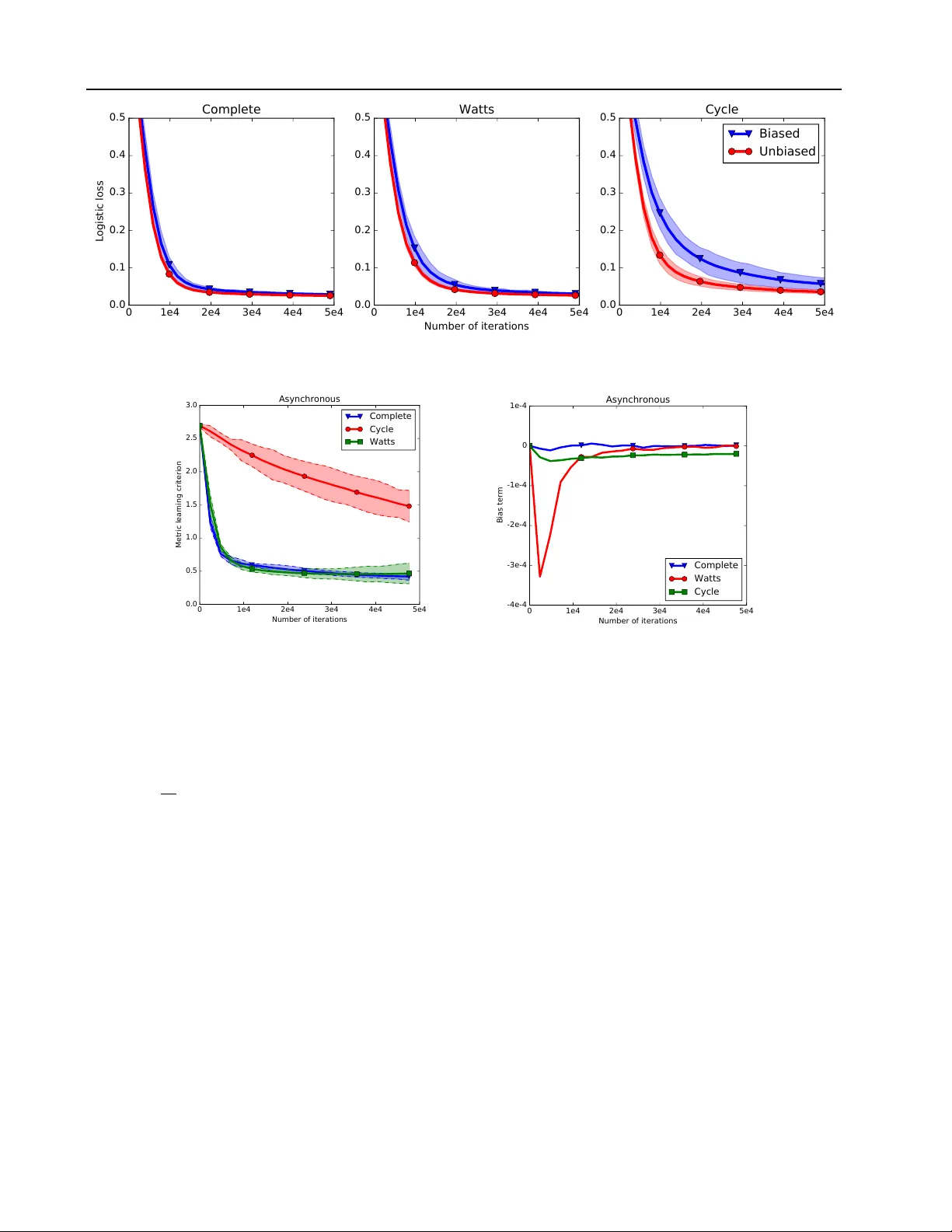
Gossip Dual A veraging f or Decentralized Optimization of Pairwise Functions Igor Colin I G O R . C O L I N @ T E L E C O M - P A R I S T E C H . F R L TCI, CNRS, T ´ el ´ ecom ParisT ech, Un versit ´ e Paris-Saclay , 75013 Paris, France A ur ´ elien Bellet AU R E L I E N . B E L L E T @ I N R I A . F R Magnet T eam, INRIA Lille – Nord Europe, 59650 V illeneuve d’Ascq, France Joseph Salmon J O S E P H . S A L M O N @ T E L E C O M - P A R I S T E C H . F R St ´ ephan Cl ´ emenc ¸ on S T E P H A N . C L E M E N C O N @ T E L E C O M - P A R I S T E C H . F R L TCI, CNRS, T ´ el ´ ecom ParisT ech, Un versit ´ e Paris-Saclay , 75013 Paris, France Abstract In decentralized networks (of sensors, connected objects, etc. ), there is an important need for ef fi- cient algorithms to optimize a global cost func- tion, for instance to learn a global model from the local data collected by each computing unit. In this paper, we address the problem of decen- tralized minimization of pairwise functions of the data points, where these points are distributed ov er the nodes of a graph defining the commu- nication topology of the network. This general problem finds applications in ranking, distance metric learning and graph inference, among oth- ers. W e propose new gossip algorithms based on dual av eraging which aims at solving such problems both in synchronous and asynchronous settings. The proposed frame work is flexible enough to deal with constrained and regularized variants of the optimization problem. Our the- oretical analysis rev eals that the proposed algo- rithms preserve the con v ergence rate of central- ized dual a veraging up to an additive bias term. W e present numerical simulations on Area Under the ROC Curve (A UC) maximization and metric learning problems which illustrate the practical interest of our approach. 1. Introduction The increasing popularity of large-scale and fully decen- tralized computational architectures, fueled for instance by Pr oceedings of the 33 rd International Confer ence on Machine Learning , New Y ork, NY , USA, 2016. JMLR: W&CP v olume 48. Copyright 2016 by the author(s). the advent of the “Internet of Things”, moti vates the de vel- opment of ef ficient optimization algorithms adapted to this setting. An important application is machine learning in wired and wireless networks of agents (sensors, connected objects, mobile phones, etc. ), where the agents seek to min- imize a global learning objectiv e which depends of the data collected locally by each agent. In such networks, it is typi- cally impossible to ef ficiently centralize data or to globally aggregate intermediate results: agents can only communi- cate with their immediate neighbors ( e .g., agents within a small distance), often in a completely asynchronous f ash- ion. Standard distributed optimization and machine learn- ing algorithms (implemented for instance using MapRe- duce/Spark) require a coordinator node and/or to maintain synchrony , and are thus unsuitable for use in decentralized networks. In contrast, gossip algorithms (Tsitsiklis, 1984; Boyd et al., 2006; Kempe et al., 2003; Shah, 2009) are tailored to this setting because they only rely on simple peer-to-peer communication: each agent only exchanges information with one neighbor at a time. V arious gossip algorithms hav e been proposed to solve the flagship problem of de- centralized optimization, namely to find a parameter vec- tor θ which minimizes an av erage of con vex functions (1 /n ) P n i =1 f ( θ ; x i ) , where the data x i is only known to agent i . The most popular algorithms are based on (sub)gradient descent (Johansson et al., 2010; Nedi ´ c & Ozdaglar, 2009; Ram et al., 2010; Bianchi & Jakubow- icz, 2013), ADMM (W ei & Ozdaglar, 2012; 2013; Iutzeler et al., 2013) or dual av eraging (Duchi et al., 2012; Y uan et al., 2012; Lee et al., 2015; Tsianos et al., 2015), some of which can also accommodate constraints or regulariza- tion on θ . The main idea underlying these methods is that each agent seeks to minimize its local function by applying local updates ( e.g., gradient steps) while exchanging infor- Gossip Dual A veraging f or Decentralized Optimization of Pairwise Functions mation with neighbors to ensure a global conv ergence to the consensus value. In this paper , we tackle the problem of minimizing an av- erage of pairwise functions of the agents’ data: min θ 1 n 2 X 1 ≤ i,j ≤ n f ( θ ; x i , x j ) . (1) This problem finds numerous applications in statistics and machine learning, e.g., Area Under the R OC Curve (A UC) maximization (Zhao et al., 2011), distance/similarity learn- ing (Bellet et al., 2015), ranking (Cl ´ emenc ¸ on et al., 2008), supervised graph inference (Biau & Bleakley, 2006) and multiple kernel learning (Kumar et al., 2012), to name a few . As a motiv ating e xample, consider a mobile phone ap- plication which locally collects information about its users. The provider could be interested in learning pairwise sim- ilarity functions between users in order to group them into clusters or to recommend them content without having to centralize data on a server (which would be costly for the users’ bandwidth) or to synchronize phones. The main difficulty in Problem (1) comes from the fact that each term of the sum depends on two agents i and j , mak- ing the local update schemes of previous approaches im- possible to apply unless data is exchanged between nodes. Although gossip algorithms hav e recently been introduced to ev aluate such pairwise functions for a fixed θ (Pelck- mans & Suykens, 2009; Colin et al., 2015), to the best of our kno wledge, efficiently finding the optimal solution θ in a decentralized way remains an open challenge. Our con- tributions to wards this objectiv e are as follows. W e propose new gossip algorithms based on dual av eraging (Nesterov, 2009; Xiao, 2010) to efficiently solve Problem (1) and its constrained or regularized v ariants. Central to our methods is a light data propagation scheme which allows the nodes to compute biased estimates of the gradients of functions in (1). W e then propose a theoretical analysis of our algo- rithms both in synchronous and asynchronous settings es- tablishing their con vergence under an additional hypothesis that the bias term decreases fast enough ov er the iterations (and we ha ve observed such a fast decrease in all our exper- iments). Finally , we present some numerical simulations on Area Under the R OC Curve (A UC) maximization and metric learning problems. These experiments illustrate the practical performance of the proposed algorithms and the influence of netw ork topology , and show that in practice the influence of the bias term is negligible as it decreases very fast with the number of iterations. The paper is organized as follows. Section 2 formally intro- duces the problem of interest and briefly revie ws the dual av eraging method, which is at the root of our approach. Section 3 presents the proposed gossip algorithms and their con vergence analysis. Section 4 displays our numerical simulations. Finally , concluding remarks are collected in Section 5. 2. Preliminaries 2.1. Definitions and Notation For any integer p > 0 , we denote by [ p ] the set { 1 , . . . , p } and by | F | the cardinality of any finite set F . W e denote an undirected graph by G = ( V , E ) , where V = [ n ] is the set of vertices and E ⊆ V × V is the set of edges. A node i ∈ V has degree d i = |{ j : ( i, j ) ∈ E }| . G is connected if for all ( i, j ) ∈ V 2 there exists a path connecting i and j ; it is bipartite if there exist S, T ⊂ V such that S ∪ T = V , S ∩ T = ∅ and E ⊆ ( S × T ) ∪ ( T × S ) . The graph Laplacian of G is denoted by L ( G ) = D ( G ) − A ( G ) , where D ( G ) and A ( G ) are respectiv ely the degree and the adjacency matri- ces of G . The transpose of a matrix M ∈ R n × n is denoted by M > . A matrix P ∈ R n × n is termed stochastic whenev er P ≥ 0 and P 1 n = 1 n , where 1 n = (1 , . . . , 1) > ∈ R n , and bi- stochastic whenever both P and P > are stochastic. W e denote by I n the identity matrix in R n × n , by ( e 1 , . . . , e n ) the canonical basis of R n , by I {E } the indicator function of any ev ent E and by k · k the usual ` 2 -norm. For θ ∈ R d and g : R d → R , we denote by ∇ g ( θ ) the gradient of g at θ . Finally , given a collection of vectors u 1 , . . . , u n , we denote by ¯ u n = (1 /n ) P n i =1 u i its empirical mean. 2.2. Problem Statement W e represent a network of n agents as an undirected graph G = ([ n ] , E ) , where each node i ∈ [ n ] corresponds to an agent and ( i, j ) ∈ E if nodes i and j can exchange infor- mation directly ( i.e . , they are neighbors). For ease of e xpo- sition, we assume that each node i ∈ [ n ] holds a single data point x i ∈ X . Though restrictive in practice, this assump- tion can easily be relaxed, b ut it w ould lead to more techni- cal details to handle the storage size, without changing the ov erall analysis (see supplementary material for details). Giv en d > 0 , let f : R d × X × X → R a differentiable and con vex function with respect to the first variable. W e assume that for any ( x, x 0 ) ∈ X 2 , there exists L f > 0 such that f ( · ; x, x 0 ) is L f -Lipschitz (with respect to the ` 2 -norm). Let ψ : R d → R + be a non-negativ e, con- ve x, possibly non-smooth, function such that, for simplic- ity , ψ (0) = 0 . W e aim at solving the following optimiza- tion problem: min θ ∈ R d 1 n 2 X 1 ≤ i,j ≤ n f ( θ ; x i , x j ) + ψ ( θ ) . (2) In a typical machine learning scenario, Problem (2) is a (regularized) empirical risk minimization problem and θ Gossip Dual A veraging f or Decentralized Optimization of Pairwise Functions Algorithm 1 Stochastic dual a veraging in the centralized setting Require: Step size ( γ ( t )) t ≥ 0 > 0 . 1: Initialization: θ = 0 , ¯ θ = 0 , z = 0 . 2: for t = 1 , . . . , T do 3: Update z ← z + g ( t ) , where E [ g ( t ) | θ ] = ∇ ¯ f n ( θ ) 4: Update θ ← π t ( z ) 5: Update ¯ θ ←  1 − 1 t  ¯ θ + 1 t θ 6: end for 7: return ¯ θ corresponds to the model parameters to be learned. The quantity f ( θ ; x i , x j ) is a pairwise loss measuring the per- formance of the model θ on the data pair ( x i , x j ) , while ψ ( θ ) represents a regularization term penalizing the com- plexity of θ . Common examples of re gularization terms in- clude indicator functions of a closed con vex set to model explicit con vex constraints, or norms enforcing specific properties such as sparsity (a canonical example being the ` 1 -norm). Many machine learning problems can be cast as Problem (2). For instance, in A UC maximization (Zhao et al., 2011), binary labels ( ` 1 , . . . , ` n ) ∈ {− 1 , 1 } n are assigned to the data points and we want to learn a (linear) scoring rule x 7→ x > θ which hopefully gives larger scores to positi ve data points than to negati ve ones. One may use the logistic loss f ( θ ; x i , x j ) = I { ` i >` j } log  1 + exp(( x j − x i ) > θ )  , and the re gularization term ψ ( θ ) can be the square ` 2 -norm of θ (or the ` 1 -norm when a sparse model is desired). Other popular instances of Problem (2) include metric learning (Bellet et al., 2015), ranking (Cl ´ emenc ¸ on et al., 2008), su- pervised graph inference (Biau & Bleakle y, 2006) and mul- tiple kernel learning (Kumar et al., 2012). For notational conv enience, we denote by f i the partial function (1 /n ) P n j =1 f ( · ; x i , x j ) for i ∈ [ n ] and by ¯ f n = (1 /n ) P n i =1 f i . Problem (2) can then be recast as: min θ ∈ R d R n ( θ ) = ¯ f n ( θ ) + ψ ( θ ) . (3) Note that the function ¯ f n is L f -Lipschitz, since all the f i are L f -Lipschitz. Remark 1. Throughout the paper we assume that the func- tion f is dif ferentiable, but we expect all our results to hold ev en when f is non-smooth, for instance in L 1 -regression problems or when using the hinge loss. In this case, one simply needs to replace gradients by subgradients in our algorithms, and a similar analysis could be performed. 2.3. Centralized Dual A veraging In this section, we re view the stochastic dual a veraging op- timization algorithm (Nestero v, 2009; Xiao, 2010) to solve Problem (2) in the centralized setting (where all data lie on the same machine). This method is at the root of our gos- sip algorithms, for reasons that will be made clear in Sec- tion 3. T o explain the main idea behind dual averaging, let us first consider the iterations of Stochastic Gradient De- scent (SGD), assuming ψ ≡ 0 for simplicity: θ ( t + 1) = θ ( t ) − γ ( t ) g ( t ) , where E [ g ( t ) | θ ( t )] = ∇ ¯ f n ( θ ( t )) , and ( γ ( t )) t ≥ 0 is a non- negati ve non-increasing step size sequence. For SGD to con verge to an optimal solution, the step size sequence must satisfy γ ( t ) − → t → + ∞ 0 and P ∞ t =0 γ ( t ) = ∞ . As no- ticed by Nesterov (2009), an undesirable consequence is that new gradient estimates are giv en smaller weights than old ones. Dual averaging aims at integrating all gradient estimates with the same weight. Let ( γ ( t )) t ≥ 0 be a positiv e and non-increasing step size sequence. The dual av eraging algorithm maintains a se- quence of iterates ( θ ( t )) t> 0 , and a sequence ( z ( t )) t ≥ 0 of “dual” v ariables which collects the sum of the unbiased gradient estimates seen up to time t . W e initialize to θ (1) = z (0) = 0 . At each step t > 0 , we compute an unbiased estimate g ( t ) of ∇ ¯ f n ( θ ( t )) . The most com- mon choice is to take g ( t ) = ∇ f ( θ ; x i t , x j t ) where i t and j t are drawn uniformly at random from [ n ] . W e then set z ( t + 1) = z ( t ) + g ( t ) and generate the next iterate with the following rule:    θ ( t + 1) = π ψ t ( z ( t + 1)) , π ψ t ( z ) := arg min θ ∈ R d  − z > θ + k θ k 2 2 γ ( t ) + tψ ( θ )  . When it is clear from the context, we will drop the depen- dence in ψ and simply write π t ( z ) = π ψ t ( z ) . Remark 2. Note that π t ( · ) is related to the proximal op- erator of a function φ : R d → R defined by prox φ ( x ) = arg min z ∈ R d  k z − x k 2 / 2 + φ ( x )  . Indeed, one can write: π t ( z ) = pro x tγ ( t ) ψ ( γ ( t ) z ) . For many functions ψ of practical interest, π t ( · ) has a closed form solution. For instance, when ψ = k · k 2 , π t ( · ) corresponds to a simple scaling, and when ψ = k · k 1 it is a soft-thresholding operator . If ψ is the indicator function of a closed conv ex set C , then π t ( · ) is the projection operator onto C . The dual averaging method is summarized in Algorithm 1. If γ ( t ) ∝ 1 / √ t then for any T > 0 : E T  R n ( ¯ θ ( T )) − R n ( θ ∗ )  = O (1 / √ T ) , where θ ∗ ∈ arg min θ ∈ R d R n ( θ ) , ¯ θ ( T ) = 1 T P T i =1 θ ( t ) is the av eraged iterate and E T is the expectation o ver all pos- sible sequences ( g ( t )) 1 ≤ t ≤ T . A precise statement of this Gossip Dual A veraging f or Decentralized Optimization of Pairwise Functions result along with a proof can be found in the supplemen- tary material for completeness. Notice that dual av eraging cannot be easily adapted to our decentralized setting. Indeed, a node cannot compute an unbiased estimate of its gradient: this would imply an ac- cess to the entire set of data points, which violates the com- munication and storage constraints. Therefore, data points hav e to be appropriately propagated during the optimiza- tion procedure, as detailed in the following section. 3. Pairwise Gossip Dual A veraging W e no w turn to our main goal, namely to develop efficient gossip algorithms for solving Problem (2) in the decentral- ized setting. The methods we propose rely on dual aver - aging (see Section 2.3). This choice is guided by the fact that the structure of the updates makes dual averaging much easier to analyze in the distributed setting than sub-gradient descent when the problem is constrained or regularized. This is because dual averaging maintains a simple sum of sub-gradients, while the (non-linear) smoothing operator π t is applied separately . Our work builds upon the analysis of Duchi et al. (2012), who proposed a distributed dual averaging algorithm to optimize an average of univariate functions f ( · ; x i ) . In their algorithm, each node i computes unbiased estimates of its local function ∇ f ( · ; x i ) that are iteratively aver - aged over the network. Unfortunately , in our setting, the node i cannot compute unbiased estimates of ∇ f i ( · ) = ∇ (1 /n ) P n j =1 f ( · ; x i , x j ) : the latter depends on all data points while each node i ∈ [ n ] only holds x i . T o go around this problem, we rely on a gossip data propagation step (Pelckmans & Suykens, 2009; Colin et al., 2015) so that the nodes are able to compute biased estimates of ∇ f i ( · ) while keeping the communication and memory overhead to a small lev el for each node. W e present and analyze our algorithm in the synchronous setting in Section 3.1. W e then turn to the more intricate analysis of the asynchronous setting in Section 3.2. 3.1. Synchronous Setting In the synchronous setting, we assume that each node has access to a global clock such that ev ery node can update simultaneously at each tick of the clock. Although not very realistic, this setting allo ws for simpler analysis. W e as- sume that the scaling sequence ( γ ( t )) t ≥ 0 is the same for ev ery node. At an y time, each node i has the following quantities in its local memory register: a v ariable z i (the gradient accumulator), its original observation x i , and an auxiliary observation y i , which is initialized at x i but will change throughout the algorithm as a result of data propa- gation. Algorithm 2 Gossip dual av eraging for pairwise function in synchronous setting Require: Step size ( γ ( t )) t ≥ 1 > 0 . 1: Each node i initializes y i = x i , z i = θ i = ¯ θ i = 0 . 2: for t = 1 , . . . , T do 3: Draw ( i, j ) uniformly at random from E 4: Set z i , z j ← z i + z j 2 5: Swap auxiliary observ ations: y i ↔ y j 6: for k = 1 , . . . , n do 7: Update z k ← z k + ∇ θ f ( θ k ; x k , y k ) 8: Compute θ k ← π t ( z k ) 9: A v erage ¯ θ k ←  1 − 1 t  ¯ θ k + 1 t θ k 10: end for 11: end for 12: return Each node k has ¯ θ k The algorithm goes as follows. At each iteration, an edge ( i, j ) ∈ E of the graph is drawn uniformly at random. Then, nodes i and j average their gradient accumulators z i and z j , and swap their auxiliary observations y i and y j . Fi- nally , e very node of the netw ork performs a dual a veraging step, using their original observ ation and their current aux- iliary one to estimate the partial gradient. The procedure is detailed in Algorithm 2, and the following proposition adapts the conv ergence rate of centralized dual averaging under the hypothesis that the contribution of the bias term decreases fast enough ov er the iterations. Theorem 1. Let G be a connected and non-bipartite gr aph with n nodes, and let θ ∗ ∈ arg min θ ∈ R d R n ( θ ) . Let ( γ ( t )) t ≥ 1 be a non-increasing and non-ne gative sequence. F or any i ∈ [ n ] and any t ≥ 0 , let z i ( t ) ∈ R d and ¯ θ i ( t ) ∈ R d be generated according to Algorithm 2. Then for any i ∈ [ n ] and T > 1 , we have: E T [ R n ( ¯ θ i ) − R n ( θ ∗ )] ≤ C 1 ( T ) + C 2 ( T ) + C 3 ( T ) , wher e                            C 1 ( T ) = 1 2 T γ ( T ) k θ ∗ k 2 + L 2 f 2 T T − 1 X t =1 γ ( t ) , C 2 ( T ) = 3 L 2 f T  1 − q λ G 2  T − 1 X t =1 γ ( t ) , C 3 ( T ) = 1 T T − 1 X t =1 E t [( ω ( t ) − θ ∗ ) > ¯  n ( t )] , and λ G 2 < 1 is the second lar gest eigen value of the matrix W ( G ) = I n − 1 | E | L ( G ) . Sketch of pr oof. First notice that at a gi ven (outer) iteration t + 1 , ¯ z n is updated as follows: ¯ z n ( t + 1) = ¯ z n ( t ) + 1 n n X k =1 d k ( t ) , (4) Gossip Dual A veraging f or Decentralized Optimization of Pairwise Functions where d k ( t ) = ∇ θ f ( θ k ( t ); x k , y k ( t + 1)) is a biased esti- mate of ∇ f k ( θ k ( t )) . Let  k ( t ) = d k ( t ) − g k ( t ) be the bias, so that we hav e E [ g k ( t ) | θ k ( t )] = ∇ f k ( θ k ( t )) . Let us define ω ( t ) = π t ( ¯ z n ( t )) . Using conv exity of R n , the gradient’ s definition and the fact that the functions ¯ f n and π t are both L f -Lipschitz, we obtain: for T ≥ 2 and i ∈ [ n ] , E T [ R n ( ¯ θ i ( T )) − R n ( θ ∗ )] ≤ L f nT T X t =2 γ ( t − 1) n X j =1 E t h k z i ( t ) − z j ( t ) k i (5) + L f nT T X t =2 γ ( t − 1) n X j =1 E t h k ¯ z n ( t ) − z j ( t ) k i (6) + 1 T T X t =2 E t [( ω ( t ) − θ ∗ ) > ¯ g n ( t )] . (7) Using Lemma 4 (see supplementary material), the terms (5)-(6) can be bounded by C 2 ( T ) . The term (7) requires a specific analysis because the updates are performed using biased estimates. W e decompose it as follows: 1 T T X t =2 E t h ω ( t ) − θ ∗ ) > ¯ g n ( t ) i = 1 T T X t =2 E t h ( ω ( t ) − θ ∗ ) > ( ¯ d n ( t ) − ¯  n ( t )) i ≤ 1 T T X t =2 E t h ( ω ( t ) − θ ∗ ) > ¯ d n ( t ) i (8) + 1 T T X t =2 E t h ( ω ( t ) − θ ∗ ) > ¯  n ( t ) i . The term (8) can be bounded by C 1 ( T ) (see Xiao, 2010, Lemma 9). W e refer the reader to the supplementary mate- rial for the detailed proof. The rate of con vergence in Proposition 1 is divided into three parts: C 1 ( T ) is a data dependent term which corre- sponds to the rate of con ver gence of the centralized dual av eraging, while C 2 ( T ) and C 3 ( T ) are network dependent terms since 1 − λ G 2 = β G n − 1 / | E | , where β G n − 1 is the sec- ond smallest eigenv alue of the graph Laplacian L ( G ) , also known as the spectral gap of G . The con vergence rate of our algorithm thus improves when the spectral gap is large, which is typically the case for well-connected graphs (Chung, 1997). Note that C 2 ( T ) corresponds to the net- work dependence for the distrib uted dual a veraging algo- rithm of Duchi et al. (2012) while the term C 3 ( T ) comes from the bias of our partial gradient estimates. In practice, C 3 ( T ) v anishes quickly and has a small impact on the rate of con vergence, as sho wn in Section 4. Algorithm 3 Gossip dual av eraging for pairwise function in asynchronous setting Require: Step size ( γ ( t )) t ≥ 0 > 0 , probabilities ( p k ) k ∈ [ n ] . 1: Each node i initializes y i = x i , z i = θ i = ¯ θ i = 0 , m i = 0 . 2: for t = 1 , . . . , T do 3: Draw ( i, j ) uniformly at random from E 4: Swap auxiliary observ ations: y i ↔ y j 5: for k ∈ { i, j } do 6: Set z k ← z i + z j 2 7: Update z k ← 1 p k ∇ θ f ( θ k ; x k , y k ) 8: Increment m k ← m k + 1 p k 9: Compute θ k ← π m k ( z k ) 10: A v erage ¯ θ k ←  1 − 1 m k p k  ¯ θ k 11: end for 12: end for 13: return Each node k has ¯ θ k 3.2. Asynchronous Setting For any variant of gradient descent over a network with a decreasing step size, there is a need for a common time scale to perform the suitable decrease. In the synchronous setting, this time scale information can be shared easily among nodes by assuming the av ailability of a global clock. This is con venient for theoretical considerations, but is un- realistic in practical (asynchronous) scenarios. In this sec- tion, we place ourselves in a fully asynchronous setting where each node has a local clock, ticking at a Poisson rate of 1 , independently from the others. This is equiv alent to a global clock ticking at a rate n Poisson process which wakes up an edge of the network uniformly at random (see Boyd et al., 2006, for details on clock modeling). W ith this in mind, Algorithm 2 needs to be adapted to this setting. First, one cannot perform a full dual av eraging up- date over the network since only two nodes wake up at each iteration. Also, as mentioned earlier , each node needs to maintain an estimate of the current iteration number in or- der for the scaling factor γ to be consistent across the net- work. For k ∈ [ n ] , let p k denote the probability for the node k to be pick ed at an y iteration. If the edges are picked uniformly at random, then one has p k = 2 d k / | E | . For sim- plicity , we focus only on this case, although our analysis holds in a more general setting. Let us define an activ ation v ariable ( δ k ( t )) t ≥ 1 such that for any t ≥ 1 , δ k ( t ) = ( 1 if node k is picked at iteration t, 0 otherwise . One can immediately see that ( δ k ( t )) t ≥ 1 are i.i.d. random variables, Bernoulli distributed with parameter p k . Let us define ( m k ( t )) ≥ 0 such that m k (0) = 0 and for t ≥ 0 , m k ( t + 1) = m k ( t ) + δ k ( t +1) p k . Since ( δ k ( t )) t ≥ 1 are Gossip Dual A veraging f or Decentralized Optimization of Pairwise Functions Bernoulli random variables, m k ( t ) is an unbiased estimate of the time t . Using this estimator, we can now adapt Algorithm 2 to the fully asynchronous case, as shown in Algorithm 3. The up- date step slightly dif fers from the synchronous case: the partial gradient has a weight 1 /p k instead of 1 so that all partial functions asymptotically count in equal way in e very gradient accumulator . In contrast, uniform weights would penalize partial gradients from low degree nodes since the probability of being drawn is proportional to the degree. This weighting scheme is essential to ensure the conv er- gence to the global solution. The model av eraging step also needs to be altered: in absence of an y global clock, the weight 1 /t cannot be used and is replaced by 1 / ( m k p k ) , where m k p k corresponds to the average number of times that node k has been selected so far . The following result is the analogous of Theorem 1 for the asynchronous setting. Theorem 2. Let G be a connected and non bipartite graph. Let ( γ ( t )) t ≥ 1 be defined as γ ( t ) = c/t 1 / 2+ α for some constant c > 0 and α ∈ (0 , 1 / 2) . F or i ∈ [ n ] , let ( d i ( t )) t ≥ 1 , ( g i ( t )) t ≥ 1 , (  i ( t )) t ≥ 1 , ( z i ( t )) t ≥ 1 and ( θ i ( t )) t ≥ 1 be generated as described in Algorithm 3. Then, ther e exists some constant C < + ∞ suc h that, for θ ∗ ∈ arg min θ 0 ∈ R d R n ( θ 0 ) , i ∈ [ n ] and T > 0 , R n ( ¯ θ i ( T )) − R n ( θ ∗ ) ≤ C max( T − α/ 2 , T α − 1 / 2 ) + 1 T T X t =2 E t [( ω ( t ) − θ ∗ ) >  n ( t )] . The proof is giv en in the supplementary material. Remark 3. In the asynchronous setting, no con vergence rate was kno wn ev en for the distributed dual averaging al- gorithm of Duchi et al. (2012), which deals with the sim- pler problem of minimizing univariate functions. The ar- guments used to deri ve Theorem 2 can be adapted to de- riv e a con ver gence rate (without the bias term) for an asyn- chronous version of their algorithm. Remark 4. W e hav e focused on the setting where all pairs of observations are inv olved in the objectiv e. In practice, the objectiv e may depend only on a subset of all pairs. T o efficiently apply our algorithm to this case, one should tak e advantage of the potential structure of the subset of inter- est: for instance, one could attach some additional concise information to each observation so that a node can easily identify whether a pair contributes to the objectiv e, and if not set the loss to be zero. This is essentially the case in the A UC optimization problem studied in Section 4, where pairs of similarly labeled observations do not contribute to the objecti ve. If the subset of pairs cannot be e xpressed in such a compact form, then one w ould need to provide each node with an index list of acti ve pairs, which could be memory-intensiv e when n is large. 4. Numerical Simulations In this section, we present numerical experiments on two popular machine learning problems in volving pairwise functions: Area Under the R OC Curve (A UC) maximiza- tion and metric learning. Our results show that our al- gorithms con verge and that the bias term vanishes very quickly with the number of iterations. T o study the influence of the netw ork topology , we perform our simulations on three types of network (see T able 1 for the corresponding spectral gap v alues): • Complete graph: All nodes are connected to each other . It is the ideal situation in our frame- work, since any pair of nodes can communicate di- rectly . In this setting, the bias of gradient esti- mates should be very small, as one has for any k ∈ [ n ] and any t ≥ 1 , E t [ d k ( t ) | θ k ( t )] = 1 / ( n − 1) P y 0 6 = y k ( t ) ∇ θ f ( θ k ( t ); x k , y 0 ) . For a network size n , the complete graph achie ves the highest spectral gap: 1 − λ G 2 = 1 /n , see Bollob ´ as (1998, Ch.9) or Chung (1997, Ch.1) for details. • Cycle graph: This is the worst case in terms of con- nectivity: each node only has two neighbors. This network has a spectral gap of order 1 /n 3 , and giv es a lower bound in terms of con v ergence rate. • W atts-Str ogatz: This random network generation technique (W atts & Strogatz, 1998) relies on two pa- rameters: the average degree of the network k and a rewiring probability p . In expectation, the higher the rewiring probability , the better the connectivity of the network. Here, we use k = 5 and p = 0 . 3 to achiev e a compromise between the connectivities of the com- plete graph and the cycle graph. A UC Maximization W e first present an application of our algorithms to A UC maximization on a real dataset. Giv en a set of data points x 1 , . . . , x n ∈ R d with associ- ated binary labels ` 1 , . . . , ` n ∈ {− 1 , 1 } , the goal is to learn a linear scoring rule x 7→ x > θ parameterized by θ ∈ R d which maximizes: AU C ( θ ) = P 1 ≤ i,j ≤ n I { ` i >` j } I { x > i θ>x > j θ } P 1 ≤ i,j ≤ n I { ` i >` j } . It corresponds to the probability that the scoring rule asso- ciated with θ outputs a higher score on a positively labeled sample than on a negati vely labeled one. This formulation leads to a non-smooth optimization problem; therefore, one Gossip Dual A veraging f or Decentralized Optimization of Pairwise Functions Dataset Complete graph W atts-Strogatz Cycle graph Breast Cancer (A UC Maximization, n = 699 ) 1 . 43 · 10 − 3 8 . 71 · 10 − 5 5 . 78 · 10 − 8 Synthetic (Metric Learning, n = 1000 ) 1 . 00 · 10 − 3 6 . 23 · 10 − 5 1 . 97 · 10 − 8 T able 1. Spectral gap values 1 − λ G 2 for each network. (a) Evolution of the objective function and its standard deviation (synchronous) 0 1e4 2e4 3e4 4e4 5e4 Number of iterations 0.0 0.1 0.2 0.3 0.4 0.5 Logistic loss Asynchronous Complete Cycle Watts (b) Evolution of the objective function and its standard de viation (asynchronous) 0 1e4 2e4 3e4 4e4 5e4 Number of iterations -1e-3 0 1e-3 2e-3 3e-3 4e-3 5e-3 Bias term Asynchronous Complete Watts Cycle (c) Evolution of the bias term (asyn- chronous) Figure 1. A UC maximization in synchronous and asynchronous settings. typically minimizes a con vex surrogate such as the logistic loss: R n ( θ ) = 1 n 2 X 1 ≤ i,j ≤ n I { ` i >` j } log  1 + exp(( x j − x i ) > θ )  . W e do not apply any regularization ( i.e. , ψ ≡ 0 ), and use the Breast Cancer Wisconsin dataset, 1 which consists of n = 699 points in d = 11 dimensions. W e initialize each θ i to 0 and for each network, we run 50 times Algorithms 2 and 3 with γ ( t ) = 1 / √ t . 2 Figure 1(a) shows the e volution of the objective function and the asso- ciated standard de viation (across nodes) with the number of iterations in the synchronous setting. As expected, the av erage con ver gence rate on the complete and the W atts- Strogatz networks is much better than on the poorly con- nected cycle network. The standard deviation of the node estimates also decreases with the connecti vity of the net- work. The results for the asynchronous setting are shown in Fig- ure 1(b). As expected, the con ver gence rate is slower in terms of number of iterations (roughly 5 times) than in the synchronous setting. Note howe ver that much fewer dual av eraging steps are performed: for instance, on the W atts- Strogatz network, reaching a 0 . 1 loss requires 210 , 000 1 https://archive.ics.uci.edu/ml/datasets/ Breast+Cancer+Wisconsin+(Original) 2 Even if this scaling sequence does not fulfill the hypothesis of Theorem 2 for the asynchronous setting, the con vergence rate is acceptable in practice. (partial) gradient computations in the synchronous setting and only 25 , 000 in the asynchronous setting. Moreov er , the standard deviation of the estimates is much lower than in the synchronous setting. This is because communica- tion and local optimization are better balanced in the asyn- chronous setting (one optimization step for each gradient accumulator averaged) than in the synchronous setting ( n optimization steps for 2 gradient accumulators av eraged). The good practical con vergence of our algorithm comes from the fact that the bias term  n ( t ) > ω ( t ) vanishes quite fast. Figure 1(c) sho ws that its average v alue quickly con verges to 0 on all networks. Moreover , its order of magnitude is negligible compared to the objective func- tion. In order to fully estimate the impact of this bias term on the performance, we also compare our algorithm to the ideal but unrealistic situation where each node is giv en an unbiased estimate of its partial gradient: instead of adding ∇ f ( θ i ( t ); x i , y i ( t )) to z i ( t ) , a node i will add ∇ f ( θ i ( t ); x i , x j ) where j ∈ [ n ] is picked uniformly at ran- dom. As shown in Figure 2, the performance of both meth- ods are very similar on well-connected networks. Metric Learning W e now turn to a metric learning ap- plication. W e consider the family of Mahalanobis dis- tances D θ ( x i , x j ) = ( x i − x j ) > θ ( x i − x j ) parameter- ized by θ ∈ S d + , where S d + is the cone of d × d posi- tiv e semi-definite real-valued matrices. Gi ven a set of data points x 1 , . . . , x n ∈ R d with associated labels ` 1 , . . . , ` n ∈ {− 1 , 1 } , the goal is to find θ ∈ S d + which minimizes the Gossip Dual A veraging f or Decentralized Optimization of Pairwise Functions 0 1e4 2e4 3e4 4e4 5e4 0.0 0.1 0.2 0.3 0.4 0.5 Logi stic los s Compl ete 0 1e4 2e4 3e4 4e4 5e4 Number of i teratio ns 0.0 0.1 0.2 0.3 0.4 0.5 Watts 0 1e4 2e4 3e4 4e4 5e4 0.0 0.1 0.2 0.3 0.4 0.5 Cycl e Bias ed Unbi ased Figure 2. A UC maximization: comparison between our algorithm and an unbiased version. 0 1e4 2e4 3e4 4e4 5e4 Number of i teratio ns 0.0 0.5 1.0 1.5 2.0 2.5 3.0 Metric lear ning cri ter ion Asyn chron ous Compl ete Cycl e Watts (a) Evolution of the objectiv e function and its stan- dard deviation (asynchronous setting) 0 1e4 2e4 3e4 4e4 5e4 Number of iterations -4e-4 -3e-4 -2e-4 -1e-4 0 1e-4 Bias term Asynchronous Complete Watts Cycle (b) Evolution of the bias term Figure 3. Metric learning experiments. following criterion (Jin et al., 2009): R n ( θ ) = 1 n 2 X 1 ≤ i,j ≤ n  ` i ` j ( b − D θ ( x i , x j ))  + + ψ ( θ ) , where [ u ] + = max(0 , 1 − u ) , b > 0 , and ψ ( θ ) = ∞ if θ / ∈ S d + and 0 otherwise. W e use a synthetic dataset of n = 1 , 000 points generated as follo ws: each point is drawn from a mixture of 10 Gaussians in R 40 (each corre- sponding to a class) with all Gaussian means contained in a 5d subspace and their shared cov ariance matrix propor- tional to the identity with a variance factor such that some ov erlap is observed. Figure 3(a) sho ws the ev olution of the objecti ve function and its standard deviation for the asynchronous setting. As in the case of A UC maximization, the algorithm conv erges much faster on the well-connected networks than on the cycle network. Again, we can see in Figure 3(b) that the bias vanishes v ery quickly with the number of iterations. Additional Experiment W e refer to the supplementary material for a metric learning experiment on a real dataset. 5. Conclusion In this work, we have introduced new synchronous and asynchronous gossip algorithms to optimize functions de- pending on pairs of data points distributed over a network. The proposed methods are based on dual av eraging and can readily accommodate various popular regularization terms. W e provided an analysis showing that they behave similarly to the centralized dual av eraging algorithm, with additional terms reflecting the network connectivity and the gradient bias. Finally , we proposed some numerical experiments on A UC maximization and metric learning which illustrate the performance of the proposed algorithms, as well as the in- fluence of network topology . A challenging line of future research consists in designing and analyzing no vel adap- tiv e gossip schemes, where the communication scheme is dynamic and depends on the network connectivity proper- ties and on the local information carried by each node. Gossip Dual A veraging f or Decentralized Optimization of Pairwise Functions A. Outline of the Supplementary Material The supplementary material is organized as follows. In Section B, we recall the standard proof of con vergence rate for the (centralized) dual averaging. Then, in Section C, we impro ve the analysis of the decentralized v ersion of the dual av eraging algorithm for simple sums of functions, and provide insights to analyze the case of sum of pairwise functions. Our asynchronous variant is inv estigated in Section D. T echnical details on how to extend our framew ork to the case with multiple points per node are giv en in Section E. Finally , additional numerical results are discussed in Section F. B. Centralized Dual A veraging B.1. Deterministic Setting W e introduce the dual averaging algorithm for minimizing the sum f + ψ , in a context where f is con vex and smooth, ψ (0) = 0 , ψ is con vex, non-negati ve and possibly non-smooth, with a proximity operator simple to compute. In the centralized framew ork, this algorithm reads as follows: θ ( t + 1) = arg min θ 0 ∈ R d ( θ 0> t X s =1 g ( s ) + k θ 0 k 2 2 γ ( t ) + tψ ( θ 0 ) ) , (9) for any t ≥ 1 , where γ ( t ) represents a scale factor similar to a gradient step size use in standard gradient descent algorithms, and g ( t ) is a sequence of gradient of f taken at θ ( t ) . Moreover we initialize θ (1) = 0 . The function f we consider is here of the form ¯ f n ( θ ) = 1 /n P n i =1 f i ( θ ) , where each f i is assumed L f -Lipschitz for simplicity (so is f then). W e denote R n = ¯ f n + ψ . As a reminder, note that the Centralized dual a veraging method is explicitly stated in Algorithm 4. This particular formulation was introduced in (Xiao, 2009; 2010), extending the method introduced by (Nestero v, 2009) in the specific case of indicator functions. In this work, we borro w the notation from (Xiao, 2010). In order to perform a theoretical analysis of this algorithm, we introduce the following functions. Let us define, for t ≥ 0 V t ( z ) := max θ ∈ R d  z > θ − k θ k 2 2 γ ( t ) − tψ ( θ )  . Remark that with the assumption that ψ (0) = 0 , then V t (0) = 0 . W e also define the smoothing function π t that plays a crucial role in the dual algorithm formulation: π t ( z ) := arg max θ ∈ R d  z > θ − k θ k 2 2 γ ( t ) − tψ ( θ )  = arg min θ ∈ R d  − z > θ + k θ k 2 2 γ ( t ) + tψ ( θ )  Strong con vexity in θ of the objectiv e function, ensures that the solution of the optimization problem is unique. The following lemma links the function V t and the algorithm update and is a simple application of the results from (Xiao, 2009, Lemma 10): Lemma 1. F or any z ∈ R d , one has: π t ( z ) = ∇ V t ( z ) , (10) and the following statements hold true: for any z 1 , z 2 ∈ R d k π t ( z 1 ) − π t ( z 2 ) k ≤ γ ( t ) k z 1 − z 2 k , (11) and for any g , z ∈ R d , V t ( z + g ) ≤ V t ( z ) + g > ∇ V t ( z ) + γ ( t ) 2 k g k 2 . (12) W ith this notation one can write the dual av eraging rule as θ ( t + 1) = π t ( − z ( t + 1)) , where z ( t ) := P t − 1 s =1 g ( s ) , with the con vention z (1) = 0 . Moreover , adapting (Xiao, 2009, Lemma 11) we can state: Gossip Dual A veraging f or Decentralized Optimization of Pairwise Functions Algorithm 4 Centralized dual av eraging Require: Step size ( γ ( t )) t ≥ 1 > 0 . 1: Initialization θ = 0 , ¯ θ = 0 , z = 0 . 2: for t = 1 , . . . , T do 3: Update z ← z + g ( t ) , where g ( t ) = ∇ ¯ f n ( θ ) 4: Update θ ← π t ( z ) 5: Update ¯ θ ←  1 − 1 t  ¯ θ + 1 t θ 6: end for 7: return ¯ θ Lemma 2. F or any t ≥ 1 and any non-incr easing sequence ( γ ( t )) t ≥ 1 , we have V t ( − z ( t + 1)) + ψ ( θ ( t + 1)) ≤ V t − 1 ( − z ( t + 1)) . (13) W e also need a last technical result that we will use sev eral times in the following: Lemma 3. Let θ ( t ) = π t ( P t − 1 s =1 g ( s )) , and let ( γ ( t )) t ≥ 1 be a non-increasing and non-ne gative sequence sequence (with the con vention γ (0) = 0 ), then for any θ ∈ R d : 1 T T X t =1 g ( t ) > ( θ ( t ) − θ ) + 1 T T X t =1 ( ψ ( θ ( t )) − ψ ( θ )) ≤ 1 T T X t =1 γ ( t − 1) 2 k g ( t ) k 2 + k θ k 2 2 T γ ( T ) . (14) Pr oof. Use the definition of V T to get the following upper bound 1 T T X t =1 g ( t ) > ( θ ( t ) − θ ) + 1 T T X t =1 ( ψ ( θ ( t )) − ψ ( θ )) = 1 T T X t =1 g ( t ) > θ ( t ) + ψ ( θ ( t )) + k θ k 2 2 T γ ( T ) − ψ ( θ ) −  z ( T + 1) T  > θ − k θ k 2 2 T γ ( T ) ≤ 1 T T X t =1  g ( t ) > θ ( t ) + ψ ( θ ( t ))  + k θ ∗ k 2 2 T γ ( T ) + V T ( − z ( T + 1)) . (15) Then one can check that with (12) and Lemma 2 that: V t ( − z ( t + 1)) + ψ ( θ ( t + 1)) ≤ V t − 1 ( − z ( t + 1)) = V t − 1 ( − z ( t ) − g ( t )) ≤ V t − 1 ( − z ( t )) − g ( t ) > ∇ V t − 1 ( − z ( t )) + γ ( t − 1) 2 k g ( t ) k 2 = V t − 1 ( − z ( t )) − g ( t ) > θ ( t ) + γ ( t − 1) 2 k g ( t ) k 2 . From the last display , the follo wing holds: g ( t ) > θ ( t ) + ψ ( θ ( t + 1)) ≤ V t − 1 ( − z ( t )) − V t ( − z ( t + 1)) + γ ( t − 1) 2 k g ( t ) k 2 . Summing the former for t = 1 , . . . , T yields T X t =1 g ( t ) > θ ( t ) + ψ ( θ ( t + 1)) ≤ V 0 ( − s 0 ) − V T ( − s T ) + T X t =1 γ ( t − 1) 2 k g t k 2 . Gossip Dual A veraging f or Decentralized Optimization of Pairwise Functions Remark that V 0 (0) = 0 and ψ ( θ (1)) − ψ ( θ ( T + 1)) = − ψ ( θ ( T + 1)) ≤ 0 , so the previous display can be reduced to: T X t =1 g ( t ) > θ ( t ) + ψ ( θ ( t )) + V T ( − z ( T + 1)) ≤ T X t =1 γ ( t − 1) 2 k g ( t ) k 2 . (16) Combining with (15), the lemma holds true. Bounding the error of the dual av eraging is provided in the next theorem, where we remind that R n = ¯ f n + ψ : Theorem 3. Let ( γ ( t )) t ≥ 1 be a non increasing sequence. Let ( z ( t )) t ≥ 1 , ( θ ( t )) t ≥ 1 , ( ¯ θ ( t )) t ≥ 1 and ( g ( t )) t ≥ 1 be generated accor ding to Algorithm 4. Assume that the function ¯ f n is L f -Lipschitz and that θ ∗ ∈ arg min θ 0 ∈ R d R n ( θ 0 ) , then for any T ≥ 2 , one has: R n ( ¯ θ ( T )) − R n ( θ ∗ ) ≤ k θ ∗ k 2 2 T γ ( T ) + L 2 f 2 T T − 1 X t =1 γ ( t ) . (17) Mor eover , if one knows D > 0 suc h that k θ ∗ k ≤ D , then for the choice γ ( t ) = D L f √ 2 t , one has: R n ( ¯ θ ( T )) − R n ( θ ∗ ) ≤ √ 2 D L f √ T . Pr oof. Let T ≥ 2 . Using the conv exity of ¯ f n and ψ , we can get: R n ( ¯ θ ( T )) − R n ( θ ∗ ) ≤ 1 T T X t =1 ¯ f n ( θ ( t )) − ¯ f n ( θ ∗ ) + ψ ( ¯ θ ) − ψ ( θ ∗ ) ≤ 1 T T X t =1 g ( t ) > ( θ ( t ) − θ ∗ ) + 1 T T X t =1 ( ψ ( θ ( t )) − ψ ( θ ∗ )) ≤ 1 T T X t =1 γ ( t − 1) 2 k g ( t ) k 2 + k θ k 2 2 T γ ( T ) . where the second inequality holds since g ( t ) = ∇ ¯ f n ( θ ( t )) , and the third one is from an application of Lemma 3 with the choice θ = θ ∗ . Provided that k g ( t ) k ≤ L f , which is true whenev er ¯ f n is L f -Lipschitz. B.2. Stochastic Dual A veraging Similarly to sub-gradient descent algorithms, one can adapt dual averaging algorithm to a stochastic setting; this was studied extensiv ely by Xiao (2009). Instead of updating the dual variable z ( t ) with the (full) gradient of ¯ f n at θ ( t ) , one now only requires the e xpected value of the update to be the gradient, as detailed in Algorithm 1. As in the gradient descent case, con vergence results still hold in e xpectation, as stated in Theorem 4. Theorem 4. Let ( γ ( t )) t ≥ 1 be a non increasing sequence. Let ( z ( t )) t ≥ 1 , ( θ ( t )) t ≥ 1 and ( g ( t )) t ≥ 1 be generated accor ding to Algorithm 1. Assume that the function ¯ f n is L f -Lipschitz and that θ ∗ ∈ arg min θ 0 ∈ R d R n ( θ 0 ) , then for any T ≥ 2 , one has: E T h R n ( ¯ θ ( T )) − R n ( θ ∗ ) i ≤ k θ ∗ k 2 2 T γ ( T ) + L 2 f 2 T T − 1 X t =1 γ ( t ) , (18) wher e E T is the expectation o ver all possible sequence ( g ( t )) 1 ≤ t ≤ T . Mor eover , if one knows that D > 0 suc h that k θ ∗ k ≤ D , then for γ ( t ) = D L f √ 2 t , one has: E T  R n ( ¯ θ ( T )) − R n ( θ ∗ )  ≤ √ 2 D L f √ T . Gossip Dual A veraging f or Decentralized Optimization of Pairwise Functions Pr oof. One only has to prove that the conv exity inequality in Lemma 3 holds in expectation. The rest of the proof can be directly adapted from Theorem 3. Let T ≥ 2 ; using the con vexity of ¯ f n , one obtains: E T [ ¯ f n ( ¯ θ ( T )) − ¯ f n ( θ ∗ )] ≤ 1 T T X t =1 E T [ ¯ f n ( θ ( t )) − ¯ f n ( θ ∗ )] . For an y 0 < t ≤ T , E [ θ ( t ) | g (0) , . . . , g ( t − 1)] = θ ( t ) . Therefore, we have: E T [ ¯ f n ( θ ( t )) − ¯ f n ( θ ∗ )] = E t − 1 [ ¯ f n ( θ ( t )) − ¯ f n ( θ ∗ )] . The vector E t [ g ( t ) | θ ( t )] is the gradient of ¯ f n at θ ( t ) , we can then use ¯ f n con vexity to write: E t − 1 [ ¯ f n ( θ ( t )) − ¯ f n ( θ ∗ )] ≤ E t − 1 h ( θ ( t ) − θ ∗ ) > E t [ g ( t ) | θ ( t )] i . Using properties of conditional expectation, we obtain: E t − 1 h ( θ ( t ) − θ ∗ ) > E t [ g ( t ) | θ ( t )] i = E t − 1 h E t [( θ ( t ) − θ ∗ ) > g ( t ) | θ ( t )] i = E t [( θ ( t ) − θ ∗ ) > g ( t )] . Finally , we can write: E T [ ¯ f n ( ¯ θ ( T ) − f ( θ ∗ )] ≤ 1 T T X t =1 E t [( θ ( t ) − θ ∗ ) > g ( t )] = E T " 1 T T X t =1 ( θ ( t ) − θ ∗ ) > g ( t ) # . (19) C. Con vergence Pr oof for Synchr onous Pairwise Gossip Dual A veraging In (Duchi et al., 2012), the following con v ergence rate for distributed dual a veraging is established: R n ( ¯ θ i ( T )) − R n ( θ ∗ ) ≤ 1 2 T γ ( T ) k θ ∗ k 2 + L 2 f 2 T T X t =2 γ ( t − 1) + L f nT T X t =2 γ ( t − 1) n X j =1  k z i ( t ) − z j ( t ) k + k ¯ z n ( t ) − z j ( t ) k  . The first part is an optimization term, which is exactly the same as in the centralized setting. Then, the second part is a network-dependent term which depends on the global variation of the dual variables; the following lemma pro vides an explicit dependence between this term and the topology of the network. Lemma 4. Let W ( G ) = I n − L ( G ) | E | and let ( G ( t )) t ≥ 1 and ( Z ( t )) t ≥ 1 r espectively be the gradients and the gr adients cummulative sum of the distributed dual aver aging algorithm. If G is connected and non bipartite, then one has for t ≥ 1 : 1 n n X i =1 E k z i ( t ) − z n ( t ) k ≤ L f 1 − q λ G 2 , wher e λ G 2 is the second lar gest eigen value of W ( G ) . Pr oof. For t ≥ 1 , let W ( t ) be the random matrix such that if ( i, j ) ∈ E is picked at t , then W ( t ) = I n − 1 2 ( e i − e j )( e i − e j ) > . As denoted in (Duchi et al., 2012), the update rule for Z can be expressed as follows: Z ( t + 1) = G ( t ) + W ( t ) Z ( t ) , Gossip Dual A veraging f or Decentralized Optimization of Pairwise Functions for any t ≥ 1 , reminding that G (0) = 0 , Z (1) = 0 . Therefore, one can obtain recursiv ely Z ( t ) = t X s =0 W ( t : s ) G ( s ) , where W ( t : s ) = W ( t ) . . . W ( s + 1) , with the con vention W ( t : t ) = I n . For any t ≥ 1 , let W 0 ( t ) := W ( t ) − 1 n 1 > n n . One can notice that for any 0 ≤ s ≤ t , W 0 ( t : s ) = W ( t : s ) − 1 n 1 > n n and write: Z ( t ) − 1 n z n ( t ) > = t X s =0 W 0 ( t : s ) G ( s ) . W e now take the e xpected value of the Frobenius norm: E    Z ( t ) − 1 n z n ( t ) >   F  ≤ t X s =0 E [ k W ( t : s ) G ( s ) k F ] ≤ t X s =0 r E h k W ( t : s ) G ( s ) k 2 F i = n X i =1 t X s =0 q E  g ( i ) ( s ) > W 0 ( t : s ) > W 0 ( t : s ) g ( i ) ( s )  , where g ( i ) ( s ) is the column i of matrix G ( s ) . Since for any s ≥ 0 , W ( s ) is a symmetric projection matrix, W 0 ( s ) > W 0 ( s ) = W 0 ( s ) ; moreov er, conditioning o ver F s leads to: E h g ( i ) ( s ) > W 0 ( t : s ) > W 0 ( t : s ) g ( i ) ( s ) i = E h g ( i ) ( s ) > E [ W 0 ( t : s ) |F s ] g ( i ) ( s ) i ≤ λ G 2 k g ( i ) ( s ) k 2 . (20) Using the fact that for any s ≥ 0 , k G ( s ) k 2 F ≤ nL 2 f , one has: E    Z ( t ) − 1 n z n ( t ) >   F  ≤ √ nL f t X s =0  λ G 2  t − s 2 ≤ √ nL f 1 − q λ G 2 . Finally , using the bounds between ` 1 and ` 2 -norms yields: 1 n n X i =1 E k z i ( t ) − z n ( t ) k ≤ 1 √ n E   Z ( t ) − 1 n z n ( t ) >   F ≤ L f 1 − q λ G 2 . W ith this bound on the dual variables, one can reformulate the con ver gence rate as stated below . Corollary 1. Let G be a connected and non bipartite graph. Let ( γ ( t )) t ≥ 1 be a non-incr easing and non-negative sequence. F or i ∈ [ n ] , let ( g i ( t )) t ≥ 1 , ( z i ( t )) t ≥ 1 and ( θ i ( t )) t ≥ 1 be generated according to the distributed dual averaging algorithm. F or θ ∗ ∈ arg min θ 0 ∈ R d R n ( θ 0 ) , i ∈ [ n ] and T ≥ 2 , one has: R n ( ¯ θ i ( T )) − R n ( θ ∗ ) ≤ 1 2 T γ ( T ) k θ ∗ k 2 + L 2 f 2 T T − 1 X t =1 γ ( t ) + 3 L 2 f T  1 − q λ G 2  T − 1 X t =1 γ ( t ) , wher e λ G 2 < 1 is the second lar gest eigen value of W ( G ) . Gossip Dual A veraging f or Decentralized Optimization of Pairwise Functions W e now focus on gossip dual av eraging for pairwise functions, as shown in Algorithm 2. The key observation is that, at each iteration, the descent direction is stochastic but also a biased estimate of the gradient. That is, instead of updating a dual v ariable z i ( t ) with g i ( t ) such that E [ g i ( t ) | θ i ( t )] = ∇ f i ( θ i ( t )) , we perform some update d i ( t ) , and we denote by  i ( t ) the quantity such that E [ d i ( t ) −  i ( t ) | θ i ( t )] = E [ g i ( t ) | θ i ( t )] = ∇ f i ( θ i ( t )) . The following theorem allo ws to upper-bound the error induced by the bias. Theorem 5. Let G be a connected and non bipartite graph. Let ( γ ( t )) t ≥ 1 be a non incr easing and non-ne gative sequence . F or i ∈ [ n ] , let ( d i ( t )) t ≥ 1 , ( g i ( t )) t ≥ 1 , (  i ( t )) t ≥ 1 , ( z i ( t )) t ≥ 1 and ( θ i ( t )) t ≥ 1 be generated by Algorithm 2. Assume that the function ¯ f n is L -Lipschitz and that θ ∗ ∈ arg min θ 0 ∈ R d R n ( θ 0 ) , then for any i ∈ [ n ] and T ≥ 2 , one has: E T [ R n ( ¯ θ i ( T ))] − R n ( θ ∗ ) ≤ 1 2 T γ ( T ) k θ ∗ k 2 + L 2 f 2 T T − 1 X t =1 γ ( t ) + 3 L 2 f T  1 − q λ G 2  T − 1 X t =1 γ ( t ) + 1 T T − 1 X t =1 E t [( ω ( t ) − θ ∗ ) > ¯  n ( t )] . Pr oof. W e can apply the same arguments as in the proofs of centralized and distributed dual av eraging, so for T > 0 and i ∈ [ n ] : E T [ R n ( ¯ θ i ( T ))] − R n ( θ ∗ ) ≤ L nT T X t =2 γ ( t − 1) n X j =1 E h k z i ( t ) − z j ( t ) k + k ¯ z n ( t ) − z j ( t ) k i + 1 T T X t =2 E t [( ω ( t ) − θ ∗ ) > ¯ g n ( t )] . Howe ver , Lemma 3 can no longer be applied here since the updates are performed with d j ( t ) and not g j ( t ) = d j ( t ) −  j ( t ) . W ith the definition of d j ( t ) , the former yields: 1 T T X t =2 E t [ ω ( t ) − θ ∗ ) > ¯ g n ( t )] = 1 T T X t =2 E t [( ω ( t ) − θ ∗ ) > ( ¯ d n ( t ) − ¯  n ( t ))] . Now Lemma 3 can be applied to the first term in the right hand side and the result holds. D. Asynchr onous Distributed Setting In this section, we focus on a fully asynchronous setting where each node has a local clock. W e assume for simplicity that each node has a clock ticking at a Poisson rate equals to 1 , so it is equiv alent to a global clock ticking at a Poisson rate of n , and then drawing an edge uniformly at random (see (Boyd et al., 2006) for more details). Under this assumption, we can state a method detailed in Algorithm 3. The main difficulty in the asynchronous setting is that each node i has to use a time estimate m i instead of the global clock reference (that is no longer av ailable in such a context). Even if the time estimate is unbiased, its variance puts an additional error term in the con vergence rate. Howe ver , for an iteration T lar ge enough , one can bound these estimates as stated bellow . Lemma 5. Ther e exists T 1 > 0 such that for any t ≥ T 1 , any k ∈ [ n ] and any q > 0 , t − := t − t 1 2 + q ≤ m k ( t ) ≤ t + t 1 2 + q =: t + a.s. Pr oof. Let k ∈ [ n ] . For t ≥ 1 , let us define δ k ( t ) such that δ k ( t ) = 1 if k is picked at iteration t and δ k ( t ) = 0 otherwise. Then one has m k ( t ) = (1 /p k ) P t s =1 δ k ( t ) . Since ( δ k ( t )) t ≥ 1 is a Bernoulli process of parameter 1 /p k , by the la w of Gossip Dual A veraging f or Decentralized Optimization of Pairwise Functions iterativ e logarithms (Dudley, 2010), (Nedi ´ c, 2011, Lemma 3) one has with probability 1 and for any q > 0 lim t → + ∞ | m k ( t ) − t | t 1 2 + q = 0 , and the result holds. Theorem 6. Let G be a connected and non bipartite graph. Let ( γ ( t )) t ≥ 1 be defined as γ ( t ) = c/t 1 / 2+ α for some constant c > 0 and α ∈ (0 , 1 / 2) . F or i ∈ [ n ] , let ( d i ( t )) t ≥ 1 , ( g i ( t )) t ≥ 1 , (  i ( t )) t ≥ 1 , ( z i ( t )) t ≥ 1 and ( θ i ( t )) t ≥ 1 be generated as stated pr eviously . F or θ ∗ ∈ arg min θ 0 ∈ R d R n ( θ 0 ) , i ∈ [ n ] and T > 0 , one has for some C : R n ( ¯ θ i ( T )) − R n ( θ ∗ ) ≤ C max( T − α/ 2 , T α − 1 / 2 ) + 1 T T X t =1 E t [  n ( t ) > ω ( t )] . (21) Pr oof. In the asynchronous case, for i ∈ [ n ] and t ≥ 1 , one has ¯ θ i ( T ) = 1 m i ( T ) T X t =1 δ i ( t ) p i θ i ( t ) . Then, using the con vexity of R n , one has: E T [ R n ( ¯ θ i ( T )] − R n ( θ ∗ ) ≤ E T " 1 m i ( T ) T X t =1 δ i ( t ) p i R n ( θ i ( t )) # − R n ( θ ∗ ) . (22) By Lemma 5, one has for q > 0 E T [ R n ( ¯ θ i ( T )] − R n ( θ ∗ ) ≤ 1 T − T X t =1 E T  δ i ( t ) p i R n ( θ i ( t ))  − R n ( θ ∗ ) . Similarly to the synchronous case, one can write E T  δ i ( t ) p i ¯ f n ( θ i ( t ))  = n X j =1 1 n E T  δ i ( t ) p i f j ( θ i ( t ))  = 1 n n X j =1 E T  δ i ( t ) p i ( f j ( θ i ( t )) − f j ( θ j ( t ))  + 1 n n X j =1 E T  δ i ( t ) p i f j ( θ j ( t ))  . In order to use the gradient inequality , we need to introduce δ j ( t ) f j ( θ j ( t )) instead of δ i ( t ) f j ( θ j ( t )) . For j ∈ [ n ] , one has: 1 T − T X t =1 E T  δ i ( t ) p i f j ( θ j ( t ))  = 1 T − T X t =1 E T  δ i ( t ) p i − δ j ( t ) p j  f j ( θ j ( t ))  + 1 T − T X t =1 E T  δ j ( t ) p j f j ( θ j ( t ))  . Let N j = P T t =1 δ j ( t ) and let 1 ≤ t 1 < . . . < t N j ≤ T be such that δ j ( t k ) = 1 for k ∈ [ N j ] . One can write 1 T − T X t =1 E T  δ i ( t ) p i − δ j ( t ) p j  f j ( θ j ( t ))  = 1 T − E T   N j − 1 X k =1 t k +1 − 1 X t = t k δ i ( t ) p i ! − 1 p j ! f j ( θ j ( t k ))   + 1 T − E T " t 1 X t =0 δ i ( t ) p i ! f j ( θ j (0)) # + 1 T − E T       T X t = t N j δ i ( t ) p i   − 1 p j   f j ( θ j ( t N j ))   ≤ + 1 T − E T   N j − 1 X k =1 t k +1 − 1 X t = t k δ i ( t ) p i ! − 1 p j ! f j ( θ j ( t k ))   + f j (0) p i p j T − + L 2 f E T [ γ ( t N j − 1)] p i p j . (23) Gossip Dual A veraging f or Decentralized Optimization of Pairwise Functions W e need to study the behavior of δ i and δ j in the first term of the right hand side. One can check that E T   N j − 1 X k =1 t k +1 − 1 X t = t k δ i ( t ) p i ! − 1 p j ! f j ( θ j ( t k ))   = E T   N j − 1 X k =1 E " t k +1 − 1 X t = t k δ i ( t ) p i      t k , t k +1 # − 1 p j ! f j ( θ j ( t k ))   . δ i ( t ) will not hav e the same dependency in t k whether i and j are connected or not. Let us first assume that ( i, j ) ∈ E . Then, E [ δ i ( t k ) | t k ] = E [ δ i ( t ) | δ j ( t ) = 1] = 1 d j . Also, for t k < t < t k +1 , we get: E [ δ i ( t ) | t k ] = E [ δ i ( t ) | δ j ( t ) = 0] = p i − 2 / | E | 1 − p j . Finally , if ( i, j ) ∈ E , we obtain E " t k +1 − 1 X t = t k δ i ( t ) p i      t k , t k +1 # =  1 d j + ( t k +1 − t k − 1) p i − 2 / | E | 1 − p j  1 p i . Before using this relation in the full expectation, let us denote that since t k +1 − t k is independent from t k , one can write E "  1 d j + ( t k +1 − t k − 1) p i − 2 / | E | 1 − p j  1 p i      t k # =  1 d j +  1 − p j p j  p i − 2 / | E | 1 − p j  1 p i = 1 p j . W e can now use this relation in the full e xpectation E T  δ i ( t ) p i − δ j ( t ) p j  f j ( θ j ( t ))  = E T   N j − 1 X k =1 E " E " t k +1 − 1 X t = t k δ i ( t ) p i      t k +1 − t k #      t k # − 1 p j ! f j ( θ j ( t k ))   = 0 . (24) Similarly if ( i, j ) 6∈ E , one has E [ δ i ( t k ) | t k ] = E [ δ i ( t ) | δ j ( t ) = 1] = 0 , and for t k < t < t k +1 , E [ δ i ( t ) | t k ] = E [ δ i ( t ) | δ j ( t ) = 0] = p i 1 − p j , so the result of Equation (24) holds in this case. W e have just shown that for every j ∈ [ n ] , we can use δ j ( t ) f j ( θ j ( t )) /p j instead of δ i ( t ) f j ( θ j ( t )) /p i . Combining (22) and (23) yields: E T [ R n ( ¯ θ i ( T ))] − R n ( θ ∗ ) ≤ 1 nT − T X t =2 n X j =1 E T  δ i ( t ) p i ( f j ( θ i ( t )) − f j ( θ j ( t ))  (25) + 1 nT − T X t =2 n X j =1 E T  δ j ( t ) p j ( f j ( θ j ( t )) − f j ( θ ∗ ))  (26) + 1 T − T X t =2 E T  δ i ( t ) p i ( ψ ( θ i ( t )) − ψ ( θ ∗ ))  (27) + f j (0) p i p j T − + L 2 f E T [ γ ( t N j − 1)] p i p j . (28) Gossip Dual A veraging f or Decentralized Optimization of Pairwise Functions Let us focus on the second term of the right hand side. For t ≥ 2 , one can write 1 n n X j =1 E T  δ j ( t ) p j ( f j ( θ j ( t )) − f j ( θ ∗ ))  ≤ 1 n n X j =1 E T  δ j ( t ) p j g j ( t ) > ( θ j ( t ) − θ ∗ )  = 1 n n X j =1 E T  δ j ( t ) p j g j ( t ) > ( θ j ( t ) − ω ( t ))  (29) + 1 n n X j =1 E T  δ j ( t ) p j g j ( t ) > ( ω ( t ) − θ ∗ )  (30) • Here we control the term from (30) using ω ( t ) := π m i ( t ) ( ¯ z n ( t )) 1 n n X j =1 E T  δ j ( t ) p j g j ( t ) > ( ω ( t ) − θ ∗ )  = E T      1 n n X j =1 δ j ( t ) p j g j ( t )   > ( ω ( t ) − θ ∗ )    = E T  ¯ g n ( t ) > ( ω ( t ) − θ ∗ )  , and the reasoning of the synchronous case can be applied to obtain 1 nT − T X t =2 n X j =1 E T  δ j ( t ) p j g j ( t ) > ( ω ( t ) − θ ∗ )  ≤ L 2 f 2 T − T X t =2 γ ( t − 1) + k θ ∗ k 2 2 γ ( T ) + 1 T T X t =2 E t [  n ( t ) > ω ( t )] + 1 T − T X t =2 ( ψ ( θ ∗ ) − E T [ ψ ( ω ( t ))]) . (31) Let us regroup the term from (31) and (27) together: 1 T − T X t =2 E T  δ i ( t ) p i ( ψ ( θ i ( t )) − ψ ( θ ∗ ))  + 1 T − T X t =2 ( ψ ( θ ∗ ) − E T [ ψ ( ω ( t ))]) = 1 T − T X t =2 E T  δ i ( t ) p i ψ ( θ i ( t )) − ψ ( ω ( t ))  = 1 T − T X t =2 E T  δ i ( t ) p i ( ψ ( θ i ( t )) − ψ ( ω ( t )))  + 1 T − T X t =2 E T  ( δ i ( t ) p i − 1) ψ ( ω ( t ))  = 1 T − T X t =2 E T  δ i ( t ) p i ( ψ ( θ i ( t )) − ψ ( ω ( t )))  , (32) where we have used for the last term the same arguments as in (24) to state 1 T − P T t =2 E T h ( δ i ( t ) p i − 1) ψ ( ω ( t )) i = 0 . Then, one can use the fact that π t is γ ( t ) -Lipschitz to write: 1 p i T − T X t =2 E T  2 L f γ ( m i ( t − 1)) k ¯ z n ( t ) − z i ( t ) k + γ ( m i ( t − 1)) k ¯ z n ( t ) − z i ( t ) k 2 2( m i ( t − 1))  . Provided that γ ( t ) ≤ C √ t for some constant C , then using Lemma 5 we can bound this term by C 0 √ T . Gossip Dual A veraging f or Decentralized Optimization of Pairwise Functions • No w we control the term in (29) as follows: 1 n n X j =1 E T  δ j ( t ) p j g j ( t ) > ( θ j ( t ) − ω ( t ))  ≤ L f np j n X j =1 E T [ k θ j ( t ) − ω ( t ) k ] (33) ≤ L f np j n X j =1 E T h k θ j ( t ) − ˜ θ j ( t ) k + k ˜ θ j ( t ) − ω ( t ) k i (34) ≤ L f np j n X j =1 E T h γ ( m j ( t − 1)) k z j ( t ) − ¯ z n ( t ) k + k ˜ θ j ( t ) − ω ( t ) k i . (35) where ˜ θ j ( t ) = π m j ( t − 1) ( − ¯ z n ( t )) . W e can apply Lemma 6 with the choice θ 1 = ˜ θ j ( t ) , θ 2 = ω ( t ) , t 1 = m j ( t ) , t 2 = m i ( t ) and z = ¯ z n ( t ) . k ω ( t ) − ˜ θ j ( t ) k ≤k ¯ z n ( t ) k | γ ( m i ( t )) − γ ( m j ( t )) | +  3 2 + max( γ ( m j ( t )) γ ( m i ( t )) , γ ( m i ( t )) γ ( m j ( t )) )   1 m j ( t ) + 1 m i ( t )  | m j ( t ) γ ( m j ( t )) − m i ( t ) γ ( m i ( t )) | ! . (36) W e use Lemma 5 with the choice q = α/ 2 , so we can bound for t large enough the former expression by a term of order k ¯ z n ( t ) k| γ ( m i ( t )) − γ ( m j ( t )) | . Note also that k ¯ z n ( t ) k ≤ L f max k =1 ,...,n m k ( t ) , so for t large enough we obtain: k ω ( t ) − ˜ θ j ( t ) k ≤ L F t + | γ ( t − ) − γ ( t + ) | . (37) W ith the additional constraint that γ ( t ) = C t − 1 / 2 − α , k ω ( t ) − ˜ θ j ( t ) k is bounded by C 0 t − α/ 2 for t large enough, and so is 1 n P n j =1 E T h δ j ( t ) p j g j ( t ) > ( θ j ( t ) − ω ( t )) i . • T o control the term in (25) we use that f j is L f -Lipschitz | f j ( θ i ( t )) − f j ( θ j ( t ) | ≤ L f k θ i ( t ) − θ j ( t ) k (38) ≤ L f ( k θ i ( t ) − ω ( t ) k + k ω ( t ) − θ j ( t ) k ) . (39) and we use now the same control as for (33), hence the result. Lemma 6. Let γ : R + → R + be a non-incr easing positive function and let z ∈ R d . F or any t 1 , t 2 > 0 , one has k θ 2 − θ 1 k ≤k z k  | γ ( t 2 ) − γ ( t 1 ) | +  3 2 + max( γ ( t 1 ) γ ( t 2 ) , γ ( t 2 ) γ ( t 1 ) )   1 t 1 + 1 t 2  | t 1 γ ( t 1 ) − t 2 γ ( t 2 ) |  , (40) wher e θ 1 = π t 1 ( z ) := arg max θ ∈ R d  z > θ − k θ k 2 2 γ ( t 1 ) − t 1 ψ ( θ )  θ 2 = π t 2 ( z ) := arg max θ ∈ R d  z > θ − k θ k 2 2 γ ( t 2 ) − t 2 ψ ( θ )  . Pr oof. Using the optimality property of the minimizers, for any s 1 ∈ ∂ ψ ( θ 1 ) (resp. s 2 ∈ ∂ ψ ( θ 2 ) ): ( γ ( t 1 ) z − t 1 γ ( t 1 ) s 1 − θ 1 ) > ( θ 2 − θ 1 ) ≤ 0 ( γ ( t 2 ) z − t 2 γ ( t 2 ) s 2 − θ 2 ) > ( θ 1 − θ 2 ) ≤ 0 Gossip Dual A veraging f or Decentralized Optimization of Pairwise Functions Re-arranging the terms, and using properties of sub-gradients yields: k θ 2 − θ 1 k 2 ≤ ( γ ( t 2 ) − γ ( t 1 )) z > ( θ 2 − θ 1 ) + ( t 1 γ ( t 1 ) s 1 − t 2 γ ( t 2 ) s 2 ) > ( θ 2 − θ 1 ) (41) ≤ ( γ ( t 2 ) − γ ( t 1 )) z > ( θ 2 − θ 1 ) + ( t 1 γ ( t 1 ) − t 2 γ ( t 2 ))( ψ ( θ 2 ) − ψ ( θ 1 )) (42) Also, using the definition of θ 1 and θ 2 , one has: | ψ ( θ 1 ) − ψ ( θ 1 ) | ≤ k z kk θ 1 − θ 2 k  3 2 + max( γ ( t 1 ) γ ( t 2 ) , γ ( t 2 ) γ ( t 1 ) )   1 t 1 + 1 t 2  . (43) W ith relation (41) and (43) we bound the distance between θ 1 and θ 2 as follows: k θ 2 − θ 1 k ≤k z k  | γ ( t 2 ) − γ ( t 1 ) | +  3 2 + max( γ ( t 1 ) γ ( t 2 ) , γ ( t 2 ) γ ( t 1 ) )   1 t 1 + 1 t 2  | t 1 γ ( t 1 ) − t 2 γ ( t 2 ) |  (44) E. Extension to Multiple Points per Node For ease of presentation, we hav e assumed throughout the paper that each node i holds a single data point x i . In this section, we discuss simple extensions of our results to the case where each node holds the same number of points k ≥ 2 . First, it is easy to see that our results still hold if nodes swap their entire set of k points (essentially viewing the set of k points as a single one). Howe ver , depending on the network bandwidth, this solution may be undesirable. W e thus propose another strategy where only two data points are exchanged at each iteration, as in the algorithms proposed in the main te xt. The idea is to view each “physical” node i ∈ V as a set of k “virtual” nodes, each holding a single observation. These k nodes are all connected to each other as well as to the neighbors of i in the initial graph G and their virtual nodes. Formally , this new graph G ⊗ = ( V ⊗ , E ⊗ ) is given by G × K k , the tensor product between G and the k -node complete graph K k . It is easy to see that | V ⊗ | = kn and | E ⊗ | = k 2 | E | . W e can then run our algorithms on G ⊗ (each physical node i ∈ V simulating the behavior of its corresponding k virtual nodes) and the con vergence results hold, replacing 1 − λ G 2 by 1 − λ G ⊗ 2 in the bounds. The following result gi ves the relationship between these two quantities. Proposition 1. Let G be a connected, non-bipartite and non-complete graph with n nodes. Let k ≥ 2 and let G ⊗ be the tensor pr oduct graph of G and K k . Let 1 − λ G 2 = β G n − 1 / | E | and 1 − λ G ⊗ 2 = β G ⊗ kn − 1 / | E ⊗ | , wher e β G n − 1 and β G ⊗ kn − 1 ar e the second smallest eigen values of L ( G ) and L ( G ⊗ ) r espectively . W e have that 1 − λ G ⊗ 2 = 1 k  1 − λ G 2  . Pr oof. Let A ∈ { 0 , 1 } n × n and A ⊗ ∈ { 0 , 1 } nk × nk be the adjacency matrices of G and G ⊗ respectiv ely . Similarly , let D ∈ N n × n and D ⊗ ∈ N nk × nk be the diagonal de gree matrices of G and G ⊗ respectiv ely , i.e . , D ii = P n j =1 A ij and D ⊗ ii = P nk j =1 A ⊗ ij . Denoting the Kronecker product by ⊗ , we can write: A ⊗ = 1 k 1 T k ⊗ A, D ⊗ = k I k ⊗ D . Recall that L ( G ) = D − A and L ( G ⊗ ) = D ⊗ − A ⊗ . Let ( v, β G ⊗ ) ∈ R nk × R be an eigenpair of L ( G ⊗ ) , i.e . , ( D ⊗ − A ⊗ ) v = β G ⊗ v and v 6 = 0 nk . Let us write v = [ v 1 . . . v k ] > where v 1 , . . . , v k ∈ R n . Exploiting the structure of A ⊗ and D ⊗ , we hav e: k Dv i − k X j =1 Av j = β G ⊗ v i , ∀ i ∈ { 1 , . . . , k } . (45) Gossip Dual A veraging f or Decentralized Optimization of Pairwise Functions 0 1e4 2e4 3e4 4e4 5e4 0.0 0.5 1.0 1.5 2.0 2.5 Logi stic los s Compl ete 0 1e4 2e4 3e4 4e4 5e4 Number of i teratio ns 0.0 0.5 1.0 1.5 2.0 2.5 Watts 0 1e4 2e4 3e4 4e4 5e4 0.0 0.5 1.0 1.5 2.0 2.5 Cycl e Biased Unbiased Figure 4. Metric learning: comparison between our algorithm and an unbiased version Summing up (45) ov er all i ∈ { 1 , . . . , k } giv es D k X i =1 v i − A k X i =1 v i = β G ⊗ k k X i =1 v i , which shows that if ( v , β G ⊗ ) is an eigenpair of L ( G ⊗ ) with P k i =1 v i 6 = 0 n , then ( P k i =1 v i , β G ⊗ /k ) is an eigenpair of L ( G ) . In the case where P k i =1 v i = 0 n , then there e xists an index j ∈ { 1 , . . . , k } such that v j = − P i 6 = j v j 6 = 0 n . Hence (45) giv es D v j = β G ⊗ k v j , which shows that ( v j , β G ⊗ /k ) is an eigenpair of L ( G ) . Observe that β G ⊗ = k d i for some i ∈ { 1 , . . . , n } . W e hav e thus shown that any eigenv alue β G ⊗ of L ( G ⊗ ) is either of the form β G ⊗ = kβ G , where β G is an eigen value of L ( G ) , or of the form β G ⊗ = k d i for some i ∈ { 1 , . . . , n } . Since L ( G ⊗ ) is a Laplacian matrix, its smallest eigen value is 0. Let β G ⊗ nk − 1 be the second smallest eigen value of L ( G ⊗ ) . Note that G ⊗ is not a complete graph since G is not complete. Therefore, β G ⊗ nk − 1 is bounded above by the verte x connectivity of G ⊗ (Fiedler, 1973), which is itself trivially bounded above by the minimum degree d ⊗ min = min kn i =1 D ⊗ ii of G ⊗ . This implies that β G ⊗ nk − 1 = k β G n − 1 , and hence 1 − λ G ⊗ 2 = β G ⊗ kn − 1 | E ⊗ | = k β G n − 1 k 2 | E | = 1 k (1 − λ G 2 ) . Proposition 1 shows that the network-dependent term in our con vergence bounds is only affected by a factor k . Further- more, note that iterations in volving two virtual nodes corresponding to the same physical node will not require actual network communication, which some what attenuates this effect in practice. F . Additional experiments In this section, we present additional results of decentralized metric learning. First, we discuss the comparison to the unbi- ased basline for metric learning on the synthetic dataset introduced in Section 4. Then, we analyze numerical experiments of decentralized metric learning on the Breast Cancer W isconsin dataset 3 . 3 https://archive.ics.uci.edu/ml/datasets/Breast+Cancer+Wisconsin+(Original) Gossip Dual A veraging f or Decentralized Optimization of Pairwise Functions 0 1e4 2e4 3e4 Number of iterations 0.0 0.5 1.0 1.5 2.0 Metric learning criterion Asynchronous Complete Watts Cycle (a) Evolution of the objecti ve function and its standard deviation (asynchronous case). 0 1e4 2e4 3e4 Number of iterations 0 5e-6 1e-5 1.5e-5 2e-5 Bias term Asynchronous Complete Watts Cycle (b) Evolution of the bias term. Figure 5. Metric learning experiments on a real dataset. Synthetic Dataset In Section 4, we discussed the results of decentralized metric learning over a synthetic dataset of n = 1 , 000 points generated from a mixture of 10 Gaussians in R 40 such that all gaussian means are contained in a 5d subspace. W e compare the logistic loss associated to our algorithm’ s iterates to the loss associated to the following baseline: instead of adding ∇ f ( θ i ( t ); x i , y i ( t )) to its dual variable z i ( t ) , a node i ∈ [ n ] receiv es a vector drawn uniformly at random from the set {∇ f ( θ i ( t ); x i , x 1 ) , . . . , ∇ f ( θ i ( t ); x i , x n ) } . The bias introduced by the random walk procedure is already sho wn to be very small in comparison to the objecti ve function on Figure 3(b). Here, Figure 4 evidences the f act that this small bias has close to no influence on the optimization process for well-connected networks. Breast Cancer Wisconsin Dataset W e no w focus on decentralized metric learning on the Breast Cancer W isconsin Dataset already used in Section 4 for A UC maximization. This dataset contains n = 699 observations of dimension 11 . Figure 5(a) shows the ev olution of the metric learning criterion with the number of iterations, av eraged ov er 50 runs. As in pre vious experiments, there is almost no dif ference between the con ver gence rate of the W atts-Strogatz network and the complete network. Moreover , the bias term is again largely negligible when compared to the metric learning criterion, as shown on Figure 5(b). Gossip Dual A veraging f or Decentralized Optimization of Pairwise Functions Acknowledgments This work was partially supported by the chair “Machine Learning for Big Data” of T ´ el ´ ecom ParisT ech and by a grant from CPER Nord-Pas de Calais/FEDER D A T A Adv anced data science and technologies 2015-2020. References Bellet, Aur ´ elien, Habrard, Amaury , and Sebban, Marc. Metric Learning . Morg an & Claypool, 2015. Bianchi, Pascal and Jakubo wicz, J ´ er ´ emie. Con vergence of a Multi-Agent Projected Stochastic Gradient Algorithm for Non-Con vex Optimization. IEEE T rans. A utom. Contr ol , 58(2):391–405, 2013. Biau, G ´ erard and Bleakley , Ke vin. Statistical Inference on Graphs. Statistics & Decisions , 24:209–232, 2006. Bollob ´ as, B ´ ela. Modern Gr aph Theory , volume 184. Springer, 1998. Boyd, Stephen, Ghosh, Arpita, Prabhakar, Balaji, and Shah, Dev avrat. Randomized gossip algorithms. IEEE T rans. Inf. Theory , 52(6):2508–2530, 2006. Chung, Fan. Spectral Graph Theory , v olume 92. Amer . Math. Soc., 1997. Cl ´ emenc ¸ on, St ´ ephan, Lugosi, G ` abor , and V ayatis, Nicolas. Ranking and Empirical Minimization of U-statistics. Ann. Stat. , 36(2):844–874, 2008. Colin, I., Bellet, A., Salmon, J., and Cl ´ emenc ¸ on, S. Extending Gossip Algorithms to Distributed Estimation of U-Statistics. In NIPS , 2015. Duchi, John, Agarwal, Alekh, and W ainwright, Martin. Dual A veraging for Distributed Optimization: Conv ergence Anal- ysis and Network Scaling. IEEE T rans. Autom. Contr ol , 57(3):592–606, 2012. Dudley , Richard M. Distances of probability measures and random variables. Selected W orks of RM Dudley , pp. 28–37, 2010. Fiedler , Miroslav . Algebra connecti vity of graphs. Czechoslovak e Mathematical Journal , 23(98):298–305, 1973. Iutzeler , Franck, Bianchi, Pascal, Ciblat, Philippe, and Hachem, W alid. Asynchronous Distributed Optimization using a Randomized Alternating Direction Method of Multipliers. In IEEE CDC , pp. 3671–3676, 2013. Jin, R., W ang, S., and Zhou, Y . Regularized Distance Metric Learning: Theory and Algorithm. In NIPS , pp. 862–870, 2009. Johansson, Bj ¨ orn, Rabi, Maben, and Johansson, Mikael. A Randomized Incremental Subgradient Method for Distributed Optimization in Networked Systems. SIAM J. Optimiz. , 20(3):1157–1170, 2010. Kempe, David, Dobra, Alin, and Gehrke, Johannes. Gossip-Based Computation of Aggregate Information. In FOCS , pp. 482–491, 2003. Kumar , Abhishek, Niculescu-Mizil, Alexandru, Kavukcuoglu, K., and Daum ´ e, Hal. A Binary Classification Framew ork for T wo-Stage Multiple Kernel Learning. In ICML , 2012. Lee, Soomin, Nedi ´ c, Angelia, and Raginsky , Maxim. Decentralized online optimization with global objectives and local communication. arXiv pr eprint arXiv:1508.07933 , 2015. Nedi ´ c, Angelia. Asynchronous broadcast-based con vex optimization over a network. Automatic Contr ol, IEEE T ransac- tions on , 56(6):1337–1351, 2011. Nedi ´ c, Angelia and Ozdaglar , Asuman E. Distributed Subgradient Methods for Multi-Agent Optimization. IEEE T rans. Autom. Contr ol , 54(1):48–61, 2009. Nesterov , Y urii. Primal-dual subgradient methods for conv ex problems. Math. Pr ogr am. , 120(1):261–283, 2009. Pelckmans, Kristiaan and Suykens, Johan. Gossip Algorithms for Computing U-Statistics. In NecSys , pp. 48–53, 2009. Gossip Dual A veraging f or Decentralized Optimization of Pairwise Functions Ram, S., Nedi ´ c, Angelia, and V eerav alli, V . Distributed Stochastic Subgradient Projection Algorithms for Con vex Opti- mization. J . Optimiz. Theory . App. , 147(3):516–545, 2010. Shah, Dev avrat. Gossip Algorithms. F oundations and T rends in Networking , 3(1):1–125, 2009. Tsianos, Konstantinos, Lawlor , Sean, and Rabbat, Michael. Push-Sum Distributed Dual A veraging for con ve x optimization. In IEEE CDC , 2015. Tsitsiklis, John. Pr oblems in decentralized decision making and computation . PhD thesis, Massachusetts Institute of T echnology, 1984. W atts, Duncan J and Strogatz, Stev en H. Collectiv e dynamics of ‘small-world’networks. Natur e , 393(6684):440–442, 1998. W ei, Ermin and Ozdaglar, Asuman. Distrib uted Alternating Direction Method of Multipliers. In IEEE CDC , pp. 5445– 5450, 2012. W ei, Ermin and Ozdaglar , Asuman. On the O(1/k) Con vergence of Asynchronous Distributed Alternating Direction Method of Multipliers. In IEEE GlobalSIP , 2013. Xiao, Lin. Dual av eraging method for regularized stochastic learning and online optimization. In NIPS , pp. 2116–2124, 2009. Xiao, Lin. Dual av eraging methods for regularized stochastic learning and online optimization. JMLR , 11:2543–2596, 2010. Y uan, Deming, Xu, Shengyuan, Zhao, Huanyu, and Rong, Lina. Distributed dual averaging method for multi-agent optimization with quantized communication. Systems & Contr ol Letters , 61(11):1053–1061, 2012. Zhao, Peilin, Hoi, Stev en, Jin, Rong, and Y ang, T ianbao. Online A UC Maximization. In ICML , 2011.