Picking Winners in Daily Fantasy Sports Using Integer Programming

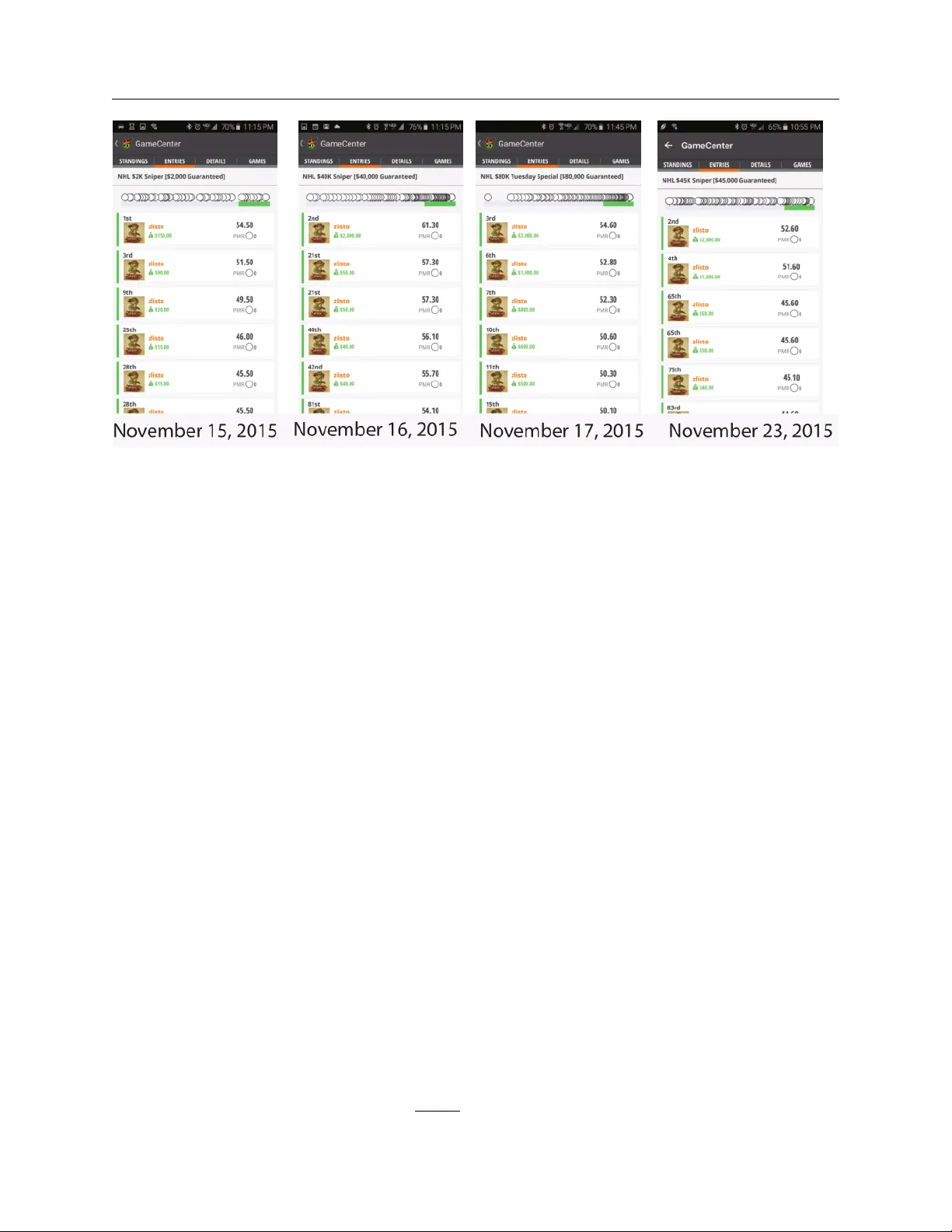
Submitted to INFORMS J ournal on Optimization manuscript A uthors ar e encouraged to submit new papers to INFORMS jour nals by means of a style ﬁle template, which includes the journal title. Howev er , use of a template does not certify that the paper has been accepted for publication in the named journal. INFORMS journal templates are for the exclusive purpose of submitting to an INFORMS jour nal and should not be used to distribute the papers in print or online or to submit the papers to another publication. Picking W inners in Daily F antasy Sports Using Integer Programming David Scott Hunter Operations Research Center , Massachusetts Institute of T echnology , Cambridge, MA 02139, dshunter@mit.edu Juan Pablo V ielma Department of Operations Research, Sloan School of Management, Massachusetts Institute of T echnology , Cambridge, MA 02139, jvielma@mit.edu T auhid Zaman Department of Operations Management, Sloan School of Management, Massachusetts Institute of T echnology , Cambridge, MA 02139, zlisto@mit.edu W e consider the problem of selecting a portfolio of entries of ﬁxed cardinality for contests with top-heavy payoff structures, i.e. most of the winnings go to the top-ranked entries. This framework is general and can be used to model a variety of problems, such as movie studios selecting movies to produce, venture capital ﬁrms picking start-up companies to in vest in, or individuals selecting lineups for daily fantasy sports contests, which is the example we focus on here. W e model the portfolio selection task as a combinatorial optimization problem with a submodular objectiv e function, which is given by the probability of at least one entry winning. W e then show that this probability can be approximated using only pairwise mar ginal probabilities of the entries winning when there is a certain structure on their joint distribution. W e consider a model where the entries are jointly Gaussian random variables and present a closed form approximation to the objectiv e function. Building on this, we then consider a scenario where the entries are giv en by sums of constrained resources and present an integer programming formulation to construct the entries. Our formulation uses principles based on our theoretical analysis to construct entries: we maximize the expected score of an entry subject to a lower bound on its variance and an upper bound on its correlation with previously constructed entries. T o demonstrate the effecti veness of our integer programming approach, we apply it to daily fantasy sports contests that have top-heavy payoff structures. W e ﬁnd that our approach performs well in practice. Using our inte ger programming approach, we are able to rank in the top-ten multiple times in hockey and baseball contests with thousands of competing entries. Our approach can easily be extended to other problems with constrained resources and a top-hea vy payoff structure. K ey wor ds : combinatorial optimization, statistics, integer programming, sports analytics History : 1 Hunter , Vielma, and Zaman: Picking W inners in Daily F antasy Sports Using Integer Pr ogramming 2 Article submitted to INFORMS Journal on Optimization ; manuscript no. 1. Introduction Imagine one must select a portfolio of entries for a contest where all or nearly all of the winnings go to the top performing entry . Because of the top-heavy payof f structure, one natural strategy is to select the entries in such a way that maximizes the probability that at least one of them has exceptional performance and wins the contest. W e refer to this as the picking winners problem. In Hunter and Zaman (2017) the picking winners problem is introduced, and this study illustrates how this frame work can be used to model the challenge faced by a venture capital fund. In particular, a venture capital fund will in vest in a portfolio of start up companies and due to the top-hea vy return structure, if one of the companies becomes a huge success, the fund will earn a lar ge return. The picking winners frame work can be also be used to model a wide variety of other problems that hav e top-heavy payoff structure. For instance, pharmaceutical compa- nies want to select a set of drugs to in vest research resources in such that the probability at least one of the drugs is a major success is maximized. F or another e xample, consider a movie studio that has to select a set of movies to produce, and the movie studio achieves success if one of the movies is a blockbuster hit. This frame work can also model daily fantasy sports contests where people enter lineups of players in a sport (such as hockey or baseball) into daily contests where the top scoring entry wins a huge amount of money . All of these examples require one to select a set of entries (drugs, start-up companies, movies, lineups of players) to maximize the probability that at least one of them has exceptional performance and wins. Many applications of the picking winners framework require one to select entries from a ﬁxed set, such as start-up companies for v enture capital funds. Howe ver , there are also scenarios where the set of entries is not provided in adv ance. Instead, the entries must be constructed from a set of constrained resources. One example of this is daily fantasy sports contests, where one must select players for a lineup, but the players must satisfy b udget and position constraints imposed by the company running the contests. F or instance, in hocke y contests, a lineup can only hav e one goalie. In these types of situations one must develop a method to construct the entries in a manner that respects the constraints b ut still maximizes the probability of winning. T o select the entries one requires some predictiv e model of ho w well the entries will perform. Howe ver , this information alone will not be sufﬁcient to select a good set of entries. The goal is to maximize the probability that at least one entry wins. One may select entries that have a high probability of indi vidually winning. Howe ver , if these entries have a high positiv e correlation, then the probability that at least one of them wins may not be as large as for a set of entries with slightly lower winning probabilities, but lower correlation so they cover more possible outcomes. Therefore, choosing a good set of entries would require information on their joint distribution in addition to their marginal probabilities of winning. Intuitiv ely , a good set of entries will each hav e a high probability of winning, but also not be too positiv ely correlated in order to div ersify the set of entries. What one needs to do is understand the trade-off between the winning probability of the entries and their correlations in order to select a good set of entries. Hunter , Vielma, and Zaman: Picking W inners in Daily F antasy Sports Using Integer Pr ogramming Article submitted to INFORMS Journal on Optimization ; manuscript no. 3 In Hunter and Zaman (2017) it was shown that the general picking winners problem is NP-hard. Nev- ertheless, it has a non-ne gativ e, non-decreasing, and submodular objectiv e function, which implies that a greedy solution has strong performance guarantees. Naturally then, these results motiv ate using a greedy approach to solve the picking winners problem. Ho wever , Hunter and Zaman (2017) focuses on the sce- nario where at each iteration of the greedy approach one simply chooses the entry (for instance, a start-up company) from a particular ground set that maximizes the marginal gain in the objectiv e function. In this study , we will focus on the situation where the entries must be constructed from constrained resources and cannot simply be chosen from a ground set. Our problem is closely related to the problem of maximizing a stochastic monotone submodular function with respect to a matroid constraint (Asadpour and Nazerzadeh 2015). Howe ver in our case the objective function is the probability of at least one entry winning, which many times lacks a closed form e xpression. Therefore, we cannot e ven e valuate the objecti ve function for a set of entries, which will pre vent us from directly applying the greedy approach. T o overcome these challenges, we dev elop a greedy approach for constructing entries from constrained resources for top-heavy contests, where at each step in the greedy approach we solve an integer program- ming problem. Our approach is fairly general and can be applied to a variety of problems. T o demonstrate the effecti veness of our approach, we use it to construct entries for daily fantasy sports competitions. W e were able to perform exceptionally well in these contests across multiple sports. T o provide more context for our results, we next present a brief o vervie w of the structure of daily fantasy sports contests. 1.1. Daily F antasy Sports Contests Daily fantasy sports have recently become a huge industry . For instance, DraftKings, the leading company in this area, reported $30 million in rev enues and $304 million in entry fees in 2014 (Heitner 2015). While there is an ongoing legal debate as to whether or not daily fantasy sports contests are gambling (Board 2015, Easton and Newell, Getty et al. 2018), there is a strong element of skill required to continuously win contests as e videnced by the fact that the top-one percent of players pay 40 percent of the entry fees and gain 91 percent of the proﬁts (Harwell 2015). This space is competiti ve, with many users employing advanced analytics to pick winning lineups. Several sites such as Rotogrinders hav e been created that solely focus on daily fantasy sports analytics (Rotogrinders 2015). Other sites such as Daily Fantasy Nerd ev en offer to provide optimized contest lineups for a fee (DailyF antasyNerd 2015). There are a variety of contests in daily fantasy sports with different payoff structures. Some contests distribute all the entry fees equally among all lineups that score abov e the median score of the contest. These are known as double-up or 50/50 contests. They are relativ ely easy to win, but do not pay out much. Other contests giv e a disproportionately high fraction of the entry fees to the top scoring lineups. W e refer to these as top-heavy contests. W inning a top-heavy contest is much more difﬁcult than winning a double- up or a 50/50 contest, but the payoff is also much greater . T ypical entry fees range from $3 to $30, while Hunter , Vielma, and Zaman: Picking W inners in Daily F antasy Sports Using Integer Pr ogramming 4 Article submitted to INFORMS Journal on Optimization ; manuscript no. the potential winnings range from thousands to a million dollars (DraftKings 2015). These contests occur nearly ev ery day, providing multiple opportunities to test and ev aluate dif ferent strategies. For these reasons, daily fantasy sports pro vide a great opportunity for us to test our approach to picking winners. The entry to a daily fantasy sports contest is called a lineup, and it consists of a set of players in the giv en sport. An added complication is the fact that there are constraints on the players used to build a lineup. A daily fantasy sports company sets a price (in virtual dollars) for each player in a sport. These prices vary day-to-day and are based upon past and predicted performance (Steinberg 2015). Lineups must then be constructed within a ﬁxed b udget. For instance, in DraftKings hockey contests, there is a $50,000 budget for each lineup. There are further constraints on the maximum number of each type of player allowed and the number of different teams represented in a lineup. Finding an optimal lineup is challenging because the performance of each player is unknown and there are hundreds of players to choose from. Howe ver , predictions for player points can be found on a host of sites such as Rotogrinders (Rotogrinders 2015) or Daily F antasy Nerd (DailyF antasyNerd 2015) that are fairly accurate, and man y fantasy sports players have a good sense about ho w players will perform. This suggests that the main challenge is not in predicting player performance, but in using predictions and other information to construct the lineups. There ha ve been man y pre vious studies on ho w mathematical optimization and analytical methods can be used to assist sporting or ganizations. F or instance, Sharp et al. (2011) use integer programming to construct Cricket teams, Pantuso (2017) propose an optimization model to maximize the expected value of a Euro- pean football club, ¨ Ozl ¨ u and Sokol (2016) employ integer programming to solve the problem of assigning and scheduling minor league scouts for Major League Baseball teams, and Sokol (2003) generate optimal baseball batting orders that are robust under uncertainty in skill measurement. Additionally , there have been many studies that ha ve applied analytical methods to in consumer sporting competitions. For instance, mul- tiple studies ha ve considered the problem of predicting the maximum number of winners in the National Collegiate Athletic Association (NCAA) March Madness college bask etball tournament (Brown and Sok ol 2010, Guestrin et al. 2005, Kaplan and Garstka 2001, Kvam and Sokol 2006). There has also been work that considers ranking NCAA Football teams (K olbush and Sokol 2017). In addition to these studies, there has been pre vious research on the topic of season-long fantasy sports. For instance, in Becker and Sun (2016) the authors present a mix ed integer program that optimizes draft selection and weekly lineup selection for fantasy football. Fry et al. (2007) present a dynamic programming approach for fantasy football draft selection. Ber gman and Imbrogno (2017) use optimization tools for National Football League surviv or fantasy pools. All of these studies illustrate that optimization can be a useful tool in fantasy sports. Howe ver , all of these studies focus on season-long fantasy contests, which do not necessarily coincide with the problem of picking winners in daily fantasy contests that we study in this work. Hunter , Vielma, and Zaman: Picking W inners in Daily F antasy Sports Using Integer Pr ogramming Article submitted to INFORMS Journal on Optimization ; manuscript no. 5 In a recent study a stochastic integer programming approach is proposed to construct lineups for daily fantasy sports contests that maximizes the expected payout (Newell and Easton 2017). In this study , the author’ s assume that each athlete’ s fantasy points and independent. Using their approach they are able to maximize the probability of achie ving a payout, but they do not ﬁnd success in real DraftKings contests. W e take a dif ferent approach to this problem, and with our approach we are able to win several DraftKings contests. Achieving this required real entries in the contests that generated winnings of up to thousands of dollars per entry (See Figure 1). T o av oid any related ethical or conﬂict of interest issues, we donated all winnings generated during this study (around $15,000) to the Greater Boston Food Bank, which is a non-proﬁt hunger-relief or ganization in eastern Massachusetts. 1.2. Our Contributions Integer programming is a natural tool to use to construct entries because of the different constraints. The challenge comes in understanding how to formulate the integer program to maximize the probability of winning. In this work we present a sequential integer programming approach that attempts to do this. W e begin by ﬁnding a tractable approximation for the objectiv e function (the probability of winning), and sho w that the error of this approximation is small when the underlying distribution of the entries satisﬁes certain natural properties. From this approximation we are able to extract a set of heuristic principles for constructing entries. First, the entries’ scores should hav e a large expected value and variance. This increases the mar ginal probability of an entry winning. Second, the entries should also ha ve lo w correlation with each other to make sure they cov er a large number of possible outcomes. These principles form the foundation of our integer programming approach that sequentially constructs entries with maximal mean subject to constraints on their v ariance and correlation with previously constructed lineups. W e apply our approach to top-heavy hocke y and baseball contests in DraftKings. The contests we focus on had thousands of entrants and top payouts of se veral thousand dollars. The entries that we construct with our inte ger programming approach are able to rank in the top ten in these contests multiple times, as sho wn in Figure 1. This is a non-tri vial achiev ement gi ven the large size of the contests. One may be concerned that our integer programming approach is a betting tool that constitutes cheating. Howe ver , daily fantasy sports hav e been shown to be games of skill (Getty et al. 2018), so the use of such tools is considered fair game and are routinely of fered as a for-proﬁt service (DailyFantasyNerd 2015, Rotogrinders 2015). Our hope is that by making our results and code here public, we can help to ele vate the lev el of the players that compete by introducing them to advanced operations research and management science techniques, which they could then apply elsewhere. Nonetheless, as mentioned before, all winnings were donated to charity to av oid any conﬂict of interest issues. Pre vious studies (Kvam and Sokol 2004, Sokol 2004) hav e found that sports can be used as a valuable tool to teach students analytical tools. Our success in using integer programming in daily fantasy sports Hunter , Vielma, and Zaman: Picking W inners in Daily F antasy Sports Using Integer Pr ogramming 6 Article submitted to INFORMS Journal on Optimization ; manuscript no. has also exposed a whole new audience to analytics and optimization. W e hav e presented our results at the Sloan Sports Analytics Conference in 2016 and 2017 (Hunter et al. 2016, Zaman 2017b), giving a non- technical audience a tutorial on integer programming via daily fantasy sports. W e hav e also presented our work in multiple analytics classes for under graduate, graduate and MB A students at MIT and Harv ard. Our optimization code is av ailable on GitHub (Hunter 2016, Zaman 2017a). Daily fantasy sports have proved itself to be an excellent application to get ne w people interested in studying analytics and optimization. In particular , graduate students at MIT routinely present e xtensions of this work to other sports as part of their class projects. W e strongly believ e that a crucial aspect for the past and future success of this study as an educational tool to disseminate the ef fectiveness of operations research and analytics tools is its relativ e simplicity . Indeed, the models and tools are intuiti ve and interpretable for anyone with a basic background in optimization. Nonetheless, these tools provided a signiﬁcant edge in an en vironment where highly technical machine learning tools are widely used by both e xperts and users that barely understand their principles. For this reason we hav e purposely av oided adding complexity for complexity’ s sake, particularly when it does not provide a practical beneﬁt. The remainder of the paper is structured as follo ws. In Section 2 we reconsider the picking winners prob- lem, and de velop an algorithm to sequentially construct each entry using an inte ger program. W e present an empirical analysis of hock ey data and de velop predicti ve models of player performance in Section 3 for use in our integer programming formulation. In Section 4 we specialize our integer programming formulation for daily fantasy sports contests, with a focus on hockey . W e e valuate the performance of our approach in actual fantasy hockey contests in Section 5. W e conclude in Section 6. All proofs, unless otherwise stated, are included in the appendix. 2. Problem F ormulation Using similar notation to Hunter and Zaman (2017), we consider a set of ev ents E = { E i } m i =1 deﬁned on a probability space (Ω , F , P ) , with sample space Ω , σ -algebra F , and probability measure P . Using this notation, each event E i corresponds to an entry i in the contest winning. The goal then is to select a subset S ⊆ [ m ] = { 1 , . . . , m } of size k such that we maximize the probability that at least one item in S wins, which is giv en by P  S i ∈S E i  . For notational con venience, we denote U ( S ) = P  S i ∈S E i  . Formally then, the picking winners problem is gi ven by the following optimization problem max S ⊆ [ m ] , |S | = k U ( S ) . (2.1) Before continuing with our analysis, we ﬁrst begin by re viewing some of the key results from Hunter and Zaman (2017) concerning the picking winners problem. For conv enience, we reproduce the proofs of Hunter , Vielma, and Zaman: Picking W inners in Daily F antasy Sports Using Integer Pr ogramming Article submitted to INFORMS Journal on Optimization ; manuscript no. 7 Figure 1 Screenshots of the performance of our top integer pr ogramming lineups in real DraftKings hocke y contests with 200 linueps entered. these results in Section 7. For notation, we will let S g be the greedy maximizer of U ( S ) and let S ∗ be the maximizer of U ( S ) . In general, solving the picking winners optimization problem can be dif ﬁcult, as sho wn by the following result. Theorem 2.1 (Hunter and Zaman (2017)) Maximizing U ( S ) is NP-har d even for discr ete uniform distri- butions. Despite the computational complexity in maximizing U ( S ) , the objectiv e function possesses some nice properties that we can use to obtain good solutions ef ﬁciently , which are gi ven by the follo wing result. Lemma 1 (Hunter and Zaman (2017)) The function U ( S ) is non-ne gative, non-decr easing and submod- ular . From Theorem 2.1, we know that the picking winners problem given by (2.1) can be dif ﬁcult. Ho wev er , the submodular property from Lemma 1 allo ws us to ﬁnd a good solution using a greedy approach where we choose the ev ents one at a time to giv e the maximal increase in the objectiv e function. For submodular functions we hav e guarantees on the sub-optimality of such greedy solutions, as the follo wing classic result sho ws. Theorem 2.2 (Nemhauser et al. (1978)) Let U ( S ) be a non-decr easing submodular function and let S g be its gr eedy maximizer . Then U ( S g ) U ( S ∗ ) ≥ 1 − e − 1 . (2.2) Hunter , Vielma, and Zaman: Picking W inners in Daily F antasy Sports Using Integer Pr ogramming 8 Article submitted to INFORMS Journal on Optimization ; manuscript no. Theorem 2.2 pro vides a strong bound for the sub-optimality of a greedy solution to the picking winners problem. In practice, a greedy solution can often be found efﬁciently , which is important as time can be a limiting factor in many applications. For these reasons, we will continue by considering a greedy approach to the picking winners problem. Ideally , a greedy solution to the picking winners problem would also be an optimal solution. In the case of all the e vents E i being independent, from Hunter and Zaman (2017) we kno w that a greedy solution is in fact optimal: Theorem 2.3 (Hunter and Zaman (2017)) F or a set of independent events E = { E 1 , . . . , E m } , let the k element gr eedy maximizer of U ( S ) be S g . Then S g is an optimal solution to the picking winners pr oblem (2.1) . This result also suggests that when the ev ents have lo w dependence, greedy solutions should perform well. In practice, the events will often hav e some dependency structure, and thus we will consider this case in more detail. 2.1. Dependent Events When the underlying e vents are dependent, solving the picking winners problem is especially dif ﬁcult. In general, a greedy solution is not an optimal solution. Additionally , with an arbitrary dependency structure between the ev ents it is often non-trivial to e ven ev aluate the objective function U ( S ) . Because of this, in this section we provide a tractable approximation to the objecti ve function when the e vents are dependent and characterize the quality of the approximation as a function of properties of the underlying distribution. W e will see that when the e vents are not too dependent upon each other , our approximation will have low error . W e start with an approximation for the objectiv e function U ( S ) . The difﬁculty of optimizing this objec- ti ve function comes from the lack of independence in the ev ents, which requires us to understand their entire joint distribution. Many times this distribution will not be av ailable to us, or if it is, ev aluating the required probability will be dif ﬁcult. T o obtain something more tractable, we deﬁne the following objecti ve function, which only utilizes pairwise correlations: U 2 ( S ) = X i ∈S P ( E i ) − 1 2 X i,j ∈S ,i 6 = j P  E i \ E j  . (2.3) This objectiv e function is obtained by expanding U ( S ) using the inclusion-exclusion principle and then only keeping terms that in volv e the intersection of two or fewer e vents. The beneﬁt of U 2 ( S ) is that it only requires us to know the probability of intersections of pairs of e vents, which is much easier to calculate than probabilities of higher order intersections. In order for this objective function to act as a good surrogate for Hunter , Vielma, and Zaman: Picking W inners in Daily F antasy Sports Using Integer Pr ogramming Article submitted to INFORMS Journal on Optimization ; manuscript no. 9 U ( S ) , we must sho w that the difference U ( S ) − U 2 ( S ) is small. If we impose certain conditions on the joint density of the e vents, we can bound this difference. T o do this we deﬁne a fe w new terms. W e assume we ha ve chosen a subset S of the entries. Let q 0 ( S ) = P ( T i ∈S E c i ) be the probability that none of the entries in S win the contest. For 1 ≤ l ≤ k , let S l be the set of all l -element subsets of S . For instance, if S = { a, b, c } then S 1 = {{ a } , { b } , { c }} and S 2 = {{ a, b } , { a, c } , { b, c }} . For an element T ∈ S l , let p 0 T = P   T i ∈ T E i  T  T j ∈S /T E c j  be the probability that all the entries in T but no other entries in S win the contest. W e then hav e the following result regarding the difference between U ( S ) and U 2 ( S ) . Theorem 2.4 Let E be a set of events on a probability space and assume |E | = m . Assume there are constants 0 < p < 1 and c > 0 such that for an y S ⊂ [ m ] with |S | = k < m , q 0 ( S ) = (1 − p ) k , kp < 1 / 2 , and for any 1 ≤ l ≤ k and T ∈ S l , p 0 T ≤ cp l . Then k p − 1 2 ( k p ) 2 ≤ U ( S ) ≤ k p and 0 ≤ U ( S ) − U 2 ( S ) ≤ 20 c ( k p ) 3 . This result shows that the error of U 2 ( S ) is approximately ( U ( S )) 3 multiplied by a constant. W e will generally be in a situation where the e vents are rare, so U ( S ) is small. Then the cubic term in the error is negligible compared to U ( S ) . The error then depends mainly on the constant c , which is related to how correlated the e vents are. W e now illustrate this with an example. Consider the case where k = 3 , and assume the marginal probability of any single ev ent occurring is 0 . 01 . If the ev ents are independent and identically distributed (i.i.d.), then q 0 ( S ) = (1 − p ) 3 = (1 − . 01) 3 , resulting in p = 0 . 01 . The condition p 0 T ≤ cp l from the theorem is satisﬁed with c = 1 . For this case, we hav e U ( S ) = 0 . 029701 and U 2 ( S ) = 0 . 029700 , resulting in an error of U ( S ) − U 2 ( S ) = 10 − 6 . From the theorem the error is upper bounded by 20 c ( k p ) 3 = 5 . 4 × 10 − 4 . No w consider the case where the three e vents are the same. This represents a situation of maximal cor- relation. W e hav e q 0 ( S ) = (1 − p ) 3 = (1 − . 01) , resulting in p = 0 . 0033 . T o satisfy the condition in the theorem, we only need to consider the set T = S , since for all other subsets T we have p 0 T = 0 . When T = S , the condition from the theorem giv es 0 . 01 ≤ c (0 . 0033) 3 . This is satisﬁed with c = 2 . 7 × 10 5 . For this case, we hav e U ( S ) = 0 . 01 and U 2 ( S ) = 0 , resulting in an error of U ( S ) − U 2 ( S ) = 0 . 01 . From the theorem the error is upper bounded by 20 c ( k p ) 3 = 5 . 4 . W e see that when the events are highly correlated, the constant c increases and the upper bound becomes loose (trivial in this case). These e xamples show that the error bound from the theorem is tighter when the e vents are not highly correlated, and the constant c is a way to capture the strength of the correlation. In the situations we consider , Hunter , Vielma, and Zaman: Picking W inners in Daily F antasy Sports Using Integer Pr ogramming 10 Article submitted to INFORMS Journal on Optimization ; manuscript no. the ev ents will hav e a low occurrence probability and will not have v ery strong correlations. Therefore, we will use U 2 ( S ) instead of U ( S ) in the remainder of this work because U 2 ( S ) is much easier to work with than U ( S ) , and it will be a good approximation to U ( S ) . 2.2. Multivariate Gaussian Random V ariables W e no w consider a probability model that captures a fairly general class of events. Let { X i } m i =1 be jointly Gaussian random v ariables with mean v ector µ and co variance matrix Σ . W e deﬁne the ev ents E i = { X i ≥ t } for some constant t . If we imagine each X i as the return of a company we in vest in, then the e vent says that company i has a return greater than t . For fantasy sports competitions, X i can be the points of lineup i and E i corresponds to the lineup exceeding t points. W e further assume that t > max 1 ≤ i ≤ m µ i because we are interested in the unlikely ev ent that one of the X i exceeds its mean by a large amount. For instance, in daily fantasy hockey contests, the maximum mean of a lineup is around 30 points, while the winning threshold t is near 60 points. W e want to choose a set of entries S ⊆ [ m ] to maximize U 2 ( S ) . T o do this, we must ﬁrst calculate the marginal and joint probabilities of the e vents. Since no closed form e xpression exists for these probabilities for multi variate Gaussian random v ariables, we instead resort to approximations. W e have the follo wing result. Theorem 2.5 Let { X i } m i =1 be jointly Gaussian random variables. Let the marginal mean and variance of X i be µ i and σ 2 i and let the correlation coefﬁcient of X i and X j be ρ ij . In addition, let z i = ( t − µ i ) /σ i . Deﬁne the function U l 2 ( S ) as U l 2 ( S ) = X i : E i ∈S 1 √ 2 π σ i ( z i + 1 /z i ) exp  − z 2 i 2  − 1 2 X i,j : E i ,E j ∈S i 6 = j 1 √ 2 π (2 t − µ 1 − µ 2 ) exp − (2 t − µ i − µ j ) 2 2  σ 2 i + σ 2 j + 2 ρ ij σ i σ j  ! . (2.4) Then U 2 ( S ) ≥ U l 2 ( S ) . The function U l 2 ( S ) is a lo wer bound on U 2 ( S ) and has a closed form expression. W e use this function to gain insights on good entries. From the expression for U l 2 ( S ) we observe some important features that characterize a subset S that will hav e a high chance of winning. W e assume that z i ≥ 1 ,, which can be done by having t be large enough. In this case, the contribution of the ﬁrst summation to U l 2 ( S ) increases for large µ i and large σ i . The contrib ution of the second summation increases for small ρ ij . There is an intuiti ve explanation for how µ i , σ i , and ρ ij impact the objecti ve function. First, the means of the chosen entries should be large so that there is a greater probability that they exceed t . Second, the variance of the entries should be large as well. This is less obvious, but the intuition here is that all one cares about is Hunter , Vielma, and Zaman: Picking W inners in Daily F antasy Sports Using Integer Pr ogramming Article submitted to INFORMS Journal on Optimization ; manuscript no. 11 having some entry’ s score e xceed t . If entries with lar ge v ariances are chosen, this increases the probability of exceeding t . While this also increases the probability that some of the entries will ha ve a low value, this is not a concern as the goal is to hav e at least one e xceed t . Third, the correlation between each pair of entries should be small. What this does is diversify the selected entries so there is a better chance that one of them exceeds t . In short, one would like S to consist of entries with high means and high variance that hav e low correlation with each other . 2.3. Picking Winners with Constrained Resour ces W e now consider a case where entries are constructed from a set of resources { Y j } p j =1 that are jointly Gaussian random variables. W e deﬁne the mean and standard deviation of Y j as µ 0 j and σ 0 j , respecti vely . W e deﬁne the correlation coef ﬁcient of Y j and Y l as ρ 0 j l . Each entry is giv en by the sum of n resources. Let us deﬁne x ij as variables that are one if resource j is in entry i and zero otherwise. Then we can write X i = P p j =1 Y j x ij . W e assume that there are certain constraints on the resources such that not e very possible subset of q resources is a feasible entry . In this scenario, we want to construct k feasible entries from the gi ven resources to maximize the probability of winning. T o do this we will develop an inte ger programming formulation that builds upon the intuitions gained in Section 2.2. Speciﬁcally , our general paradigm for the formulation will make use of the follo wing three insights. 1. Each entry has a high mean in order to increase the probability it exceeds the threshold t . 2. Each entry has a high variance in order to increase the probability it exceeds the threshold t . 3. Each pair of entries ha ve minimal correlation to increase the probability that at least one of the entries exceeds the threshold t . W e can write the mean of X i as µ i = p X j =1 µ 0 j x ij . (2.5) The v ariance of X i is σ 2 i = p X j =1 ( σ 0 j ) 2 x ij + p X j =1 p X l =1 ,l 6 = j ρ 0 j l σ 0 j σ 0 l x ij x il , (2.6) and the cov ariance of X i and X q is Cov ( X i , X q ) = p X j =1 ( σ 0 j ) 2 x ij x q j + p X j =1 p X l =1 ,l 6 = j ρ 0 j l σ 0 j σ 0 l x ij x q l , (2.7) W ith these expressions we want to understand how to construct a set of entries that will hav e a high probability of winning. T o achiev e a high mean, each entry should be chosen to maximize the sum of its resources’ means. This insight is fairly obvious and natural. The more interesting insights come from the v ariances and co variances of the entries. T o obtain a more intuitive understanding of what entries have good Hunter , Vielma, and Zaman: Picking W inners in Daily F antasy Sports Using Integer Pr ogramming 12 Article submitted to INFORMS Journal on Optimization ; manuscript no. properties with respect to their variance and cov ariance, suppose the variance of each resource is equal to one, and the correlation coefﬁcient to be either zero, δ , or − δ for some δ > 0 . W e can then characterize the v ariance of an entry by the number of pairs of resources that ha ve a positi ve or ne gativ e correlation, and the cov ariance of a pair of entries by the number of their shared resources and the number of pairs of resources with positi ve and negati ve correlations. Let us deﬁne for X i the number of positi vely and negati vely pairs of correlated resources as n + i and n − i . Let us also deﬁne for X i and X q the number of positi vely and ne gativ ely pairs of correlated resources as n + iq and n − iq , and the number of shared resources as n iq . W e will also refer to n iq as the o verlap of entries X i and X j because this is the number of resources the y hav e in common. W ith this notation, the v ariances and covariances can be written as σ 2 i = n + δ  n + i − n − i  (2.8) Cov ( X i , X q ) = n iq + δ  n + iq − n − iq  (2.9) From these expressions we gain some useful insights concerning the variances and covariances. A high v ariance can be achie ved if the entry has a lar ge n + i and a small n − i . That is, the entry’ s resources should be chosen so many of them are positiv ely correlated, and few of them are negati vely correlated. By av oiding negati ve correlations, we are making it more likely that either the resources all have a high value or all ha ve a low v alue. The cov ariance of a pair of entries can be reduced in two ways. First, reduce the ov erlap n iq . If the entries share fewer resources, they will clearly be less correlated. Second, increase the number of pairs of resources between the lineups that ha ve a negati ve correlation, and decrease the number of pairs of resources with positi ve correlation. Limiting the number of positi vely correlated resources between lineups reduces their cov ariance and subsequent correlation coefﬁcient. 2.4. Sequential Integer Programming A pproach with Constrained Resour ces Constructing a set of entries that optimizes the U l 2 ( S ) is non-tri vial. The function is non-linear and non- con ve x. Therefore, we will not directly maximize U l 2 ( S ) . Instead, we will use the three properties discussed about U l 2 ( S ) to guide the dev elopment of a sequential integer programming approach for constructing a set of entries from constrained resources that hav e a high probability of winning. W e choose a greedy approach for three important reasons. First, from the submodular property of the original objecti ve function we have a lower bound on the performance of a greedy solution. The objective function we will use in our integer programming formulation is different from the original objecti ve function, b ut shares some of its ke y properties, so we assume the loss in optimality with our greedy approach will not be signiﬁcant. Second, the integer programming approach we propose is linear and can be solv ed quickly , which will be important in applications we consider later . Third, and most importantly , we will sho w in Section 5 that this approach performs well on actual data. In particular , we will see that with this approach we are able to consistently perform well in daily fantasy sports contests. Hunter , Vielma, and Zaman: Picking W inners in Daily F antasy Sports Using Integer Pr ogramming Article submitted to INFORMS Journal on Optimization ; manuscript no. 13 W e consider the situation described in Section 2.3 where we want to construct k entries consisting of n resources each from a set of p resources. As pre viously stated, our decision v ariable is x ij , which is 1 if resource j is in entry i . Let  x ∗ ij  p j =1 correspond to the i th greedy entry . This is the solution to our integer program in the i th iteration. W e will construct the entries sequentially in the following manner . W e choose a set of positive constants {  i } k i =1 and { γ iq } k i,q =1 . Assume we have obtained the ﬁrst i − 1 entries. W e then construct the i th entry to maximize its mean subject to its variance being larger than  i , and its cov ariance with entry q being less than γ iq for q = 1 , . . . , i − 1 . F or i = 2 , . . . , k , our inte ger program for the i th entry is maximize x p X j =1 µ 0 j x ij subject to p X j =1 ( σ 0 j ) 2 x ij + p X j =1 p X l =1 ,l 6 = j ρ 0 j l σ 0 j σ 0 l x ij x il ≥  i p X j =1 ( σ 0 j ) 2 x ij x ∗ q k + p X j =1 p X l =1 ,l 6 = j ρ 0 j l σ 0 j σ 0 l x ij x ∗ q l ≤ γ iq , q = 1 , . . . , i − 1 p X j =1 x ij = n x ∈ G . (2.10) where G ⊂ { 0 , 1 } p is some general feasible region. For constructing the ﬁrst entry we solve the integer program (2.10), but we omit the co variance constraint from the problem. The greedy approach only constrains the covariance of a lineup with the previous lineups, whereas a non- greedy approach would limit all pairwise cov ariances. By only constraining the co variance with previous lineups, the number of cov ariance constraints is linear in the number of previous entries. The variance constraints are non-linear in this formulation. W e can introduce auxiliary v ariables to make this formulation linear as is standard in many integer programming formulations. Ho wever , we take a dif ferent approach when we apply this approach to fantasy sports contests in Section 4. W e will make certain assumptions on the underlying distribution of the resources, which allo w us to makes these constraints linear . W e will see that this allo ws the integer program to be solved quickly, and it still performs well in real applications. Our approach giv es one the ﬂe xibility to choose the parameters  i and γ iq . W e may w ant the ﬁrst fe w entries’ cov ariances to be lower in order to force exploration of the space of entries, while for later entries this constraint can be relaxed to av oid excluding entries with large means. Howe ver , we will see that using a single value for γ iq and for  i works well in practice. In addition, we will also see that the choice of the v alue for γ iq depends upon the size of the space of resources. 3. Hockey Data Analysis T o demonstrate the ef fectiv eness of our approach for picking winners, we apply it to top-heavy daily f antasy sports hocke y contests as described in Section 1. The entries into these contests are known as lineups, and Hunter , Vielma, and Zaman: Picking W inners in Daily F antasy Sports Using Integer Pr ogramming 14 Article submitted to INFORMS Journal on Optimization ; manuscript no. Goalie Center Winger Defenseman Skaters 0 0.5 1 1.5 2 2.5 3 3.5 Mean Absolute Error [FPPG] Daily Fantasy Nerd Rotogrinders Goalie Center Winger Defenseman 0 1 2 3 4 5 6 7 8 Average FPPG Standard Deviation FPPG Average Player Cost [$ thousands] Winger Center 0 0.5 1 1.5 2 2.5 3 3.5 4 4.5 5 Line 1 Line 2 Line 3 Line 4 Power Play Line 1 Power Play Line 2 Average FPPG Figure 2 (top left) Mean and standard de viation of fantasy points per game (FPPG) and average player cost in DraftKings for eac h hockey position. (bottom left) Mean absolute err or of NHL player FPPG predictions of Daily F antasy Nerd and Rotogrinders f or each hocke y position. (top right) Mean FFPG of forwards in different types of lines. (bottom right) Screenhsot of an NHL lineup from DraftKings. these lineups consist of resources that are players in the National Hocke y League (NHL), which is the main hocke y league in North America. The daily fantasy contests we focus on are from the site DraftKings. W e begin by describing the basic elements of hockey and hocke y daily fantasy sports contests. T o apply our approach, we need to kno w the mean and correlation of the resources, which are the hock ey players. In this section we present models and analysis for these inputs. Section 3.2 presents predictive models for players points using publicly av ailable data, and Section 3.3 studies the structural correlations between hockey players. While our analysis focuses on DraftKings, we note that other daily f antasy sports sites hav e similar contests and point scoring systems. All data in this section was collected between October 21, 2015 and December 31, 2015. 3.1. Hockey Basics A hocke y team consists of six players: one center , two wingers, tw o defensemen, and a goalie. The centers, wingers, and defensemen are kno wn as skaters because they are free to skate on the ice rink, whereas the goalie primarily stays in front of the goal. In hocke y the aim is for a team to shoot a puck into the goal of the opposing team and the goalie’ s task is to protect the goal from any opponent scores. Hunter , Vielma, and Zaman: Picking W inners in Daily F antasy Sports Using Integer Pr ogramming Article submitted to INFORMS Journal on Optimization ; manuscript no. 15 Score type Points Goal 3 Assist 2 Shot on Goal 0.5 Blocked Shot 0.5 Short Handed Point Bonus (Goal/Assist) 1 Shootout Goal 0.2 Hat T rick Bonus 1.5 W in (goalie only) 3 Sav e (goalie only) 0.2 Goal allo wed (goalie only) -1 Shutout Bonus (goalie only) 2 T able 1 P oints system for NHL contests in DraftKings. In daily fantasy sports hockey contests there are constraints on the types of players that must be present in a lineup. For DraftKings, each lineup must consist of two centers, three wingers, two defensemen, one goalie, and one utility player that is any skater , resulting in a lineup of nine players. W e show a screenshot of one possible DraftKings lineup in Figure 2. The ﬁgure also sho ws a column labeled FPPG, which stands for fantasy points per game. This is the av erage number of fantasy points per game the player has earned throughout the current NHL season. DraftKings provides this information to help users construct their lineups. The total fantasy points for a lineup is the sum of each player’ s fantasy points. The lineup shown has 34.4 fantasy points per game. This score is in the typical range of NHL lineups in DraftKings, and it gi ves a sense of the value of different scoring actions. In a daily fantasy sports contest, there are man y ways for players to score fantasy points. Because we test our approach in DraftKings, we will focus on its points scoring system. W e summarize the details of the DraftKings scoring system in T able 1. In Figure 2 we show the basic statistics of points per game for each position av eraged ov er all NHL players. W e also show the av erage DraftKings cost per player in the ﬁgure. As can be seen, on a verage goalies tend to score almost twice as many points as all other players, and also cost twice as much. Additionally , the standard deviation of each position’ s points per game is roughly the same size as the average v alue. The centers and wingers are kno wn as forwards. In the NHL each hocke y team plays its forwards in ﬁx ed sets kno wn as lines . This means that if one player from the line, such as the center , is on the ice, then so are the other two players from the line. Each team has four standard lines and two po wer play lines, which only play when there is a po wer play as a result of a penalty . W e sho w the average points per game for players based upon their line in Figure 2. The rank of the line typically suggests how well it performs. As can be seen, line one is generally the highest scoring line. The points system of DraftKings is similar to most daily fantasy hockey points systems. It giv es more points for players that perform better , but it also has some important properties that we use to construct our lineups. The ﬁrst property concerns assists, which is passing the puck to a player who either scores or who passes the puck to the player that scores. Each assist is worth two points, and DraftKings a wards points Hunter , Vielma, and Zaman: Picking W inners in Daily F antasy Sports Using Integer Pr ogramming 16 Article submitted to INFORMS Journal on Optimization ; manuscript no. for up to two assists per goal. This is an important aspect of the scoring system because it means that for each goal scored, it is possible for a single lineup to receiv e sev en points (three points for the goal, and four points for the two assists that led to the goal). Howe ver , such a situation can only occur if all players in volv ed are on a single lineup. This suggests that to score many points, a lineup should contain all players from a single line. By putting all players from a single line in a lineup, we are essentially increasing the v ariance of the lineup. This is a popular fantasy sports tactic known as stacking . Man y expert daily fantasy sports players use stacking to win in a variety of sports contests (Bales 2015a,b, Dre wby 2015). The second property of the points system concerns goalies. If a goalie’ s team wins the game, an additional three points is awarded to the goalie. This is important because as we will see, it is possible to predict who will win an NHL hockey game with relativ ely good accuracy , so by choosing goalies on winning teams, an extra three points can be obtained, which is a signiﬁcant amount in hocke y contests gi ven that lineups a verage between 30 to 40 points. 3.2. Player P oint Predictions Many fantasy sports players dev ote a substantial amount of effort in developing elaborate prediction mod- els for players’ performance. Their advantage comes mainly from the power of their predictiv e models. Ho wever , we do not hav e the domain kno wledge required to improve upon the prediction models of the top fantasy players. Therefore, we take a dif ferent approach. Publicly av ailable player point predictions are provided by the websites Rotogrinders (Rotogrinders 2015) and Daily Fantasy Nerd (DailyFantasyNerd 2015). W e ﬁnd the predictions from these sites to be relati vely accurate, but the accuracy v aries by position. W e plot in Figure 2 the mean absolute error in points of the two sites’ predictions for different hockey positions using our data from the 2015 NHL season. W e obtain each of our predictions from Rotogrinders and Daily Fantasy Nerd roughly thirty minutes before the corresponding DraftKings contest be gan. W e see that the prediction errors of both sites are similar . Therefore, it does not seem that either one has a superior prediction model. W e b uild a predictive model for the f antasy points for each player in the NHL using these prediction sites. For a player k , let f k 1 and f k 2 be the predictions by Rotogrinders and Daily F antasy Nerd, respecti vely . For skaters, we perform a linear re gression on the player’ s points using these predictions as features. W e denote µ k as the predicted points of player k using our model. For skater k our prediction is µ k = β 0 + β 1 f 1 k + β 2 f 2 k +  k (3.1) where  k is a Gaussian error term. For goalies, we must also factor in the outcome of the game since there is a three point bonus for victory . Daily Fantasy Nerd pro vides win probabilities for each goalie, and we hav e found these estimates to be relati vely accurate. W e perform a linear regression on the goalie points using Hunter , Vielma, and Zaman: Picking W inners in Daily F antasy Sports Using Integer Pr ogramming Article submitted to INFORMS Journal on Optimization ; manuscript no. 17 (1) (2) (3) (4) (5) (6) Skater points Goalie points Goalie points Goalie points Goalie points Goalie points β 1 0.634 ∗∗∗ 0.628 ∗∗∗ 0.203 0.203 (Rotogrinders) (0.0203) (0.0864) (0.144) (0.144) β 2 0.282 ∗∗∗ -0.0173 -0.0309 -0.0301 (Daily Fantasy Nerd) (0.0242) (0.106) (0.113) (0.113) β 3 4.310 ∗ 5.304 ∗∗ 4.176 ∗ 5.172 ∗∗ (W in probability) (2.123) (2.005) (2.064) (1.941) β 0 1.334 1.686 (0.0314) (0.549) (1.032) (1.003) (1.013) (0.983) R 2 0.238 0.0858 0.0179 0.0140 0.0178 0.0139 Samples 10825 565 506 506 506 506 Standard errors in parentheses ∗ p < 0 . 05 , ∗∗ p < 0 . 01 , ∗∗∗ p < 0 . 001 T able 2 Regression coefﬁcients, R squared, and sample count for diff erent prediction models of skater and goalie points. as predictor v ariables the predictions of Rotogrinders, Daily Fantasy Nerd, and the win probability of the goalie’ s team. For a goalie k , let this win probability by p k . Then the prediction for goalie k is µ k = β 0 + β 1 f 1 k + β 2 f 2 k + β 3 p k +  k (3.2) where  k is a Gaussian error term. W e compare dif ferent prediction models in T able 2. For skaters, both Rotogrinders and Daily F antasy Nerd predictions are signiﬁcant. F or goalies, something different occurs. When we do not include the win probability we ﬁnd that only Rotogrinders is signiﬁcant. When the win probability is included, it is the only signiﬁcant feature. From T able 2 we see that the models do not hav e high accurac y . Ho wev er , our metric of interest is not accurac y , but performance in real hocke y contests. W e will test these dif ferent models in these contests in Section 5. 3.3. Player Corr elations T o create high variance lineups we must ﬁrst understand the correlations between players. There are two important correlations we look at. The ﬁrst concerns players in lines. The second concerns forwards and goalies. W e ﬁrst begin by examining the correlations of FPPG between players in the same line versus those in dif ferent lines. W e calculate the Pearson correlation coefﬁcient between the FPPG for ev ery pair of NHL forwards (centers and wingers) in the same line, and on the same team but different line. W e plot the resulting av erage correlation coef ﬁcients for each group in Figure 3. W e see that the players on the same line hav e a much higher correlation than players on different lines. This is not surprising gi ven the way fantasy points are aw arded. This correlation is most likely due to the assist/goal combinations that giv e Hunter , Vielma, and Zaman: Picking W inners in Daily F antasy Sports Using Integer Pr ogramming 18 Article submitted to INFORMS Journal on Optimization ; manuscript no. Line 1 Line 2 Line 3 Line 4 Different Line −0.2 −0.15 −0.1 −0.05 0 0.05 0.1 0.15 0.2 0.25 0.3 Corr. Coef. of Offensive Player FPPG Same Team Different Team -0.2 -0.15 -0.1 -0.05 0 0.05 0.1 0.15 0.2 0.25 0.3 Corr. Coeff. of Goalie-Skater FPPG Offensive Skater Defensemen Figure 3 (left) A verage correlation coefﬁcient of FPPG for forwar ds in the same and different lines. (right) A verage correlation coefﬁcient of FPPG for goalies and skaters in the same and opposing teams. points to multiple players who are simultaneously on the ice. This correlation should be included in a lineup to increase the v ariance. W e next look at the correlation between goalies and skaters in the same game. W e consider the correlation of FPPG for forwards and defensemen with goalies on the same and opposing team in a game. W e plot the resulting av erage Pearson correlation coefﬁcient of the FPPG for these groups in Figure 3. W e ﬁnd that the correlation is negati ve for goalies and skaters on opposing teams. For the same team the correlation is near zero. The negati ve correlation is due to the fact that if a skater scores fantasy points, it is typically because a goal was scored, which gi ves negati ve fantasy points to the goalie. On the same team the only structural condition that would correlate skaters and goalies is the win bonus and points for scoring goals. Ho wev er, this is much weaker than the neg ative correlation of goalies opposing skaters. The negati ve correlation is something we want to av oid within a lineup as it would reduce the overall v ariance. Therefore, to increase lineup v ariance, we will avoid putting goalies and skaters on opposing teams in a single lineup. 4. F antasy Hockey A pproach and Integer Pr ogramming Formulations W e now present our approach for selecting multiple lineups for hockey contests. The integer program is based upon the formulation in Section 2.4. F or the mean points of a player we use our predicti ve re gression models. Due to difﬁculties in estimation, we do not explicitly use the correlations and variances of the player’ s points. Instead we assume that the players all hav e the same v ariance and that the magnitude of the cov ariance is much smaller than the v ariance. This will lead to simple constraints for the v ariance and cov ariance. W e will construct m lineups from a set of p NHL players, and we let the v ariable x ik equal one if player k is selected for lineup i , and zero otherwise. Each player k is predicted to achiev e µ k fantasy points from our predicti ve model. Hunter , Vielma, and Zaman: Picking W inners in Daily F antasy Sports Using Integer Pr ogramming Article submitted to INFORMS Journal on Optimization ; manuscript no. 19 4.1. F easibility Constraints W e begin by formulating the basic feasibility constraints of a lineup. Daily fantasy sports contests all impose a budget B constraint on a lineup. For DraftKings, this budget is B = 50 , 000 fantasy dollars. As mentioned earlier , there is also a constraint on the number of players of each type of position. F or nota- tion, we let the cost of player j be c j . There are N T NHL teams playing in a contest, and we denote the set of players on team l by T l . In addition, we denote the set of players who are centers, wingers, defenseman, and goalies by C , W , D , and G , respecti vely . The DraftKings position constraints for the i th lineup are gi ven by 2 ≤ X j ∈ C x ij ≤ 3 , 3 ≤ X j ∈ W x ij ≤ 4 , 2 ≤ X j ∈ D x ij ≤ 3 , X j ∈ G x ij = 1 , (4.1) DraftKings also requires each lineup to have players that come from at least three different NHL teams. The team constraints for lineup i are t il ≤ X k ∈ T l x ik , l = 1 , . . . , N T N T X l =1 t il ≥ 3 , t il ∈ { 0 , 1 } , l = 1 , . . . , N T . (4.2) W e put these constraints together to obtain the feasibility constraints for a lineup: p X j =1 c j x ij ≤ B , (budget constraint) p X k =1 x ij = 9 , (lineup size constraint) Equations (4.1), (position constraint) Equations (4.2), (team constraint) x ij ∈ { 0 , 1 } , j = 1 , . . . , p. (4.3) 4.2. Stacking Lineups Using Structural Correlations W e now present the integer programming constraints on the lineup variance. The constraints we use are simpler than the general form in equation (2.10). Rather than force the variance of the lineup to be larger than a lower bound, we constrain the structure of the lineup to ensure that its variance will be large. W e assume equal variance of all players, and cov ariances that are much smaller in magnitude than the variances. This allo ws us to approximate the variance of a lineup using only the number of pairs of positi vely and ne gativ ely Hunter , Vielma, and Zaman: Picking W inners in Daily F antasy Sports Using Integer Pr ogramming 20 Article submitted to INFORMS Journal on Optimization ; manuscript no. correlated players. The constraints we present next, which we refer to as different types of stacking, e xclude any ne gativ ely correlated players and try to have a lar ge number of positiv ely correlated players. Goalie Stacking. As discussed in Section 3.3, goalies are negati vely correlated with the skaters that they are opposing. Therefore, to increase the variance of a lineup, we would like to av oid having this negati ve correlation by making sure none of the lineup’ s skaters are opposing its goalie. W e will refer to this con- straint as goalie stacking . T o model this constraint in our integer programming formulation, we denote the set of skaters who are opposing goalie k by O k . For lineup i , the goalie constraint is then gi ven by: X l ∈ O j x il ≤ 6(1 − x ij ) , ∀ j ∈ G. (4.4) This constraint will force the goalie v ariable x ik to be zero if the lineup has any skater opposing goalie k . Line Stacking. Additionally , in Section 3.3 we found that players on the same line are positiv ely cor- related. Therefore, to increase the lineup variance, we would like to impose additional constraints on our formulation that will create lineups with players on the same line. W e will refer to this as line stacking . Each entry consists of eight skaters, six being offensi ve (wingers and centers), and a line consists of three of fensive skaters. The position constraints allo w a lineup to include a maximum of two lines. T o include as much positiv e correlation as possible amongst the players, we can make a lineup hav e one complete line of three players, and one partial line with at least two players. W e do this by requiring a lineup have two partial lines and one complete line. Giv en the position constraints, this will force one of the partial lines to be the same as the complete line. T o formulate the line stacking constraints, we introduce some notation. Let N L denote the total number of lines, and let L l denote the set of players on line l . W ith this notation we can formulate the constraint of having at least one complete line in lineup i as 3 v il ≤ X j ∈ L l x ij , l = 1 , . . . , N L N L X l =1 v il ≥ 1 v il ∈ { 0 , 1 } , l = 1 , . . . , N L . (4.5) Under these constraints v il is one if lineup i has all three players from line l , and zero otherwise, and we require at least one of the v il to be one. T o formulate the constraint of having at least two players from two distinct lines, we use the follo wing constraints: 2 w il ≤ X k ∈ L l x ik , l = 1 , . . . , N L N L X l =1 w il ≥ 2 w il ∈ { 0 , 1 } , l = 1 , . . . , N L . (4.6) Hunter , Vielma, and Zaman: Picking W inners in Daily F antasy Sports Using Integer Pr ogramming Article submitted to INFORMS Journal on Optimization ; manuscript no. 21 Similar to the complete line constraints, this constraint sets w il to one if at least two out of three players of line l are in lineup i , and there must be at least two w il equal to one. Defensemen Stacking. Lastly , we have found that defensemen that are on the ﬁrst power play line score substantially higher than defensemen that are not. While including the stronger defenseman may not affect the average points of the lineup, it could affect its actual points. If we force the lineup to hav e three teams, then the teammates of this defenseman will likely be included in the lineup. This produces additional pos- iti ve correlation within the lineup, which is desirable. Because the defenseman is from the ﬁrst line, when his team does well, we would expect the lineup to achie ve more points than if we had chosen a weaker defenseman. W e will refer to this as defensemen stacking . T o model this constraint, let P D denote the set of defensemen that are on any team’ s ﬁrst power play line. Then, to use only these defensemen in lineup i we add the follo wing constraints to our integer programming formulation: x ij = 0 ∀ j ∈ D \ P D . (4.7) This constraint makes sure that any defenseman that is chosen for the lineup is also in the ﬁrst power play line of some team. There are man y other constraints that could be added to the model, such as forcing a lineup to ha ve e very player on a team’ s ﬁrst power play , imposing constraints to have se ven players from one game, etc. W e did not in vestigate all the possible types of stacking, but they can all be naturally incorporated into our integer programming formulation. In this work we focus on the constraints presented because they capture the major structural correlations in hocke y . 4.3. Overlap Constraints Our integer programming formulation in Section 2.4 had a upper bound on the covariance of lineup i with the previous i − 1 lineups. W e assume that the player variance is much larger in magnitude than the player cov ariances. Using this assumption, we approximate the correlation of lineups i and j as simply the o verlap of the two lineups. W e can then add constraints to upper bound this overlap with all pre vious i − 1 lineups. W e will refer to these as overlap constraints. W e let x ∗ lj be the optimal value of the variable for player j in lineup l . W e deﬁne the overlap constraints for lineup i as p X j =1 x ∗ lj x ij ≤ γ , l = 1 , . . . , i − 1 . (4.8) These constraints make sure that lineup i will hav e no more than γ players in common with any pre viously constructed lineup. W e refer to γ as the maximum lineup overlap. Decreasing γ forces the lineups to be more di verse, whereas for larger γ the lineups may share more players. W e will see in Section 5 ho w the choice of γ is impacted by the number of NHL games being played on a gi ven night. Hunter , Vielma, and Zaman: Picking W inners in Daily F antasy Sports Using Integer Pr ogramming 22 Article submitted to INFORMS Journal on Optimization ; manuscript no. 4.4. Complete Sequential Integer Programming A pproach W e now present the complete sequential integer programming approach for constructing k lineups. W e obtain lineup i = 1 , . . . , k by solving maximize x p X j =1 µ j x ij subject to Equation (4.3) (feasibility constraints) Equation (4.8) (ov erlap constraints) Any subset of equations (4.4) , (4.5) , (4.6) , (4.7) (stacking constraints) . (4.9) By solving this integer programming formulation iterativ ely k times, each time updating the ov erlap con- straints with the previously found solutions, one obtains the k greedy lineups. This formulation allows ﬂexibility in the choice of stacking constraints, prediction model, maximum lineup overlap, and number of linueps constructed. W e will see next ho w to select the best settings using data from real fantasy hockey contests. 5. P erformance W e now ev aluate the performance of our approach on real daily fantasy sports hockey contests. T o obtain data on the performance of the population lineups in se veral actual DraftKings hocke y contests we need to enter the contests. As entrants, we are able to do wnload the lineups and points of every lineup in the contest. In total we hav e data for 38 different top-hea vy contests between October 21, 2015 and December 31, 2015, with each containing se veral thousand entrants. W e ev aluate how much proﬁt our lineups would hav e made in each contest competing against the actual population lineups. W e inv estigate a variety of settings, including the number of lineups, type of stacking, prediction model, and maximum ov erlap. W e combine the different constraints from Section 4.2 to create six different types of stacking, which are summarized in T able 3. The ﬁrst type is no stacking, which only uses the basic constraints and none of the stacking constraints. All the other types of stacking use goalie stacking (equation (4.4)) as this is a natural neg ative correlation we wish to av oid. In addition, all the other types of stacking require at least one complete line (equation (4.5)), and at least two partial lines (equation (4.6)). Only two defensemen are allo wed in T ype 2, the logic being that the utility player should be a forward that will score more points, as was seen in Figure 2. T ypes 3 and 4 use defensemen stacking (equation (4.7)). T ypes 4 and 5 require exactly three different teams to be represented on a lineup. This constraint increases the lineup variance by having more players on the same team in the lineup. 5.1. Impact of Stacking and Number of Lineups W e begin by in vestigating the performance of each type of stacking versus the number of lineups entered. W e create different numbers of lineups for each type of stacking with a maximum lineup ov erlap of seven Hunter , Vielma, and Zaman: Picking W inners in Daily F antasy Sports Using Integer Pr ogramming Article submitted to INFORMS Journal on Optimization ; manuscript no. 23 No stacking T ype 1 T ype 2 T ype 3 T ype 4 T ype 5 Equation (4.3) Equation (4.3) Equation (4.4) Equation (4.5) Equation (4.6) Equation (4.3) Equation (4.4) Equation (4.5) Equation (4.6) X j ∈ D x ij = 2 Equation (4.3) Equations (4.4) Equations (4.5) Equations (4.6) Equations (4.7) Equation (4.3) Equations (4.4) Equations (4.5) Equations (4.6) Equations (4.7) N T X k =1 t ik = 3 X k ∈ T l x ik ≤ 6 t il , l = 1 , . . . , N T Equation (4.3) Equations (4.4) Equations (4.5) Equations (4.6) N T X k =1 t ik = 3 X k ∈ T l x ik ≤ 6 t il , l = 1 , . . . , N T T able 3 Summary of the constraints for different types of stac king in our integer programming form ulation for constructing hoc key lineups. 1 lineup 100 lineups 200 lineups −100 0 100 200 300 400 500 Mean profit margin [%] No Stacking Type 1 Type 2 Type 3 Type 4 Type 5 Figure 4 Plot of the mean proﬁt mar gin in DraftKings hockey contests ver sus the number of integer programming lineups. The plots are f or different types of stacking constraints. The maxim um lineup overlap allowed is se ven. 1 lineup 100 lineups 200 lineups 0 500 1000 1500 2000 Profit margin [%] Figure 5 Bo xplot of the proﬁt margin in DraftKings hoc key contests versus the number of integer programming lineups. The lineups use T ype 4 stacking and a maxim um lineup overlap of seven. Hunter , Vielma, and Zaman: Picking W inners in Daily F antasy Sports Using Integer Pr ogramming 24 Article submitted to INFORMS Journal on Optimization ; manuscript no. and calculate the mean proﬁt margin across all contests. In calculating the mean proﬁt margin, we must adjust for the fact that when we enter more lineups, there will be some entries that cannot be in the contest pool now because of DraftKings lineup entry limits. T o adjust for this, we randomly sample lineups to delete from the historical data as we increase the number of lineups we enter , and we report our mean proﬁt mar gin across one-thousand trials of this random process. W e plot the results in Figure 4. W e observ e that the lowest proﬁt margin is achiev ed by no stacking. This shows the importance of stacking lineups to increase lineup v ariance. T ype 4 stacking achie ves the highest proﬁt margin for 100 and 200 lineups. For one lineup, T ype 3 stacking has a higher mean proﬁt margin due to a single contest where the proﬁt margin is quite large. Excluding this single outlier , T ype 4 stacking has the highest mean proﬁt margin for one lineup. Recall that T ype 4 stacking includes goalie stacking, line stacking (complete and partial), defensemen stacking, and at most three different teams. It has more stacking than all other types, which we expect to giv e its lineups more v ariance. W e see from the data that this maximizing v ariance strategy is ef fectiv e for winning top-heavy contests. It seems from Figure 4 that the mean proﬁt margin is largest for one lineup. Ho wev er, this is a decei ving statistic because the mean is dictated essentially by a single outlier for these top-hea vy contests. A more accurate picture is provided by the boxplot in Figure 5. Here we sho w the proﬁt mar gin for T ype 4 stacking with a maximum lineup overlap of seven. W e see that with one lineup, the median proﬁt margin is -100%. Ho wever , with more lineups, the median proﬁt margin becomes larger . In addition, the 75th percentile is larger for 200 lineups than for 100 lineups. Moreo ver , for 100 and 200 lineups it can be seen there are many outliers that produce much of the proﬁt, whereas with one lineup there are no outliers. This sho ws that with more lineups the distribution of the proﬁt mar gin is shifted upw ard and given a slightly f atter tail. Therefore, to win more money consistently , it is advantageous to use more lineups (at least up to the limit imposed by real-life contests). 5.2. Impact of Prediction Models W e ne xt in vestigate the impact of the different prediction models we de veloped in Section 3.2 on our perfor - mance. W e consider T ype 4 stacking, a maximum lineup ov erlap of sev en, and 200 lineups. The prediction models we consider use Rotogrinders predictions, Daily Fantasy Nerd predictions, both sites’ predictions, and both sites plus the win probability . W e show in Figure 6 the mean proﬁt margin of dif ferent prediction models for different numbers of integer programming lineups. W e see here that the model with all three features does the best or near the best for each number of lineups. The reason here may be that by including the win probability , the integer programming lineups are more biased tow ards goalies expected to win the games, resulting in a better chance of obtaining the game win bonus of three points. Ho wev er, we saw in Section 3.2 that the regression models had poor performance in terms of predicti ve accuracy . Therefore, it is not clear from our analysis which model has the clear adv antage. Hunter , Vielma, and Zaman: Picking W inners in Daily F antasy Sports Using Integer Pr ogramming Article submitted to INFORMS Journal on Optimization ; manuscript no. 25 1 lineup 100 lineups 200 lineups −50 0 50 100 150 200 Mean profit margin [%] DFN Rotogrinders DFN and Rotogrinders DFN, Rotogrinders, and Vegas odds Figure 6 Plot of the mean proﬁt mar gin of our integer programming approach in DraftKings hoc key contests with different prediction models. The models considered are Daily F antasy Nerd predictions (DFN), Rotogrinders predictions, DFN and Rotogrinder s predictions, and DFN and Rotogrinders predictions with V egas odds. The maximum lineup o verlap allowed is seven and constraint type f our is used for the integer programming lineups. <4 games 4 to 6 games 7−9 games >9 games −50 0 50 100 150 200 250 300 Mean profit margin [%] Max. overlap = 4 Max. overlap = 7 Max. overlap = 5 Max. overlap = 6 Figure 7 Plot of the mean proﬁt mar gin 200 integer programming lineups with T ype 4 stac king in DraftKings hocke y contests versus maximum lineup o verlap for different number of NHL hoc key games being play ed. 5.3. Impact of Maximum Lineup Overlap One parameter we can adjust in our model is the maximum lineup overlap. By decreasing the allowed ov erlap, we force the lineups to be more div erse. W e ﬁnd that the degree of div ersity we want depends upon ho w large the space of lineups is. The size of the lineup space on a given night is larger if there are Hunter , Vielma, and Zaman: Picking W inners in Daily F antasy Sports Using Integer Pr ogramming 26 Article submitted to INFORMS Journal on Optimization ; manuscript no. more NHL games being played. W e plot the mean proﬁt margin for 200 integer programming lineups as a function of the number of games played in a night for different v alues of the maximum lineup overlap in Figure 7. These lineups were created using T ype 4 stacking. For nights with fewer than four games, a maximum lineup overlap of sev en does best. For a larger number of games, it seems that decreasing the maximum lineup overlap improves performance. For instance, for nights with more than nine games, an ov erlap of four does best. The reason for this is that when there are few games being played, the lineup space is smaller and probably has fewer good lineups. By reducing the maximum lineup overlap, we end up not selecting these good lineups and instead choose many poor lineups. Howe ver , on nights with many games, there is a huge lineup space that has several dif ferent good lineups. A smaller maximum lineup ov erlap causes the integer program to choose sev eral of these good lineups, increasing the chance that one of them will achie ve a high rank. F or maximum lineup o verlaps smaller than four we found that it becomes dif ﬁcult to obtain 200 feasible lineups. Maximum lineup o verlaps lar ger than sev en produce lineups that are too similar and do not provide enough div ersity . Therefore, the maximum lineup overlap should be tuned between four and se ven depending on how man y games are being played on a giv en night. 5.4. Lineup Creation Order V ersus Lineup P erformance Rank In constructing our lineups, each one is constructed sequentially to create multiple lineups. One question to ask is do the lineups that are created earlier perform better? T o in vestigate this, we set the integer pro- gramming approach to create 200 lineups with T ype 4 stacking and a maximum ov erlap of sev en. W e then e valuate their performance rank relati ve to each other in the contests. This allo ws us to look at se veral statis- tics relating the creation rank and the performance rank of the lineups. W e ﬁrst in vestigate the Spearman rank correlation coefﬁcient between these two rankings. W e ﬁnd that the a verage value of the correlation coef ﬁcient across the different contests is 0.09 with a standard de viation of 0.1. This suggests that there is little correlation between the creation rank and performance rank of the lineups. T o div e deeper into the analysis, we plot in Figure 8 two different sets of data. First, we show a boxplot of the creation rank of the best performing lineup. Second, we show the performance rank of the ﬁrst created lineup. W e see that the median performance rank of the ﬁrst created lineup is 74.5. This sho ws that the ﬁrst created lineup has a slightly , but not substantially improv ed performance. For the best performing lineup, the median creation rank is 124.5. Therefore, while the ﬁrst created lineup is slightly better , the winning lineup is generally one of the later created lineups. This supports our ﬁnding of a lo w correlation between the creation and performance rank of the lineups. 5.5. Mean and Standard Deviation of Lineup P oints V ersus Proﬁt Margin One way to characterize the lineups produced by our approach is by the mean and standard deviation of their points. W e can compare these with the mean and standard de viation of the points of all lineups in a contest. Let us deﬁne the mean and standard deviation of our optimized lineups as µ 1 and σ 1 and of the population Hunter , Vielma, and Zaman: Picking W inners in Daily F antasy Sports Using Integer Pr ogramming Article submitted to INFORMS Journal on Optimization ; manuscript no. 27 0 50 100 150 200 250 Contest rank of first created lineup Creation rank of best lineup Figure 8 Plot of the performance rank of the ﬁr st created lineup and the creation rank of the best performing lineup. There were 200 integer pr ogramming lineups created with T ype 4 stacking and a maximum overlap of se ven. lineups as µ 0 and σ 0 . W e will look at the dif ference in these parameters for our lineups and the population lineups for each contest. W e use 200 integer programming lineups with T ype 4 stacking and a maximum ov erlap of se ven and plot the proﬁt mar gin v ersus the difference in the mean and standard deviation in Figure 9. One can see that there is a substantial variation in mean difference, which ranges from -10 to 20 points. When it is belo w zero, no proﬁt is made, but when it is abov e zero, a substantial proﬁt is made. This is a result of the fact that the lineups must satisfy the stacking constraints that increase their indi vidual v ariance. The result is that when the actual points are realized, we are either far above or far below the population mean. The standard de viation of the integer programming lineups is generally belo w the population standard de viation. This is because we are choosing lineups that have some correlation because they are designed to maximize points, even though the indi vidual lineups are designed to ha ve a high v ariance. From Figure 9 one can see that we are equally likely to be either above or belo w the population mean. Ho wever , because the contest payof f structure is so asymmetric, with a maximum loss of 100%, b ut a maximum g ain that is at least an order of magnitude larger , our lineups end up being proﬁtable. 5.6. Implementation and Runtime All formulations were constructed using the JuMP algebraic modeling language (Dunning et al. 2017, Lubin and Dunning 2015), which is written in the Julia programming language (Bezanson et al. 2012). This allo wed us to test the runtime of our approach for various inte ger programming solvers. The complete software used to constr uct the integer programming lineups is a vailable at an open-source GitHub webpage (Hunter 2016). In practice, we must wait for information about the goalies that are playing to be posted before we construct our lineups. Goalies do not play e very night, so if we do not wait for this information, we may put goalies in lineups who are not playing and recei ve zero points for them. This goalie information is generally Hunter , Vielma, and Zaman: Picking W inners in Daily F antasy Sports Using Integer Pr ogramming 28 Article submitted to INFORMS Journal on Optimization ; manuscript no. -20 -10 0 10 20 -4 -3 -2 -1 0 1 2 3 4 41% 1220% 114% 435% 178% 4% 102% 1445% 77% 642% 8% 13% 161% 127% 554% 744% 200 400 600 800 1000 1200 1400 σ 1 - σ 0 µ 1 - µ 0 Figure 9 Plot of proﬁt mar gin versus µ 1 − µ 0 and σ 1 − σ 0 for DraftKings hoc key contests with 200 integer programming lineups created using T ype 4 stacking and a maxim um overlap of seven. The pr oﬁt margin for each contest is indicated thr ough the color and siz e of the markers and also listed next to the marker . The × markers indicate contests where the pr oﬁt margin is not positive. posted on public websites about 30 minutes before the games begin. W e must be able to ﬁnd a solution in this time to be able to enter the contest. The ﬁrst three plots in Figure 10 sho w the time needed to solve the algorithm presented in Section 4 with T ype 4 constraints and a maximum lineup overlap of six for 100 lineups in each of our contests using different integer programming solvers. W e consider the free solvers CBC (COIN-OR 2016) and GLPK (GNU 2016) and the commercial solver Gurobi (Gurobi Optimization 2016). All computations were done using a Intel Core i5-4570 3.20GHz with 8GB of RAM. W e ﬁnd that all solvers are able to solve our algorithm for 100 lineups in under four minutes, giving sufﬁcient time to enter the lineups into the contest. While our simple formulations were more than adequate for the approach that allo wed us to consistently win over sev eral weeks, solve times could become an issue when more elaborate approaches are used. For instance, instead of solving for one lineup at a time like we propose, we could solve for two lineups at a time. T o consider lineups i and i + 1 we simply combine the i -th formulation (on variables { x ij } p j =1 ) with the i + 1 -th formulation (on v ariables { x ( i +1) j } p j =1 ) by adding a variant of the overlap constraint (4.8) which restricts the ov erlap between the two lineups and is giv en by p X j =1 x ( i +1) j x ij ≤ γ . (5.1) Unlike the original overlap constraint (4.8), constraint (5.1) is a quadratic constraint similar to the ﬁrst set of constraints of formulation (2.10). As described in Appendix 8 these constraints can be linearized through standard techniques. Howe ver , the resulting formulation can be much harder to solve. In the fourth box in Hunter , Vielma, and Zaman: Picking W inners in Daily F antasy Sports Using Integer Pr ogramming Article submitted to INFORMS Journal on Optimization ; manuscript no. 29 CBC GLPK Gurobi Gurobi: two lineups Solver 0 5 10 15 20 Runtime [minutes] Figure 10 The runtime of our algorithm for generating 100 lineups using T ype 4 constraints with an overlap parameter of 6 for 38 diff erent hockey contests with different integer pr ogramming software . The box labeled “Gurobi: tw o lineups” is the runtime when solving two lineups at a time using Gurobi. The other bo xes are f or the sequential approac h where we solve for one lineup at a time. Figure 10, we show the amount of time it takes to solv e for 100 lineups when solving lineups two at a time using Gurobi. From this plot, it is clear that solving for lineups two at a time leads to a substantial increase in runtime. W e also considered solving for two lineups at a time with the free solvers CBC and GLPK, but we found that it frequently takes longer than two hours to determine the 100 lineups. Fortunately , over 50 years of integer programming research provide plenty of opportunities to improve solve times of this and other extensions (J ¨ unger et al. 2010). In particular , we should note that our speciﬁc implementation of the Goalie Stacking constraint and the full Line Stacking constraints (i.e. (4.4) and (4.5)) are examples of what classical textbooks call weak formulations and are often associated to increased solve times. These formulations can be strengthened through standard techniques that are detailed in Appendix 8. Howe ver , no wadays such strengthening can lead to increased solve times, partly because of an increased number of constraints and partially because of the idiosyncrasies of modern solvers (Conforti et al. 2014, page 69). Indeed, for our instances this strengthened version resulted in rather signiﬁcant solve-time increments for GLPK and no noticeable improv ements for Gurobi and Cbc (See Appendix 8). Nonetheless, more advanced formulation strengthening techniques are regularly used to increase the performance of modern solv ers with very lo w implementation cost so they should not be automatically ignored (V ielma 2015). 5.7. Baseball Having demonstrated the success of our approach in hockey contests, a natural goal would be to consider ho w much our approach generalizes. T o do this, we apply our approach to top-heavy daily f antasy baseball contests in DraftKings. For baseball we only include results from May and June of 2016, so we have less Hunter , Vielma, and Zaman: Picking W inners in Daily F antasy Sports Using Integer Pr ogramming 30 Article submitted to INFORMS Journal on Optimization ; manuscript no. data for this sport than hockey . The structure of baseball contests is similar to hocke y contests. Therefore, for bre vity we will present here only a brief summary of our baseball approach and its performance on real contest data. In short, we hav e found that in our limited number of baseball contests, the method does indeed perform well and is able to place in the top ten in contests with tens of thousands of entrants multiple times. W e begin with a brief overvie w of how baseball is played and how fantasy points are scored. A baseball team consists of pitchers and hitters. The goal is for the hitters to hit the ball pitched by the opposing pitcher and then run to four bases to score runs. In fantasy sports contests a pitcher scores points for striking out batters, pitching for more innings in the game, and winning the game. A hitter scores points by hitting the pitch, scoring a run by reaching home base, or having other hitters score a run as a result of his hit, also kno wn as a run batted in or RBI. There is a great deal of similarity between the structure of hockey and baseball lineups, so we are able to almost directly use the hockey integer programming formulation with some slight modiﬁcations. W e do not go through the details of the baseball formulation here, but instead present the basic constraints. First, our objecti ve is to maximize the expected fantasy points of the lineups. Here we simply use the projections from Daily Fantasy Nerd for the expected players’ points. Second, there are feasibility constraints related to the players’ position, team, and salary . A baseball lineup consists of ten players: two pitchers and eight hitters (catcher , ﬁrst baseman, second baseman, third baseman, shortstop, and three outﬁelders). The lineup must hav e players from at least two different baseball games and the budget for a lineup is 50,000 fantasy dollars, just as in hocke y . Finally , a lineup cannot hav e more than ﬁv e hitters from one team. W e ha ve stacking and overlap constraints for baseball. As in hockey , we want to stack the baseball lineups to increase their variance. W e do this by adding constraints that remov e negati ve correlations and increase positi ve correlations within a lineup. W e use two different stacking types to do this. First, similar to goalie stacking in hockey , we do not have a pitcher and any opposing players on the same lineup. Pitchers and opponents have negati vely correlated points, just as in hockey with goalies and opposing skaters. Second, similar to line stacking in hock ey , we use consecuti ve hitters on a lineup. Consecutiv e hitters hav e positi vely correlated points because of the structure of baseball. For instance, if the ﬁrst three batters can get on base and the fourth batter hits a home run, then the ﬁrst three batters get points for runs and the fourth batter gets points for his hit plus the four RBI. In our formulation, we use ﬁv e consecutiv e batters in each lineup, allo wing for cyclic orders such as batters in positions (8 , 9 , 1 , 2 , 3) . W e choose ﬁ ve consecuti ve batters because this is the maximum allowed by DraftKings. The o verlap constraint has the same structure for both baseball and hocke y except that we set the maximum ov erlap parameter γ to six for baseball. Baseball contests allo w 200 entries per person, b ut are typically lar ger than hock ey contests, which makes them more difﬁcult to win. While top-heavy hockey contests ne ver have more than 24,000 entrants, top- heavy baseball contests always have more than 38,000 entrants. Nonetheless, our approach has proven Hunter , Vielma, and Zaman: Picking W inners in Daily F antasy Sports Using Integer Pr ogramming Article submitted to INFORMS Journal on Optimization ; manuscript no. 31 Date Best Rank T otal Number of Entries 5/25/2016 1 47,916 5/26/2016 3 38,333 5/27/2016 1,342 57,500 5/29/2016 7 38,333 5/30/2016 213 38,333 5/31/2016 146 47,916 6/1/2016 400 47,916 6/2/2016 17 46,000 6/3/2016 376 53,666 6/5/2016 2 38,333 T able 4 The date, our top-ranked lineup, and number on entries in DraftKings top-heavy baseball contests. successful . W e show the rank achie ved by our best lineup (out of 200) in historic DraftKings daily fan- tasy baseball competitions and the number of entrants in the competitions in T able 4. As can be seen, our approach is able to place in the top ten in four competitions, and e ven comes in ﬁrst place in one of the competitions. This success in baseball is signiﬁcant because we use the same general principles presented in Section 2.4 that were used for hockey . This suggests that our approach to picking winners is general and has applicability to a v ariety of domains. 6. Conclusion W e hav e presented here an approach for constructing entries from a set of constrained resources, which ha ve a large probability of winning top-heavy contests. Our approach is dev eloped from insights gained from analyzing properties of the probability of winning, which is many times a dif ﬁcult function to e valuate. W e hav e shown that our approach can consistently win top-heavy daily fantasy hockey and baseball contests. While we apply our approach to one application domain, it is general and can be applied in many other settings. At a high le vel, our approach can be summarized as follows. 1. Build simple prediction models for the resources’ means and understand their pairwise correlations. 2. Formulate an integer program that constructs entries with maximal mean while lower bounding their v ariance and upper bounding their correlation with previously constructed entries. 3. Solve the integer programs to sequentially generate entries in a greedy manner . The success we were able to achiev e for both hockey and baseball gi ven the relative simplicity of our approach shows its po wer . W e do not use the actual v alue of any correlations, just a basic understanding of their sign. Our predictions can e ven be noisy . It is the manner in which the entries are constructed that allo ws us to pick winners despite noise in the prediction models. Our success in using integer programming in daily fantasy sports has created greater awareness for analyt- ics and optimization. Daily fantasy sports is a great application to generate interest in these topics because it is a popular hobby and has a structure that is ideal for integer programming. Our initial results and code hav e already exposed a large audience to integer programming and demonstrated how easy it is to use. W e feel Hunter , Vielma, and Zaman: Picking W inners in Daily F antasy Sports Using Integer Pr ogramming 32 Article submitted to INFORMS Journal on Optimization ; manuscript no. that going forw ard, daily fantasy sports can be a great educational tool for teaching analytics, optimization, and in particular integer programming. 7. Proofs 7.1. Proof of Theor em 2.1 W e show that maximizing U ( S ) is NP-hard by reducing it to the maximum coverage problem. In the maximum coverage problem one is giv en a set U of n elements and a collection E = { E i } N i =1 of N subsets of U such that S E ∈E E = U . The goal is to select k sets from E such that their union has maximum cardinality . This is kno wn to be an NP-hard optimization problem. T o sho w that this is an instance of maximizing U ( S ) we assume that the sample space Ω is countable and ﬁnite with R elements. W e also assume that each element ω ∈ Ω has equal probability , i.e. P ( ω ) = R − 1 . Let F be the σ -algebra of Ω . For an y set S ∈ F , we can write U ( S ) = R − 1 | S ω ∈S ω | . Then we hav e max S ⊆E , |S | = k U ( S ) = max S ⊆E , |S | = k R − 1      [ ω ∈S ω      = max S ⊆E , |S | = k      [ ω ∈S ω      . Therefore, maximizing U ( S ) is equi valent to the maximum co verage problem. 7.2. Proof of Lemma 2.2 The function U ( S ) is non-negati ve and non-decreasing because it is the probability of a set of ev ents. W e must sho w that it is also submodular . A submodular function f satisﬁes f  S [ v  − f ( S ) ≥ f  T [ v  − f ( T ) (7.1) for all elements v and pairs of sets S and T such that S ⊆ T . W e sho w that the function U ( S ) is submodular as follows. W e let the σ -algebra of the probability space be F . Consider sets S , T , v ∈ F such that S ⊆ T . W e can write v = v S S v T S v 0 where we deﬁne v S = v T S , v T = v T T T S c , and v 0 = v T T c . Then we hav e U  T [ v  − U ( T ) = P ( v 0 ) and U  S [ v  − U ( S ) = P  v T [ v 0  ≥ P ( v 0 ) ≥ U  T [ v  − U ( T ) , thus sho wing that U ( S ) satisﬁes the submodularity condition. Hunter , Vielma, and Zaman: Picking W inners in Daily F antasy Sports Using Integer Pr ogramming Article submitted to INFORMS Journal on Optimization ; manuscript no. 33 7.3. Proof of Theor em 2.4 W e begin by establishing a lo wer bound for U ( S ) . For k = 1 we ha ve that U ( S ) = p and for k = 2 we ha ve that U ( S ) = 2 p − p 2 . For k ≥ 3 we establish a lower bound as follows. Let use deﬁne f ( p ) = 1 − (1 − p ) k , so U ( S ) = f ( p ) . Then we form a second order T aylor series expansion for f ( p ) about p = 0 , f ( p ) = k p − 1 2 k ( k − 1) p 2 + R 3 ( p ) where R 3 ( p ) is the T aylor series remainder . For k = 1 , 2 the remainder is zero. For k ≥ 3 it is gi ven by R 3 ( p ) = 1 4! k ( k − 1)( k − 2)(1 − ξ ) k − 3 p 4 for some ξ ∈ [0 , p ] . Because p < 1 , we have that R 3 ( p ) > 0 , which gi ves the lower bound U ( S ) ≥ k p − 1 2 ( k p ) 2 . This lo wer bound also holds for k = 1 , 2 . The upper bound for U ( S ) is obtained using Bernoulli’ s inequality , which states that (1 + x ) k ≥ 1 + k x for x ≥ − 1 and inte ger k ≥ 0 . By applying this inequality we obtain U ( S ) = 1 − (1 − p ) k ≤ k p. Next we establish lower and upper bounds on U ( S ) − U 2 ( S ) . T o do this we rely upon the following lemma. L E M M A 1 . F or a set of entries S , let k = |S | . Then U 2 ( S ) = 1 2 k X l =1 l (3 − l ) X T ∈S l p 0 T . (7.2) W ith this lemma we can rewrite U 2 ( S ) as U 2 ( S ) = U ( S ) − U ( S ) + 1 2 k X l =1 l (3 − l ) X T ∈ S l p 0 T = U ( S ) − k X l =1 X T ∈ S l p 0 T + 1 2 k X l =1 l (3 − l ) X T ∈ S l p 0 T = U ( S ) + 1 2 k X l =1 ( − l 2 + 3 l − 2) X T ∈ S l p 0 T = U ( S ) − 1 2 k X l =3 ( l − 1)( l − 2) X T ∈ S l p 0 T . Hunter , Vielma, and Zaman: Picking W inners in Daily F antasy Sports Using Integer Pr ogramming 34 Article submitted to INFORMS Journal on Optimization ; manuscript no. Abov e we hav e used the fact that U ( S ) = P k l =1 P T ∈ S l p 0 T . W e also adjusted the limits of the ﬁnal sum because the terms ( l − 1)( l − 2) are zero for l = 1 , 2 . Because ( l − 1)( l − 2) ≥ 0 for all l ≥ 3 , we obtain the lo wer bound U ( S ) − U 2 ( S ) ≥ 0 . W e next upper bound U ( S ) − U 2 ( S ) . Recall that we assumed for any 1 ≤ l ≤ k and any T ∈ S l that p 0 T ≤ cp l . In addition note that |S l | =  k l  for l ∈ { 0 , 1 , ..., k } since this is the number of sets of l elements chosen from a set of carnality k . W ith this assumption we can write the difference as U ( S ) − U 2 ( S ) = 1 2 k X l =3 ( l − 1)( l − 2) X T ∈S l p 0 T ≤ c 2 k X l =3 ( l − 1) 2  k l  p l ≤ c 2 k X l =3 ( l − 1) 2 ( k p ) l ≤ c 2 k X l =2 ( l − 1) 2 ( k p ) l − ( k p ) 2 ! ≤ ck p 2 k X l =2 ( l − 1) 2 ( k p ) l − 1 − k p ! ≤ ck p 2 ∞ X l =1 l 2 ( k p ) l − k p ! ≤ ck p 2  k p + ( k p ) 2 (1 − k p ) 3 − k p  ≤ ck p 2  k p + ( k p ) 2 − k p + 3( k p ) 2 − 3( k p ) 3 + ( k p ) 4 (1 − k p ) 3  ≤ ck p 2  4( k p ) 2 + ( k p ) 4 (1 − k p ) 3  W e no w use the fact that k p < 1 / 2 to lo wer bound (1 − kp ) 3 by 1 / 8 and upper bound ( k p ) 4 by ( k p ) 2 . Using these bounds we obtain the upper bound U ( S ) − U 2 ( S ) ≤ 20 c ( k p ) 3 . 7.4. Proof of Lemma 1 W e assume without loss of generality that S = { E i } k i =1 . Then we can write U 2 ( S ) as U 2 ( S ) = k X i =1 k X l =1 X T ∈S l E i ∈ T p 0 T − 1 2 k X i,j =1 j 6 = i k X l =2 X T ∈S l E i ,E j ∈ T p 0 T = k X l =1  l 1  X T ∈S l p 0 T − k X l =2  l 2  X T ∈S l p 0 T = 1 2 k X l =1 l (3 − l ) X T ∈S l p 0 T . Hunter , Vielma, and Zaman: Picking W inners in Daily F antasy Sports Using Integer Pr ogramming Article submitted to INFORMS Journal on Optimization ; manuscript no. 35 Abov e we have used the con vention  l k  = 0 for l < k and the relation  l 1  −  l 2  = l (3 − l ) / 2 . 7.5. Proof of Theor em 2.5 W e deﬁne the mar ginal mean and v ariance of X i as µ i and σ 2 i and we deﬁne the correlation coefﬁcient of X i and X j as ρ ij . W e deﬁne p i = P ( E i ) and p ij = P ( E i T E j ) . W e will use the follo wing bounds for Gaussian random v ariables. L E M M A 2 . (Gor don 1941) Let X be a Gaussian random variable with mean µ and positive standard deviation σ . F or any value t > µ let z = ( t − µ ) /σ . Then we have exp ( − z 2 / 2 ) √ 2 π σ ( z + 1 /z ) ≤ P ( X ≥ t ) ≤ exp ( − z 2 / 2 ) √ 2 π σ z . (7.3) W e will also use the following lemma to obtain an upper bound on the joint probability p ij . L E M M A 3 . Let ( X 1 , X 2 ) be a pair of jointly Gaussian random variables with means µ 1 , µ 2 , positive standar d deviations σ 1 , σ 2 , and corr elation coefﬁcient ρ 12 . F or any value t > max( µ 1 , µ 2 ) , we have P (min( X 1 , X 2 ) > t ) ≤ 1 √ 2 π (2 t − µ 1 − µ 2 ) exp  − (2 t − µ 1 − µ 2 ) 2 2 ( σ 2 1 + σ 2 2 + 2 ρ 12 σ 1 σ 2 )  . (7.4) W ith these bounds for the relev ant probabilities, we can obtain a lo wer bound on the objecti ve function. Let z i = ( t − µ i ) /σ i . Then using Lemmas 2 and 3 we hav e U 2 ( S ) = X i : E i ∈S p i − 1 2 X i,j : E i ,E j ∈S i 6 = j p ij ≥ X i : E i ∈S 1 √ 2 π σ i ( z i + 1 /z i ) exp  − z 2 i 2  − 1 2 X i,j : E i ,E j ∈S i 6 = j 1 √ 2 π (2 t − µ 1 − µ 2 ) exp − (2 t − µ i − µ j ) 2 2  σ 2 i + σ 2 j + 2 ρ ij σ i σ j  ! = U l 2 ( S ) . 7.6. Proof of Lemma 3 W e can upper bound the probability of interest by P (min( X 1 , X 2 ) > t ) ≤ P ( X 1 + X 2 > 2 t ) The sum X 1 + X 2 is a Gaussian random variable with mean µ 1 + µ 2 and variance σ 2 1 + σ 2 2 + 2 ρ 12 σ 1 σ 2 . By applying Lemma 2 we obtain the desired result. Hunter , Vielma, and Zaman: Picking W inners in Daily F antasy Sports Using Integer Pr ogramming 36 Article submitted to INFORMS Journal on Optimization ; manuscript no. 8. Additional F ormulations 8.1. Linearizing Binary Quadratic Constraint T o linearize quadratic constraint (5.1) we just need to introduce binary v ariables z j ∈ { 0 , 1 } for j = 1 , . . . , p that we relate to x ( i +1) j and x ij through z j ≤ x ij , j = 1 , . . . , p, z j ≤ x ( i +1) j , j = 1 , . . . , p, z j ≥ x ij + x ( i +1) j − 1 , j = 1 , . . . , p. (8.1) Under these constraints, (5.1) is equi valent to p X j =1 z j ≤ γ . (8.2) 8.2. Strengthened Goalie and Line Stacking Constraint A standard way to strengthen Goalie constraint (4.4) is to replace it with the follo wing set of constraints x ij + x il ≤ 1 , ∀ j ∈ G, ∀ l ∈ O j . (8.3) Similarly , Line Stacking constraints (4.5) can be strengthened to v il ≤ x ij , l = 1 , . . . , N L , ∀ j ∈ L l N L X l =1 v il ≥ 1 v il ∈ { 0 , 1 } , l = 1 , . . . , N L . (8.4) Unfortunately , this change increases the size of the formulation and modern solvers can often dynamically implement the strengthening as needed (Conforti et al. 2014, page 69), which can make it hard to predict the potential impro vement of switching (4.4)/(4.5) by (8.3)/(8.4). Figure 11 sho ws that for our instances the switch actually increases solve times. References Arash Asadpour and Hamid Nazerzadeh. Maximizing stochastic monotone submodular functions. Management Science , 62(8):2374–2391, 2015. Jonathan Bales. The art of stacking (or not) in daily fantasy baseball. http://playbook.draftkings.com/mlb/the-art-of- stacking-or-not-in-daily-f antasy-baseball/, June 2015a. Jonathan Bales. Pairing a QB with his receiver(s). https://rotogrinders.com/articles/pairing-a-qb-with-his-receiver -s- 481544, December 2015b. Adrian Becker and Xu Andy Sun. An analytical approach for fantasy football draft and lineup management. Journal of Quantitative Analysis in Sports , 12(1):17–30, 2016. Hunter , Vielma, and Zaman: Picking W inners in Daily F antasy Sports Using Integer Pr ogramming Article submitted to INFORMS Journal on Optimization ; manuscript no. 37 CBC GLPK Gurobi Gurobi: two lineups Solver 0 2 4 6 8 10 12 Median Runtime [minutes] Weak formulation Strong formulation Figure 11 The runtime of our algorithm using weak and strong f ormulations for generating 100 lineups using T ype 4 constraints with an overlap parameter of 6 f or 38 different hocke y contests with different integer programming software . The bars labeled “Gurobi: two lineups” are the runtimes when solving tw o lineups at a time using Gurobi. The other bar s are for the sequential approac h where we solve for one lineup at a time. David Bergman and Jason Imbrogno. Surviving a national football league survi vor pool. Operations Resear ch , 65(5): 1343–1354, 2017. Jeff Bezanson, Stefan Karpinski, V iral Shah, and Alan Edelman. Julia: A fast dynamic language for technical com- puting. CoRR , abs/1209.5145, 2012. New Y ork Times Editorial Board. Rein in online fantasy sports gambling. http://www .nytimes.com/2015/10/05/opinion/rein-in-online-fantasy-sports-gambling.html, October 2015. Mark Brown and Joel Sokol. An improved lrmc method for ncaa basketball prediction. Journal of Quantitative Analysis in Sports , 6(3), 2010. COIN-OR. CBC: COIN-OR Branch and Cut, 2016. https://projects.coin- or.org/Cbc . M. Conforti, G. Cornu ´ ejols, and G. Zambelli. Inte ger Pr ogr amming , volume 271 of Graduate T e xts in Mathematics . Springer International Publishing, 2014. DailyFantasyNerd. Daily fantasy nerd. http://dailyfantasynerd.com, December 2015. DraftKings. DraftKings. http://draftkings.com, December 2015. Drewby . Rack’Em Stack’Em: DFS hockey . http://dailyroto.com/nhl-dfs-stacking-strategy-draftkings-fanduel, October 2015. Iain Dunning, Joey Huchette, and Miles Lubin. Jump: A modeling language for mathematical optimization. SIAM Revie w , 59(2):295–320, 2017. doi: 10.1137/15M1020575. T odd Easton and Sarah Newell. Are daily fantasy sports gambling? Journal of Sports Analytics , (Preprint):1–9. Hunter , Vielma, and Zaman: Picking W inners in Daily F antasy Sports Using Integer Pr ogramming 38 Article submitted to INFORMS Journal on Optimization ; manuscript no. Michael J Fry , Andrew W Lundberg, and Jef frey W Ohlmann. A player selection heuristic for a sports league draft. Journal of Quantitative Analysis in Sports , 3(2), 2007. Daniel Getty , Hao Li, Masayuki Y ano, Charles Gao, and AE Hosoi. Luck and the la w: Quantifying chance in fantasy sports and other contests. SIAM Re view , 60(4):869–887, 2018. GNU. GLPK: GNU Linear Programming Kit, 2016. https://www.gnu.org/software/glpk/ . Robert D Gordon. V alues of mills’ ratio of area to bounding ordinate and of the normal probability inte gral for large values of the ar gument. The Annals of Mathematical Statistics , 12(3):364–366, 1941. Carlos Guestrin, Andreas Krause, and Ajit Paul Singh. Near-optimal sensor placements in gaussian processes. In Pr oceedings of the 22nd international confer ence on Machine learning , pages 265–272. A CM, 2005. Gurobi Optimization. The Gurobi Optimizer, 2016. http://www.gurobi.com . Drew Harwell. Why you (probably) won’t win money playing Draftkings, FanDuel. http://www .dailyherald.com/article/20151012/business/151019683/, October 2015. Darren Heitner . DraftKings reports $304 million of entry fees in 2014. http://www .forbes.com/sites/darrenheitner/2015/01/22/draftkings-reports-304-million-of-entry-fees-in-2014/, January 2015. David Hunter . Fantasy-Hock ey-IP-Code. https://github .com/dscotthunter/Fantasy-Hock ey-IP-Code, July 2016. David Hunter and T auhid Zaman. Picking winners: A frame work for v enture capital in vestment. [stat.AP] , 2017. David Hunter, Juan Pablo V ielma, and T auhid Zaman. W inning at Daily Fantasy Sports Using Analytics. Sloan Sports Analytics Conference , 2016. http://www .sloansportsconference.com/content/winning-at-daily-fantasy- sports-using-analytics/. Michael J ¨ unger , Thomas M. Liebling, Denis Naddef, Geor ge L. Nemhauser , W illiam R. Pulleyblank, Gerhard Reinelt, Giov anni Rinaldi, and Laurence A. W olsey , editors. 50 Y ears of Integ er Pr ogramming 1958-2008 - F r om the Early Y ears to the State-of-the-Art . Springer , 2010. ISBN 978-3-540-68274-5. Edward H Kaplan and Stanley J Garstka. March madness and the of ﬁce pool. Management Science , 47(3):369–382, 2001. J K olbush and J Sokol. A logistic regression/marko v chain model for american college football. International J ournal of Computer Science in Sport , 16(3):185–196, 2017. Paul Kvam and Joel S Sokol. A logistic regression/marko v chain model for ncaa bask etball. Naval Resear ch Logistics (NrL) , 53(8):788–803, 2006. Paul H Kv am and Joel Sok ol. T eaching statistics with sports examples. INFORMS T ransactions on Education , 5(1): 75–87, 2004. Miles Lubin and Iain Dunning. Computing in operations research using julia. INFORMS J ournal on Computing , 27 (2):238–248, 2015. doi: 10.1287/ijoc.2014.0623. Hunter , Vielma, and Zaman: Picking W inners in Daily F antasy Sports Using Integer Pr ogramming Article submitted to INFORMS Journal on Optimization ; manuscript no. 39 George L Nemhauser, Laurence A W olsey , and Marshall L Fisher . An analysis of approximations for maximizing submodular set functions—I. Mathematical Pr ogramming , 14(1):265–294, 1978. Sarah Newell and T odd Easton. Optimizing tiered daily fantasy sports-mathematically modeling draftkings R  nﬂ millionaire maker tournament. In IIE Annual Confer ence. Pr oceedings , pages 289–294. Institute of Industrial and Systems Engineers (IISE), 2017. O ˘ guzhan ¨ Ozl ¨ u and Joel Sok ol. An optimization approach to designing a baseball scout network. Eur opean J ournal of Operational Resear ch , 255(3):948–960, 2016. Giov anni P antuso. The football team composition problem: a stochastic programming approach. Journal of Quanti- tative Analysis in Sports , 13(3):113–129, 2017. Rotogrinders. Rotogrinders. https://rotogrinders.com/, December 2015. GD Sharp, WJ Brettenny , John W Gonsalves, M Lourens, and RA Stretch. Integer optimisation for the selection of a twenty20 cricket team. Journal of the Operational Resear ch Society , 62(9):1688–1694, 2011. Joel S Sokol. A robust heuristic for batting order optimization under uncertainty . Journal of Heuristics , 9(4):353–370, 2003. Joel S Sokol. An intuitive mark ov chain lesson from baseball. Informs T ransactions on Education , 5(1):47–55, 2004. Daniel Steinberg. How daily fantasy football pricing algorithms work. https://dailyfantasywinners.com/fantasy- categories/featured/daily-fantasy-football-pricing-algorithms-w ork/, 2015. J. P . V ielma. Mixed inte ger linear programming formulation techniques. SIAM Review , 57:3–57, 2015. T auhid Zaman. dailyfantasybaseball. https://github .com/zlisto/dailyfantasybaseball, March 2017a. T auhid Zaman. Optimization Formulation. Sloan Sports Analytics Confer ence , 2017b. http://www .sloansportsconference.com/content/optimization-formulation/.

Picking Winners in Daily Fantasy Sports Using Integer Programming

Original Paper

Comments & Academic Discussion

Leave a Comment

Original Paper

Related Papers

Comments & Academic Discussion

Leave a Comment