Enhancing Sound Texture in CNN-Based Acoustic Scene Classification

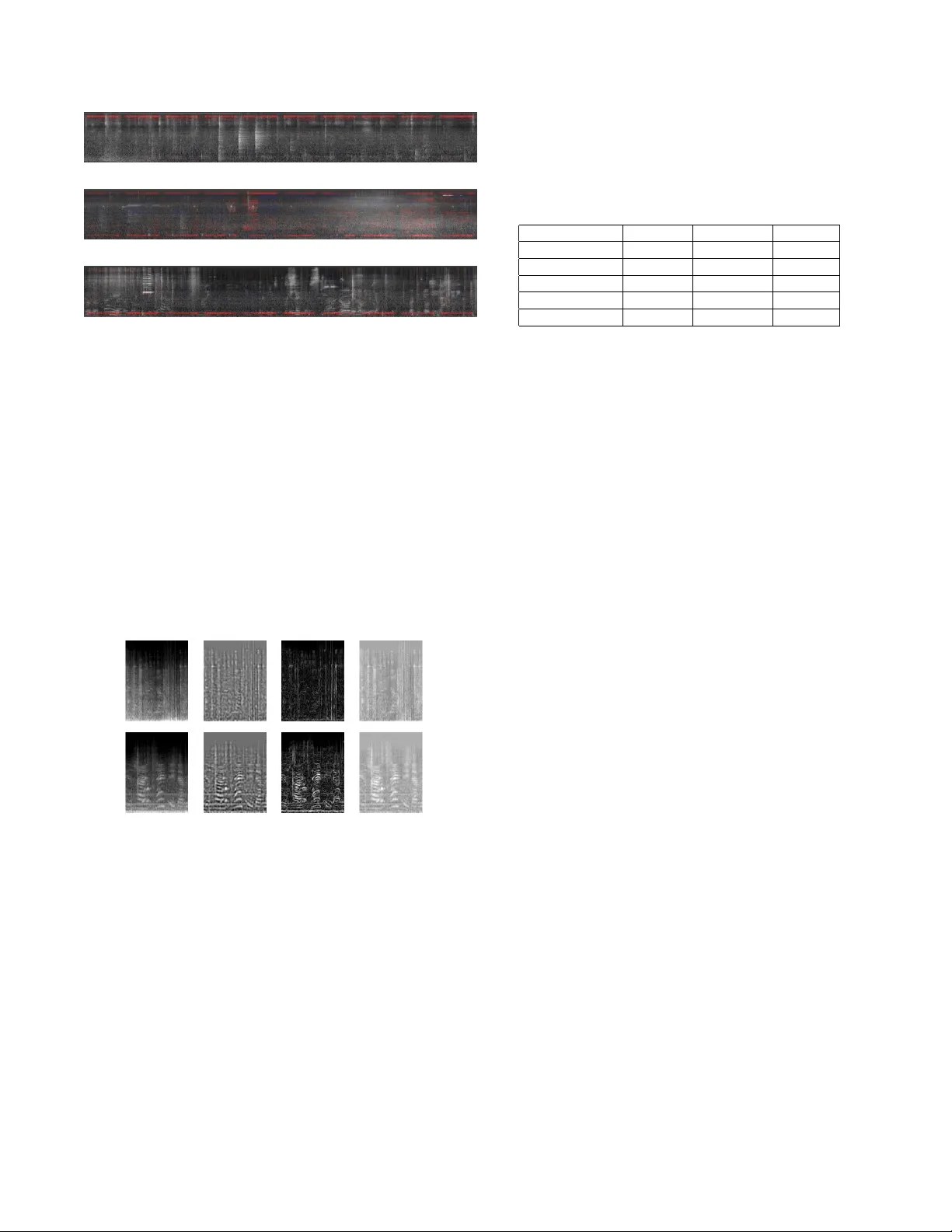
ENHANCING SOUND TEXTURE IN CNN-B ASED A COUSTIC SCENE CLASSIFICA TION Y uzhong W u, T an Lee Department of Electronic Engineering, The Chinese Uni versity of Hong K ong, Hong K ong SAR, China ABSTRA CT Acoustic scene classification is the task of identifying the scene from which the audio signal is recorded. Con volutional neural network (CNN) models are widely adopted with prov en successes in acoustic scene classification. Howe ver , there is little insight on how an au- dio scene is perceiv ed in CNN, as what hav e been demonstrated in image recognition research. In the present study , the Class Activ a- tion Mapping (CAM) is utilized to analyze how the log-magnitude Mel-scale filter-bank (log-Mel) features of dif ferent acoustic scenes are learned in a CNN classifier . It is noted that distinct high-energy time-frequency components of audio signals generally do not cor- respond to strong activ ation on CAM, while the background sound texture are well learned in CNN. In order to make the sound texture more salient, we propose to apply the Dif ference of Gaussian (DoG) and Sobel operator to process the log-Mel features and enhance edge information of the time-frequency image. Experimental results on the DCASE 2017 ASC challenge show that using edge enhanced log-Mel images as input feature of CNN significantly impro ves the performance of audio scene classification. Index T erms — Con volutional neural network, acoustic scene classification, sound texture, class acti vation map, edge enhance- ment 1. INTRODUCTION Large amount of multimedia information becomes easily accessi- ble nowadays. The performance of speech and image recognition systems has been significantly improved with the use of deep neu- ral networks and exploding amount of training data. Audio-related tasks, e.g., Acoustic Scene Classification (ASC) [1, 2, 3], Sound Event Detection (SED) [4, 5, 6] and Audio T agging [7, 8, 9, 10], hav e also received increasing attention in recent years. The y have many real-world applications. For example, context-aw are mobile devices could provide better responses to their users in accordance with the acoustic scene. A smart home-monitoring system could de- tect unusual incidences by using audio. An audio search engine is able to retriev e information efficiently from massi ve online record- ings. Acoustic scene classification (ASC) is the process of identify- ing the type of acoustic en vironment (scene) where a given audio signal was recorded. It has been a major task in the IEEE AASP Challenge on Detection and Classification of Acoustic Scenes and Events (DCASE) since 2013. In the 2017 ASC challenge, most of the best-performing models were based on con volutional neural net- works (CNN). Mun et al. [11] addressed the problem of data in- sufficienc y and proposed to use the Generati ve Adversarial Network (GAN) [12] to augment training data. Han et al. [13] was focused on preprocessing of input features. Fusion of CNN models with prepro- cessed input features led to improv ed overall model performance. Despite the clearly demonstrated effectiv eness of CNN-based models in the ASC task, there is little insight on ho w an audio scene is perceived in a CNN model. Whilst similar issue has been ex- tensiv ely explored in image classification. In [14], Zeiler & Fergus used the De-con volutional Netw ork [15] to visualize and understand CNN. Springenberg et al. applied the guided backpropagation [16] to obtain sharp visualization of descriptiv e image regions. The Class Activ ation Mapping (CAM) [17] w as proposed as a means of high- lighting the discriminativ e image regions for specific output classes in CNNs with global average pooling. Selvaraju et al. dev eloped a generalized version of CAM, named the Gradient-weighted Class Activ ation Mapping (Grad-CAM) [18], which could be applied to a broader range of CNN models. The input of an audio classification model is usually a time- frequency representation extracted from the raw audio waveform. Among the v arious types of time-frequency representations, the logarithmic-magnitude Mel-scale filter bank (abbre viated as log- Mel) feature is widely adopted. Similar to spectrogram, a log-Mel feature is a visual representation of the frequency content of sounds as they vary with time. Given an audio signal with audible sound ev ents such as “bird singing”, “speech”, “applause”, these sound ev ents can also be identified in the corresponding log-Mel feature based on their distinct visual patterns. From this perspective, we may call a log-Mel feature as an image. V isualization of CAM using the log-Mel “image” allows the comparison between machine perception and human interpretation. In this paper, we present an attempt to understand ho w CNN models learn to identify an acoustic scene from log-Mel feature rep- resentations. The in vestigation starts with benchmark systems with log-Mel features and dif ferent CNN models. The method of CAM is used to pro vide visualization of the CNN activ ation beha vior with re- spect to input features. The observed CAMs for acoustic scene data suggest that CNN classification models tend to emphasize on the ov erall background sound texture of log-Mel input features, whilst individual sound events in the scene are of less importance. Hence we propose to use the Dif ference of Gaussian (DoG) and the So- bel operator to pre-process the log-Mel feature to make the back- ground texture information more salient. W e also use the method of background drift removing with medium filter as described in [13] as a comparison to our methods. These texture-enhanced features demonstrate an improv ed performance on ASC. 2. BA CKGR OUND 2.1. Class Activation Mapping The class activ ation mapping [17] highlights the class-specific dis- criminativ e regions in the input image. It can help understand the CNN behavior and visualize the internal representation of CNNs. It can also be used for weakly supervised object localization task. Howe ver , the CAM is only applicable to CNNs with global aver - age pooling (GAP). Suppose we hav e a trained CNN network with global average pooling. There are C output classes. The number of channels in the last con volutional layer is K . The point ( x, y ) in the k th feature map before GAP as f k ( x, y ) . The weight in the output layer is denoted as w c k , indicating the importance of the k th feature map for class c . Then the classification score of class c (before the softmax) is giv en by y c = X k w c k X x,y f k ( x, y ) = X x,y X k w c k f k ( x, y ) . (1) Based on equation 1, the spatial elements of class activ ation map M c for class c is gi ven by M c ( x, y ) = X k w c k f k ( x, y ) . (2) The Gradient-weighted Class Acti vation Mapping (Grad-CAM) [18] is a strict generalization of CAM. It replaces the weight of each activ ation map w c k with the average gradient back-propagated to each feature map, which is giv en by α c k = 1 Z X i,j ∂ y c ∂ f k ( i, j ) , (3) where Z is the number of pixels in the feature map. Notice that f k in Grad-CAM can be from an y conv olutional layers in CNN, not limited to the last con volutional layer . Thus, the Grad-CAM can be applied to a larger variety of CNN models, such as those with fully connected layers (e.g. AlexNet, VGG). In this paper, we propose to use Grad-CAM to analyze the trained CNN models for ASC task. Through empirical analysis of class activ ation maps w .r .t. the ground-truth scene classes, we ar- gue that CNN models are more focusing on the overall background sound texture for classifying acoustic scenes. The distinct sound ev ents (foreground) are usually of less importance in classification. 2.2. Sound T extur e T exture is described as an attribute that characterize spatial arrange- ment of pixel intensities in specific regions of an image. In the area of computer vision, texture analysis is a well studied topic [19, 20, 21, 22]. For audio signal, the notion of “sound texture” has not been seri- ously discussed. An visual analogy of sound texture given by Saint- Arnaud et al. [23] is that sound texture is like a wallpaper which has local structure and randomness, while from a large scale the fine structure characteristics must r emain constant. There were a number of studies on sound texture modeling [24, 25, 26], and commonly mentioned sound textures refer to wind, traf fic, and crowd sounds. In an acoustic scene, there exist various sound sources, which contribute to a mixture of di verse sound ev ents. In audio recordings from acoustic scenes, persistent en vironment sounds with certain sound textures, e.g., crowd, traf fic, form background of the scenes. Whilst certain sparsely occurred sound events, e.g., bird singing, hu- man coughing, are more noticeable and could be re garded as distinct foreground sounds. 2.3. Featur e Prepr ocessing Methods 2.3.1. Differ ence of Gaussian The Difference of Gaussian (DoG) is a well-kno wn method of edge detection in image processing. Briefly speaking, the DoG filtering includes two steps: blurring an image using two Gaussian kernels of different standard deviations, and subtracting one blurred image from another to obtain the edge image. The purpose of Gaussian kernel is to suppress the high (spatial) frequency information (which serves as a lo w-pass filter). The value of standard de viation decides the range of frequency being suppressed. DoG essentially acts like a band-pass filter . It remo ves not only high (spatial) frequency noise, but also homogeneous re gions in the image. 2.3.2. Sobel Operator The Sobel operator [27] is commonly used for edge detection in computer vision. It comprises two 3 × 3 con volution k ernels, which are used to obtain the gradient approximations in the horizontal di- rection ( G x ) and vertical direction ( G y ). For an image A , we ha ve G x =   +1 0 − 1 +2 0 − 2 +1 0 − 1   ∗ A, G y =   +1 +2 +1 0 0 0 − 1 − 2 − 1   ∗ A. (4) The gradient approximations in different directions can be combined as G , as the result of Sobel filtering: G = q G 2 x + G 2 y . (5) 2.3.3. Removing Backgr ound Drift Using Medium F ilter Median filtering is useful in distinguish objects in an image with transitional background. By subtracting the medium-filtered image from the original one, the background drift is remov ed and those sharp changes (edges) are preserved [28]. For the ASC task, me- dian filtering was found to be very effecti ve in feature pre-processing [13], though the determination of kernel size for optimal perfor- mance is not straightforward. 3. A COUSTIC SCENE CLASSIFICA TION SYSTEM 3.1. System Design Experiments on scene visualization and classification are all based on the TUT Acoustic Scenes 2017 database [2]. This database was adopted for the DCASE 2017 ASC challenge. It has two subsets: the development dataset (for model training and cross validation) and the ev aluation dataset (for performance evaluation). All audio samples in the dataset are 10 -second long. The y are cut into 1 -second segments with 0 . 5 second overlapping. Short-Time Fourier T ransform (STFT) is applied to each of the 1 -second seg- ments, with windo w length of 25 ms, windo w shift of 10 ms and FFT length of 2048 . 128 -dimension log-Mel filterbank features are de- riv ed from the FFT spectrum for each frame. Feature components of all frequency bins are normalized to hav e zero mean and unit vari- ance based on training data statistics. The CNN model recei ves the log-Mel feature image of a 1 - second segment as the input, and generates a classification score for the se gment. The classification score for a 10 -second audio sample is obtained by av eraging the segment-le vel scores. 3.2. Model Structure W e examine the performance of two different CNN models. The CNN-FC model as detailed in T able 1 is inspired by the AlexNet [29] and VGG [30] model. After the last conv olutional layer , the feature maps are flattened to obtain the input for the fully connected layer . T able 1 : The CNN-FC model structure. Input 1x100x128 1 3x3 Con volution (pad-1, stride-1)-64-BN-ReLu 2 3x3 Max Pooling (stride-2) 3 3x3 Con volution (pad-1, stride-1)-192-BN-ReLu 4 3x3 Max Pooling (stride-2) 5 3x3 Con volution (pad-1, stride-1)-384-BN-ReLu 6 3x3 Con volution (pad-1, stride-1)-256-BN-ReLu 7 3x3 Con volution (pad-1, stride-1)-256-BN-ReLu 8 3x3 Max Pooling (stride-2) Flattening 9 Dropout (p=0.5) 10 Fully Connected (dim-2048)-BN-ReLU 11 Dropout (p=0.5) 12 Fully Connected (dim-2048)-BN-ReLU 13 15-way SoftMax T able 2 : The CNN-GAP model structure. Input 1x100x128 1 3x3 Con volution (pad-1, stride-1)-64-BN-ReLu 2 3x3 Max Pooling (stride-2) 3 3x3 Con volution (pad-1, stride-1)-192-BN-ReLu 4 3x3 Max Pooling (stride-2) 5 3x3 Con volution (pad-1, stride-1)-384-BN-ReLu 6 3x3 Con volution (pad-1, stride-1)-256-BN-ReLu 7 3x3 Con volution (pad-1, stride-1)-256-BN-ReLu 8 3x3 Max Pooling (stride-2) 9 Global A verage Pooling 10 15-way SoftMax The CNN-GAP model described in T able 2 is constructed by re- placing the fully connected part in CNN-FC model with a global a v- erage pooling layer . Global average pooling (GAP) has been proven to be a good regularizer for CNNs in image classification [31]. GAP is also used in CNNs with audio input feature [32, 33, 34, 35]. The same setup for training and testing is adopted for both models unless stated otherwise. 4. VISU ALIZA TION WITH CLASS A CTIV A TION MAPS For a gi ven audio segment ( 1 -second long in this study), the short- time log-MEL features could be viewed as a gray-scale image, with the x axis and the y axis representing time and frequency respec- tiv ely . The image is combined with class activation maps for lo- calizing the discriminativ e time-frequency regions. The activ ations are deriv ed for the ground-truth scene class, and thus can be used to represent the input patterns learned by the CNN. The proposed CAM visualization of audio segment is created by mixing 3 image components. The first component is the gray- scale log-MEL image. The time-frequency regions that positively influence the classification score of the ground-truth scene class are indicated by a semi-transparent image in red color . The negativ e ac- tiv ations are viewed as another semi-transparent image of blue color . Being different from [18], both positive and negati ve acti vations are included for the observation of acoustic scene features. Figure 1 giv es a few examples of gradient-weighted CAM visu- alization deriv ed from the 7 th layer feature maps in CNN-FC model. These 10 -second audio samples are from the training set of DCASE 2017 dataset. In Figure 1b, the white horizontal lines during the first 3 seconds (inside the green dashed line rectangle) are “bird singing” sounds. It is noted that these distinct sound events are not associ- ated with strong positiv e (red) or negati ve (blue) activ ation. In other words, in CNN classification, these sounds are not regarded as rep- resentativ e patterns for the residential area scene. Figure 2 sho ws the examples of CAM visualization derived from the 7 th layer feature maps in CNN-GAP model. As we can see from these examples, the magnitudes of positi ve activations are much higher than those of negati ve acti v ations. The activ ations are concentrated on a few frequency bins, unlike the CNN-FC model. In addition, the e ye-catching bright lines (fore ground sounds) in the log-MEL images are associated with low activ ation intensity . This suggests that the CNN-GAP model performs classification based on the background “texture” of input image. It frequently happens that the regions of distinct sound ev ents in the log-MEL images have small activ ation intensity , which might be counter -intuitiv e. Howe ver , further inv estigation is needed to find out if these sound ev ents are really trivial for classification, or it is because the CNN models fail to learn these patterns. (a) metro station (b) residential area (c) train Fig. 1 : CAM visualizations w .r .t the ground-truth scene classes. They are derived from the CNN-FC model with log-Mel input. The 3 audio samples are recorded in (a) metro station, (b) residential area and (c) train respecti vely . High energy regions (distinct sound ev ents) are not strongly activ ated. It seems that the model is trying to learn the texture of background sounds. 5. ENHANCING THE EDGE INFORMA TION IN LOG-MEL IMA GES 5.1. Edge-Enhanced Featur es W e propose to use DoG and Sobel operator to enhance the edge in- formation in the input images, making the background texture more salient. Figure 3 gi ves a few e xamples of edge-enhanced images and the corresponding unenhanced ones. T o obtain the DoG enhanced image, we apply Gaussian filter with standard deviation 1 to the original log-Mel image. Then we apply another Gaussian filter with standard deviation √ 2 on the orig- inal image to obtain another blurred image. Subtraction between these two blurred image gi ves the result of DoG. DoG is able to re- mov e high spatial-frequency components and homogeneous regions of images. The result of Sobel operator is an image with pixel values be- ing equal to the gradient magnitudes of the respective pix els in the (a) metro station (b) residential area (c) train Fig. 2 : CAM visualizations w .r .t the ground-truth scene classes. They are deriv ed from the CNN-GAP model with log-Mel input. The audio samples are the same as those in Figure 1. Different from CNN-FC model, there is little negati ve acti vation for CAMs deri ved from CNN-GAP model. original image. Comparing to DoG, the images enhanced by Sobel operator hav e more fine-grained texture. The above mentioned edge-enhanced images are compared to the one obtained by median filtering. The kernel size of medium filter is empirically set to (51 , 7) where 51 refers to time frames (about 0 . 5 second) and 7 refrs to frequency bins. It is noted that median filtering process has a high computation cost, i.e., requiring to calculate the median of each (51 , 7) input windo w for each output pixel. Fig. 3 : Illustration of edge-enhanced input features for CNNs. (From left to right) First column: Original log-Mel image; second column: edge-enhanced images with DoG; third column: edge-enhanced im- ages with Sobel operator; fourth column: background drift removed images with medium filter . 5.2. Evaluating the Edge-Enhanced Features T able 3 shows the accuracy (averaged ov er 3 trials) for differ - ent types of input features. The “LogMel-128” means the 128 dimensional log-Mel feature, which is considered as benchmark feature. “DoG” and “Sobel” refer to the DoG enhanced and Sobel operator enhanced LogMel-128 features, respectively . “Medium” refers to the background-drift-remov ed LogMel-128 feature (using medium filter). The baseline system accuracy is provided by the DCASE 2017 ASC challenge [36]. It can be seen that applying edge-enhancement techniques leads to significant improvement of T able 3 : Experiment results for CNN-FC and CNN-GAP models trained with different input features. The ev aluation data in TUT Acoustic Scenes 2017 database is used for ev aluation. T able ele- ment is the overall classification accuracy (averaged over 3 trials). The accuracy for the baseline setup is from the DCASE 2017 ASC challenge [36]. Feature \ Model CNN-FC CNN-GAP Baseline Baseline - - 0 . 610 LogMel-128 0 . 658 0 . 681 - DoG 0 . 720 0 . 722 - Sobel 0 . 701 0 . 716 - Medium 0 . 757 0 . 754 - classification performance. W e also check the CAM visualizations of CNN models with the edge-enhanced input images, and the ob- servations in Section 4 are still valid. While the CNN-FC model and CNN-GAP model are dif ferent in visualized patterns of CAM, they show similar performance gi ven the same input feature. While the performance of using “DoG” feature is not as good as the “Medium” feature, DoG is computationally much more effi- cient than median filtering. For edge-enhanced features from 100 log-Mel images of size (1000 , 128) , computing “Medium” features takes 272 . 02 seconds with kernel size (51 , 7) in our computer . If the kernel size is changed to (3 , 3) , the computation time is 5 . 7 seconds. On the other hand, applying DoG and Sobel operator takes 0 . 46 and 0 . 30 second respecti vely . 6. CONCLUSION In this paper , we illustrate the use of class activ ation mapping for analysis of CNN beha vior towards audio features. W e find that the distinct sound e vents in log-Mel features are usually not re garded as representativ e patterns of acoustic scenes. Regarding ASC task as a sound texture classification problem, we use the DoG, Sobel opera- tor and background drift removing to enhance the edge information in the log-Mel image. Using these methods, the model performance is improv ed significantly compared to the benchmark. 7. REFERENCES [1] D. Barchiesi, D. Giannoulis, D. Stowell, and M. D. Plumbley , “ Acoustic scene classification: Classifying environments from the sounds they produce, ” IEEE Signal Pr ocessing Magazine , vol. 32, no. 3, pp. 16–34, May 2015. [2] A. Mesaros, T . Heittola, and T . V irtanen, “TUT database for acoustic scene classification and sound ev ent detection, ” in 24th Eur opean Signal Pr ocessing Conference 2016 , Budapest, Hungary , 2016. [3] J. T . Geiger, B. Schuller , and G. Rigoll, “Large-scale audio feature extraction and svm for acoustic scene classification, ” in 2013 IEEE W orkshop on Applications of Signal Processing to Audio and Acoustics , Oct 2013, pp. 1–4. [4] T . Heittola, A. Mesaros, A. Eronen, and T . V irtanen, “Context- dependent sound ev ent detection, ” EURASIP Journal on Au- dio, Speech, and Music Pr ocessing , vol. 2013, no. 1, pp. 1, Jan 2013. [5] E. Cakir, T . Heittola, H. Huttunen, and T . V irtanen, “Poly- phonic sound ev ent detection using multi label deep neural net- works, ” in 2015 International Joint Conference on Neural Net- works (IJCNN) , July 2015, pp. 1–7. [6] G. Parascandolo, H. Huttunen, and T . V irtanen, “Recurrent Neural Networks for Polyphonic Sound Event Detection in Real Life Recordings, ” ArXiv e-prints , Apr . 2016. [7] S. Hershey , S. Chaudhuri, D. P . W . Ellis, J. F . Gemmeke, A. Jansen, et al., “CNN architectures for large-scale audio clas- sification, ” in International Confer ence on Acoustics, Speech and Signal Pr ocessing . 2017. [8] Q. Kong, Y . Xu, W . W ang, and M. D. Plumbley , “ A joint detection-classification model for audio tagging of weakly la- belled data, ” 2017 IEEE International Confer ence on Acous- tics, Speech and Signal Pr ocessing , pp. 641–645, 2017. [9] Y . Xu, Q. Huang, W . W ang, P . Foster , S. Sigtia, et al., “Unsu- pervised feature learning based on deep models for environ- mental audio tagging, ” IEEE/A CM T ransactions on Audio, Speech, and Language Pr ocessing , vol. 25, no. 6, pp. 1230– 1241, June 2017. [10] E. Cakir , T . Heittola, and T . V irtanen, “Domestic audio tagging with con volutional neural networks, ” T ech. Rep., DCASE2016 Challenge, September 2016. [11] S. Mun, S. Park, D. Han, and H. Ko, “Generati ve adversar- ial netw ork based acoustic scene training set augmentation and selection using SVM hyper-plane, ” T ech. Rep., DCASE2017 Challenge, September 2017. [12] I. Goodfello w , J. Pouget-Abadie, M. Mirza, B. Xu, D. W arde- Farle y , et al., “Generativ e adversarial nets, ” in Advances in Neural Information Processing Systems 27 , pp. 2672–2680. Curran Associates, Inc., 2014. [13] Y . Han and J. Park, “Conv olutional neural networks with bin- aural representations and background subtraction for acous- tic scene classification, ” in Pr oceedings of the Detection and Classification of Acoustic Scenes and Events 2017 W orkshop , Nov ember 2017, pp. 46–50. [14] M. D. Zeiler and R. Fergus, “V isualizing and Understanding Con volutional Netw orks, ” ArXiv e-prints , Nov . 2013. [15] M. D. Zeiler , G. W . T aylor , and R. Fergus, “ Adaptiv e decon vo- lutional networks for mid and high level feature learning, ” in 2011 International Confer ence on Computer V ision , Nov 2011, pp. 2018–2025. [16] J. T . Springenberg, A. Dosovitskiy , T . Brox, and M. Riedmiller , “Striving for Simplicity: The All Con volutional Net, ” ArXiv e- prints , Dec. 2014. [17] B. Zhou, A. Khosla, A. Lapedriza, A. Oliv a, and A. T or- ralba, “Learning Deep Features for Discriminative Localiza- tion, ” ArXiv e-prints , Dec. 2015. [18] R. R. Selvaraju, M. Cogswell, A. Das, R. V edantam, D. P arikh, et al., “Grad-CAM: V isual Explanations from Deep Networks via Gradient-based Localization, ” ArXiv e-prints , Oct. 2016. [19] L. Liu and P . Fieguth, “T exture classification from random features, ” IEEE T ransactions on P attern Analysis and Machine Intelligence , v ol. 34, no. 3, pp. 574–586, March 2012. [20] D. Puig, M. A. Garcia, and J. Melendez, “ Application- independent feature selection for texture classification, ” P at- tern Recogn. , v ol. 43, no. 10, pp. 3282–3297, Oct. 2010. [21] X. Chen, X. Zeng, and D. van Alphen, “Multi-class feature selection for texture classification, ” P attern Recogn. Lett. , vol. 27, no. 14, pp. 1685–1691, Oct. 2006. [22] A. H. Bhalerao and N. M. Rajpoot, “Discriminant feature se- lection for texture classification, ” in Pr oc. British Mac hine V i- sion Confer ence , 2003. [23] N. Saint-arnaud and K. Popat, “ Analysis and synthesis of sound te xtures, ” in Readings in Computational Auditory Scene Analysis , 1995, pp. 125–131. [24] D. Schwarz, “State of the art in sound texture synthesis, ” in Pr oceedings of the 14th International Conference on Digital Audio Ef fects , September 2011. [25] M. Athineos and D. P . W . Ellis, “Sound texture modelling with linear prediction in both time and frequency domains, ” in 2003 IEEE International Confer ence on Acoustics, Speech, and Sig- nal Pr ocessing , 2003. [26] W . Liu, G. Liu, X. Ji, J. Zhai, and Y . Dai, “Sound texture gener- ativ e model guided by a lossless mel-frequency con volutional neural netw ork, ” IEEE Access , v ol. 6, pp. 48030–48041, 2018. [27] I. Sobel and G. Feldman, “ An isotropic 3x3 gradient operator , ” in Stanfor d Artificial Intelligence Pr oject (SAIL) , 1968. [28] A. W . Moore and J. W . Jorgenson, “Median filtering for re- mov al of lo w-frequency background drift, ” Analytical Chem- istry , vol. 65, no. 2, pp. 188–191, 1993. [29] A. Krizhevsk y, “One weird trick for parallelizing conv olu- tional neural networks, ” ArXiv e-prints , Apr . 2014. [30] K. Simonyan and A. Zisserman, “V ery Deep Conv olutional Networks for Lar ge-Scale Image Recognition, ” ArXiv e-prints , Sept. 2014. [31] M. Lin, Q. Chen, and S. Y an, “Network In Netw ork, ” ArXiv e-prints , Dec. 2013. [32] Y . Sakashita and M. Aono, “ Acoustic scene classification by ensemble of spectrograms based on adaptiv e temporal di vi- sions, ” T ech. Rep., DCASE2018 Challenge, September 2018. [33] M. Dorfer , B. Lehner, H. Eghbal-zadeh, H. Christop, P . Fabian, et al., “ Acoustic scene classification with fully con volutional neural networks and I-vectors, ” T ech. Rep., DCASE2018 Chal- lenge, September 2018. [34] H. Zeinali, L. Burget, and H. Cernocky , “Con volutional neu- ral networks and x-vector embedding for dcase2018 acoustic scene classification challenge, ” T ech. Rep., DCASE2018 Chal- lenge, September 2018. [35] Y . W u and T . Lee, “Reducing model complexity for DNN based large-scale audio classification, ” in 2018 IEEE Interna- tional Confer ence on Acoustics, Speech and Signal Pr ocessing , Calgary , Canada, 2018. [36] T . Heittola and A. Mesaros, “DCASE 2017 challenge setup: T asks, datasets and baseline system, ” T ech. Rep., DCASE2017 Challenge, September 2017.