Joint Beam and Channel Tracking for Two-Dimensional Phased Antenna Arrays

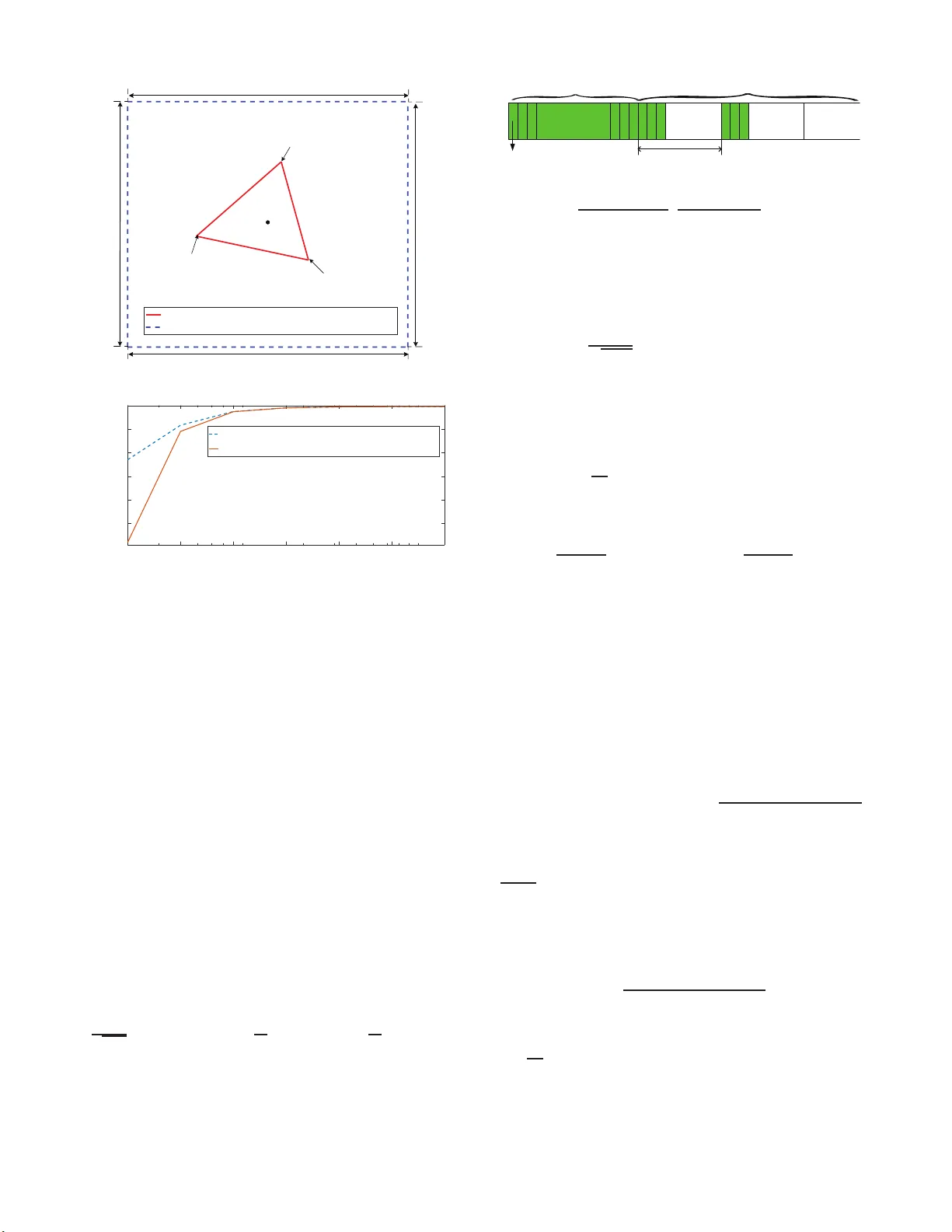
Joint Beam and Chann el T racking for T wo-Di mensional Phased Antenna Arrays Y u Liu ∗ , Jiahui Li ∗ , Y in Sun § , Shidong Zhou ∗ ∗ Dept. of EE, Tsinghua Univ ersity , Beijing, 100084 , China § Dept. of E CE, Auburn University , Auburn AL, 368 49, U.S.A Abstract —Analog beamforming is a low-cost architecture f or millimeter -wa v e (mmW av e) mobile communications. Howe ve r , it has two disadvantages f or ser ving fast mobility u sers: (i) the mmW av e beam in t he wireless channel and the beam steered by analog beamf orming hav e small angular spreads which are difficult to align with each oth er and (ii) the receiv er can only observ e the mmW av e ch annel in one beam direction and rely on beam-probing algorithms to check other directions. In this paper , we develo p a beam probing and tracking algorithm th at can ef- ficiently track fast-moving mmW a v e beams in three-dimensional (3D) space. This algorithm has se vera l salient features: (1) fading channel supportive: it can simul taneously track the ch an n el coefficient and two-dimensional (2D) beam direction in fading channel en vir onments; (2) low probing overhead: it achie ves the minimum p robing requirement for joint b eam and channel tracking; (3) fast tracking sp eed and high tracking accurac y: its tracking error con verges to the minimum Cram ´ er -Rao lower bound (CRLB) in static scenarios in theory and it outperform s sev eral existing trackin g algorithms with lower tracking error and faster tracking speed in simulations. I . I N T R O D U C T I O N Due to the lo w ha rdware cost and en ergy co n sumption, analog bea m forming is often used in m mW a ve mo bile com- munication s to provide large array g ains [1], [2]. Howev er , the beam steered by analog beamfo r ming has small angular spreads. Slight misalignme n t can cause sev ere energy loss. Accurate alignment can be achieved by b eam train ing at the expense of large pilot overhead in static or quasi-static sce- narios. Nev ertheless, this p rice is unacceptable in fast-moving en vironmen ts. Therefore , efficient beam track in g is important for serving fast mobility u sers in mmW av e communication. Some beam tracking metho d s has been proposed [3]–[5], utilizing historical observations and e stima tio ns to ob tain current estimate. Desp ite this, the analo g b eamform ing vectors are not optimized in those tracking algorithm s, resulting in a waste of transmission energy . A be am tracking algorithm is propo sed in [6], trying to optimize the ana lo g beamformin g vectors, assuming th e chan n el coefficient is kn own. In [7], the autho rs start to jointly track the channel coefficient and beam direction with optimal a n alog beamformin g vectors. T he theorems of convergence and optimality are established for joint tracking. Howe ver , all these algorithms ar e b ased on unifor m linear array (ULA) antenn as, which can o n ly support one-dim ensional (1D) beam tr acking. While in se veral m obile scenarios, e.g., u nmanne d a e rial vehicle (UA V) scen arios [8], the beam may also come from d ifferent horizo n tal an d vertical directions. Hence, we need to dynamic a lly track the two- dimensiona l (2 D) beam direction with 2D p hased antenna arrays. This p roblem is ch allenging du e to the following three reasons: (i) with analo g beamfo rming, we ca n only obtain part of the system information through one observation. (ii) W e n eed to jo intly trac k cha nnel co efficient and 2D be a m direction and the analog bea m formin g vectors also need to be adjusted. The r efore, it is a d y namic joint optimization p rob- lem with sequ ential analog beamfo rming vectors and th e se analog bea m forming vectors also need to be optimized. (iii) Compared with 1D beam direction, more analog beam f orming vectors are required when tr acking 2D be a m direction. As a result, the op timization dimen sion greatly increases. In this paper, we design a join t beam and chann el tracking algorithm for 2D phased antenna arrays to handle the prob le m above. The m a in co ntributions and r esults are summar ized as follows: • This alg orithm can achiev e th e minimu m probin g over- head for join t bea m an d ch annel tra c k ing. • In static scenar ios, we get the p erforman ce bound, i.e., the minimum CRLB by optimizing th e ana lo g b eamform ing vectors under s ome constrain ts. A general way to ge nerate the optimal analog beamf orming vector s is prop osed with a seq u ence of parameters. Th ese param eters ar e p roved to be asymptotically optimal in dif ferent conditions, e. g., channel coefficients, an d path d irections, as the n umber of antennas gr ows to infin ity . • W e prove th a t ou r a lgorithm can conver ge to the mini- mum CRLB with high probability in static scenarios. • Simulation results show that our algorith m appro aches the minimum CRLB quickly in static scenarios. In dyn amic scenarios, our algor ithm can achieve lower tra c king error and faster tracking sp e ed comp ared with sev eral existing algorithm s. I I . S Y S T E M M O D E L W e consider a mmW ave receiver equipp ed with a planar phased antenna array 1 , as shown in Fig. 1. T he planar array consists of M × N antenna elemen ts that are p laced in a rectangu la r area, with a distance d 1 ( d 2 ) between neighbor ing 1 Note that tracking is needed at both the transmitte r an d recei v er . Ho we ve r , consideri ng the transmitter -recei ver recipro city , the beam and channel tracki ng of bot h sides have similar designs. Hence, we focus on beam and channel tracki ng on the rece i ve r side. x y z q k f k m M n N 1 d 2 d Fig. 1. 2D phased antenna array . antenna elemen ts alon g x -axis ( y -axis) 2 . Th e an tenna elements are con nected to th e sam e RF ch ain throug h different ph a se shifters. Th e system is time-slotted. T o estimate and track the directio n of the inc oming beam, the tran smitter sends q pre- determined pilot symbo ls s p in eac h time slot, where | s p | 2 = E p is th e tran smit po wer of each pilot symb ol. In mmW a ve channels, only a fe w paths exist due to the weak scattering effect [1]. Becau se the angle spr ead is small and the mm W a ve sy stem is usua lly co nfigured with a large number of anten n as, the inte r action b etween m ulti-paths is relativ ely weak . In other word s, the incomin g bea m paths are usually sparse in space, m aking it p ossible to track ea ch path indep endently [11]. Hence, we focus on the method for tracking one path. Different p aths can b e tracked separately by using the same method. In time-slot k , the direction of the inc o ming bea m path is denoted by ( θ k , ϕ k ), where θ k ∈ [0 , π/ 2] is the elevation ang le of arriv al (Ao A) and ϕ k ∈ [ − π , π ) is the azim uth AoA. The chann e l vector of this path is h k = β k a ( x k ) , (1) where β k = β re k + j β im k is th e complex chan nel coefficient, x k = [ x k, 1 , x k, 2 ] T = h M d 1 cos( θ k ) cos( ϕ k ) λ , N d 2 cos( θ k ) sin( ϕ k ) λ i T is th e direction par ameter vector determined b y ( θ k , ϕ k ), a ( x k ) = [ a 11 ( x k ) · · · a 1 N ( x k ) a 21 ( x k ) · · · a M N ( x k )] T (2) is the steering vector with a mn ( x k ) = e j 2 π ( m − 1 M x k, 1 + n − 1 N x k, 2 ) ( m = 1 , · · · , M ; n = 1 , · · · , N ) , and λ is the wav elength. Let w k,i be the analog beamf o rming vector for receiving the i -th ( i = 1 , · · · , q ) pilot sym bol in time-slot k , given by w k,i = 1 √ M N a ( x k + ∆ k,i ) , (3) where e ∆ k,i is the directio n parameter offset cor respond in g to w k,i . After phase shif ting and com bining, the o bservation at the baseband o utput o f RF chain is g i ven by y k,i = w H k,i h ( x k ) s p + z k,i = s p β k w H k,i a ( x k ) + z k,i , (4) ψ k ,  β re k , β im k , x k, 1 , x k, 2  T where z k,i ∼ C N (0 , σ 2 ) is an i.i.d. circula r ly symmetric comp lex Ga u ssian random variable. Define ψ k ,  β re k , β im k , x k, 1 , x k, 2  T as the chan nel p arameter 2 T o obta in differen t resolutions in horizontal direc tion and vertic al direct ion, the antenna numbers along diffe rent directions may not be the same, i.e., M 6 = N [9]. T o suppress sidelobe, th e antennas may be unequally spaced, i.e., d 1 6 = d 2 [10]. vector in time-slot k , W k , [ w k, 1 , . . . , w k,q ] as the analog beamfor ming matrix, an d z k , [ z k, 1 , . . . , z k,q ] as the noise vector . Then the cond itional pro bability density function of the o bservation vector y k , [ y k, 1 , . . . , y k,q ] T is g iv en by p ( y k | ψ k , W k ) = 1 π q σ 2 q e − k y k − s p β l W H k a ( x ) k 2 2 σ 2 . (5) In time-slot k , the receiver n e e ds to choo se an analog beam- forming matrix W k and obtain an estimate ˆ ψ k ,  ˆ β re k , ˆ β im k , ˆ x k, 1 , ˆ x k, 2  T of the chann el par ameter vector Ψ k . From a control system perspective, ψ k is the system state, ˆ ψ k is the estimate of the system state, th e ana lo g beamf orming matrix W k is the co ntrol action and y k is a no n-linear noisy observation determined by the system state and contro l action . I I I . P RO B L E M F O R M U L AT I O N A N D O P T I M A L B E A M F O R M I N G M AT R I X A. Pr oblem F ormulation Let ζ = ( W 1 , W 2 , . . . , ˆ ψ 1 , ˆ ψ 2 , . . . ) denote a beam and channel track ing scheme. W e consid e r a particular set Ξ of causal beam tracking policies: in time-slot k , the ana log beamfor ming matrix W k and estimate ˆ ψ k are based on the previously used ana lo g beamformin g matrix W 1 , · · · , W k − 1 and historica l o bservations y 1 , · · · , y k − 1 . Hence , in k -th time- slot, the beam and channe l tracking problem is fo rmulated as: min ζ ∈ Ξ 1 M N E     ˆ h k − h k    2 2  (6) s.t. E h ˆ h k i = h k , (7) (1) − (4) , where the constrain t (7) en sures that ˆ h k , ˆ β k a ( ˆ x k ) is an unbiased estimation of the chann el vector h k = β k a ( x k ) and the constraints (1)-(4) ensure the steering vector form of analog beamforming vector s. Problem (6) is difficult to solve o ptimally d u e to se veral r ea- sons: (i) it is a con strained partially observed Markov decision process (C-POMDP) that is usu ally quite difficult to so lve. (ii) The ana log beam forming matrix W k and the estimate ˆ ψ k need to be op timized. However , both the o ptimization of W k and ˆ ψ k are n on-co nvex problems. Before g i ving so me theoretical results of problem (6), we will first study the p ilot overhead n eeded for b eam and channel tracking in 2D phased antenna arr ays. B. How Many Pilo ts A r e Needed? According to [ 7], two pilots in each time-slot are sufficient to join tly track the chan nel coefficient and 1D beam direction . When tr a cking the horizontal and v ertical beam direction simultaneou sly , four pilots are feasible by separately using two pilots to tr ack e ach dimen sion of the 2 D beam direction . Howe ver , with fou r pilots, the chann el coefficient is updated twice in each time-slot, po ssibly leading to redu ndancy . Hence, we can jointly track chan nel coefficient and 2D beam direction to f urther r educe pilot overhead. When track ing the channel paramete r s join tly , fou r r eal vari- ables (i.e., th e real p art β re k and imaginary part β im k of channel coefficient β k and the two direction parameters x k, 1 , x k, 2 ) need to be estimated. Th en the following lemma is prop o sed to help d e termine the smallest q : Lemma 1. If the analog beamforming vecto rs ar e steering vectors, i.e., w k,i = 1 √ M N a ( x + ∆ k,i ) , then a t least q observa- tions ar e needed to estimate q + 1 r eal variables in time-slot k . Pr o of. See Appendix A. Lemma 1 tells us at least thr e e observations are required in each time-slot to estimate fo ur real variables. Hen c e, the smallest p ilot nu m ber in each time-slot is q = 3 , i.e. , the analog beamforming ma tr ix W k = [ w k, 1 , w k, 2 , w k, 3 ] . C. Lower Bound o f T r ac king Err or The huge c h allenge to solve prob lem (6) optimally makes it hard to comp lete in just o ne paper . T herefor e, we perfor m some theo retical analysis f or static scen arios as the first step in this p a per . Consider the problem of trac k ing a static bea m, where ψ k = ψ ,  β re , β im , x 1 , x 2  T for all time-slots. The Cram ´ er- Rao lo wer bou nd theo ry gives th e lo wer boun d of the u nbiased estimation error accor ding to [12]. Based on this, we intr oduce the f ollowing lemma to obtain the lower bou nd of trac k ing error: Lemma 2. The MSE of channel vector in (6) is lower b ound e d as follows: 1 M N E     ˆ h k − h k    2 2  (8) ≥ 1 M N T r    k X l =1 I ( ψ , W l ) ! − 1 M X m =1 N X n =1  v H m,n v m,n     , wher e v m,n ,  1 , j, j 2 π m − 1 M β , j 2 π n − 1 N β  and th e F isher information matrix I ( ψ , W k ) is given by I ( ψ , W k ) , − E  ∂ l og p ( y k | ψ , W k ) ∂ ψ · ∂ l og p ( y k | ψ , W k ) ∂ ψ T  (9) = 2 | s p | 2 σ 2     k g k k 2 2 0 Re { g H k ˜ g k 1 } Re { g H k ˜ g k 2 } 0 k g k k 2 2 Im { g H k ˜ g k 1 } Im { g H k ˜ g k 2 } Re { g H k ˜ g k 1 } Im { g H k ˜ g k 1 } k ˜ g k 1 k 2 2 Re { ˜ g H k 1 ˜ g k 2 } Re { g H k ˜ g k 2 } Im { g H k ˜ g k 2 } Re { ˜ g H k 1 ˜ g k 2 } k ˜ g k 2 k 2 2     , with g k = W H k a ( x ) , ˜ g k 1 = β W H k ∂ a ( x ) ∂ x 1 , and ˜ g k 2 = β W H k ∂ a ( x ) ∂ x 2 . Pr o of. See Appendix B. The CRLB in (8) is a function of the analog beamformin g matrices W 1 , . . . , W k . I t is hard to optimize so many beam- forming matrices simultaneo u sly . Suppo se that W 1 = W 2 = . . . = W k . Then we can get the minimu m CRLB under this constriant, gi ven by I min ( ψ ) = min W 1 ,..., W k 1 M N T r    k X l =1 I ( ψ , W l ) ! − 1 M X m =1 N X n =1  v H m,n v m,n     = min W 1 M N T r ( ( k I ( ψ , W )) − 1 M X m =1 N X n =1  v H m,n v m,n  ) . (10) T ABLE I A S Y M P T O T I C A L LY O P T I M A L O FF S E T S . e ∆ ∗ 1 e ∆ ∗ 2 e ∆ ∗ 3 [0 . 0963 , 0 . 5098] T [ − 0 . 5098 , − 0 . 0963] T [0 . 2906 , − 0 . 2906] T Solving pro blem (10) yield s the optimal analog beamforming matrix W ∗ = [ w ∗ 1 , w ∗ 2 , w ∗ 3 ] : w ∗ i = 1 √ M N a ( x + ∆ ∗ i ) , i = 1 , 2 , 3 , (11) where ∆ ∗ 1 , ∆ ∗ 2 , ∆ ∗ 3 denote the optimal direction param eter offsets. Hence, let W ∗ 1 = W ∗ 2 = · · · W ∗ k = W ∗ and we can obtain th e minimum CRLB by (10). D. Asymptotically Optimal An alog Beamfo rming Matrix Let us consider the op tim al analog beamfor ming matrix W ∗ . In (1 0), three 2D dire c tio n parameter offsets need to be optimized. It is hard to get analytica l re su lts for su c h a six- dimensiona l no n-conve x p roblem. Numerical search is a feasi- ble way to handle the problem. Howe ver , these optimal offsets may be r elated to some system parameters, e.g., channel coefficient β , direction p arameter vector x and anten n a array size M , N . On ce the se system parameters chan ge, nu merical search h as to be re-co n ducted, leadin g to high c omplexity . T o overcome this challen ge, we explor e the proper ties of ∆ ∗ 1 , ∆ ∗ 2 , ∆ ∗ 3 and obtain the following lemma: Lemma 3. The optimal dir e ction parameter offsets ∆ ∗ 1 , ∆ ∗ 2 , ∆ ∗ 3 have the following thr ee p r o perties : 1) ∆ ∗ 1 , ∆ ∗ 2 , ∆ ∗ 3 ar e invariant to the cha n nel coefficient β ; 2) ∆ ∗ 1 , ∆ ∗ 2 , ∆ ∗ 3 ar e in variant to the direction pa rameter vector x ; 3) ∆ ∗ 1 , ∆ ∗ 2 , ∆ ∗ 3 conver ge to con stant values as M , N → + ∞ : e ∆ ∗ i , lim M ,N → + ∞ ∆ ∗ i , i = 1 , 2 , 3 . Pr o of. See Appen dix C. Lemma 3 re veals that ∆ ∗ 1 , ∆ ∗ 2 , ∆ ∗ 3 are on ly related to array size M , N . Hence, th e nume r ical sear c h comp lexity can b e reduced to o ne for a par ticular array size M , N . Even if ∆ ∗ 1 , ∆ ∗ 2 , ∆ ∗ 3 may chan ge for dif ferent a r ray sizes, we can adopt e ∆ ∗ 1 , e ∆ ∗ 2 , e ∆ ∗ 3 to take the place of ∆ ∗ 1 , ∆ ∗ 2 , ∆ ∗ 3 as long as M an d N are sufficiently large. T herefor e , the nu merical search times are reduced to on e. By numer ic a l search in th e main lob e of the directio n parameter vector: B ( x ) , ( x 1 − 1 , x 1 + 1) × ( x 2 − 1 , x 2 + 1) , (12) we can obtain the asym p totically op timal directio n parameter offsets e ∆ ∗ 1 , e ∆ ∗ 2 , e ∆ ∗ 3 in T ABLE I and Fig. 2. W ith these offsets, a general way to generate the asymptotically optimal analog b eamform ing matrix e W ∗ k = [ ˜ w ∗ k, 1 , ˜ w ∗ k, 2 , ˜ w ∗ k, 3 ] is o b- tained to achieve the minimum CRLB as below: ˜ w ∗ k,i = 1 √ M N a  x + e ∆ ∗ i  , i = 1 , 2 , 3 . (13) Asy mpto tically opt imal direc tion param eter offset s Main lobe boundary x * 1 + x Δ % * 2 + x Δ % * 3 + x Δ % 2 2 2 2 Fig. 2. Asymptotica lly opti mal offset s. 2 4 8 16 32 64 128 antenna n um ber M = N 2 2.05 2.1 2.15 2.2 2.25 M N × C RLB CRLB corresponding to offsets in Tab.1 minimum CRLB Fig. 3. Performance of off sets in T ABLE I By ad o pting e ∆ ∗ 1 , e ∆ ∗ 2 , e ∆ ∗ 3 to smaller size an tenna arr ays, we compare the minimu m CRLB and the CRLB corr e sp ond- ing to e ∆ ∗ 1 , e ∆ ∗ 2 , e ∆ ∗ 3 in T ABLE I. As illustrated in Fig. 3, when anten na num ber M = N ≥ 8 , we can approac h the m inimum CRLB with a relative error less than 0 . 1% by using e ∆ ∗ 1 , e ∆ ∗ 2 , e ∆ ∗ 3 . Therefo re, with e ∆ ∗ 1 , e ∆ ∗ 2 , e ∆ ∗ 3 , the minimum CRLB is obtained fo r different b eam dir ections, different channel coefficients and different antenna nu mbers when M = N ≥ 8 . I V . A S Y M P T OT I C A L LY O P T I M A L J O I N T B E A M A N D C H A N N E L T R AC K I N G A. Joint Beam and Channel T racking The prop o sed track in g algorithm is similar to that in [7]. The m ain difference is that we nee d M × N pilots to estimate th e initial dire c tio n parameter offsets and three analog beamfor ming vecto rs to track the time-varying beam direction. Joint Beam and Cha nnel T racking : 1) Coarse Beam Sweeping: As shown in Fig. 4, M × N pilots ar e rece i ved successiv ely . T he analog be a mformin g vector co rrespon ding to the observation ˇ y m,n is ˇ w m,n = 1 √ M N a   (2 m − 1 − M ) d 1 λ , (2 n − 1 − N ) d 2 λ  T  , m = 1 , · · · , M , n = 1 , · · · , N . Th e initial estimate ˆ ψ 0 =  ˆ β re 0 , ˆ β im 0 , ˆ x 0 , 1 , ˆ x 0 , 2  T is o btained by: ˆ x 0 = argmax ˆ x ∈ χ | a ( ˆ x ) H ˇ W ˇ y | , ˆ β 0 = h ˇ W H a ( ˆ x 0 ) i + ˇ y , (14) Ă D a t a Ă P i l o t M N p i l ot s f o r b e a m s w e e p i ng 3 p i l o t s p e r t i m e s l ot f or t r a c k i n g s l o t Ă D a t a Ă Ă Data Data MN pilots for beam sweeping 3 pilots per time-slot for tracking Ă Pilots time-slot Fig. 4. Frame structure. where χ = ( h (2 m − 1 − M 0 ) M d 1 λM 0 , (2 n − 1 − N 0 ) N d 2 λN 0 i T     m = 1 , . . . , M 0 n = 1 , . . . , N 0 ) , M 0 × N 0 is the codeb ook size with M 0 ≥ M and N 0 ≥ N , ˇ y = [ ˇ y 11 , ˇ y 12 · · · , ˇ y M N ] T , ˇ W = [ ˇ w 11 , ˇ w 12 , · · · , ˇ w M N ] , and X + =  X H X  − 1 X H . 2) Beam and channel tracking: I n time-slot k , thr ee pilots ar e received by using analo g beamform ing vectors given below: w k,i = 1 √ M N a  ˆ x k − 1 + e ∆ ∗ i  , i = 1 , 2 , 3 , (15) where ˆ x k , [ ˆ x k, 1 , ˆ x k, 2 ] T and e ∆ ∗ i ( i = 1 , 2 , 3 ) are given by T ABLE I. The estimate ˆ ψ k = h ˆ β re k , ˆ β im k , ˆ x k, 1 , ˆ x k, 2 i is updated by ˆ ψ k = ˆ ψ k − 1 + 2 σ 2 b k I  ˆ ψ k − 1 , W k  -1       Re  s H p e H k ( y k − ˆ y k )  Im  s H p e H k ( y k − ˆ y k )  Re  s H p ˜ e H k 1 ( y k − ˆ y k )  Re  s H p ˜ e H k 2 ( y k − ˆ y k )        , (16) where e k = W H k a ( ˆ x k − 1 ) , ˆ y k = s p ˆ β k − 1 W H k a ( ˆ x k − 1 ) , ˜ e k 1 = ˆ β k − 1 W H k ∂ a ( ˆ x k − 1 ) ∂ x 1 and ˜ e k 2 = ˆ β k − 1 W H k ∂ a ( ˆ x k − 1 ) ∂ x 2 . Here, b k is the step size and will b e specified later . B. Asymptotic Optimality An alysis In the tracking procedur e ( 16), there exist multip le stable points and these stable p oints corr espond to the local optimal points for ou r pro posed a lg orithm. T o stud y these stable poin ts, we re write (1 6) as (17): ˆ ψ k = ˆ ψ k − 1 + b k  f  ˆ ψ k − 1 , ψ k  + ˆ z k  , (17) where f  ˆ ψ k − 1 , ψ k  is d efined as fo llows: f  ˆ ψ k − 1 , ψ k  , E   I  ˆ ψ k − 1 , W k  -1 ∂ l og p  y k | ˆ ψ k − 1 , W k  ∂ ˆ ψ k − 1   = 2 | s p | 2 σ 2 I  ˆ ψ k − 1 , W k  -1         Re n e H k  β k W H k a ( x k ) − ˆ β k − 1 e k  o Im n e H k  β k W H k a ( x k ) − ˆ β k − 1 e k  o Re n ˜ e H k 1  β k W H k a ( x k ) − ˆ β k − 1 e k  o Re n ˜ e H k 2  β k W H k a ( x k ) − ˆ β k − 1 e k  o         , (18) and ˆ z k is g iv en by ˆ z k , I  ˆ ψ k − 1 , W k  -1 ∂ l og p  y k | ˆ ψ k − 1 , W k  ∂ ˆ ψ k − 1 − f  ˆ ψ k − 1 , ψ k  = 2 σ 2 I  ˆ ψ k − 1 , W k  -1       Re  s H p e H k z k  Im  s H p e H k z k  Re  s H p ˜ e H k 1 z k  Re  s H p ˜ e H k 2 z k        . (19) A stable point ˆ ψ k − 1 of f  ˆ ψ k − 1 , ψ k  satisfies two con- ditions: 1 ) f  ˆ ψ k − 1 , ψ k  = 0 ; 2) ∂ f ( ˆ ψ k − 1 , ψ k ) ∂ ˆ ψ T k − 1 is negative definite. Hence, we define the stable points set in tim e-slot k as : S k ,  ˆ ψ k − 1 : f  ˆ ψ k − 1 , ψ k  = 0 , ∂ f ( ˆ ψ k − 1 , ψ k ) ∂ ˆ ψ T k − 1 ≺ 0  . The channe l parameter ψ k is a stable po int: when ˆ ψ k − 1 = ψ k , 1) β k W H k a ( x k ) = ˆ β k − 1 e k in ( 18). Hence, f ( ψ k , ψ k ) = 0 ; 2) ∂ f ( ψ k , ψ k ) ∂ ˆ ψ T k − 1 = − J 4 by derivation, where J 4 is a 4 × 4 identity matrix. Thu s, ∂ f ( ψ k , ψ k ) ∂ ˆ ψ T k − 1 is n egati ve definite. Therefo re, ψ k is a stable point. Other stable points in S k correspo n d to the local optimal points o f the beam and c h annel track ing prob lem, which are without the main lobe B ( x ) . Except f or the channel par ameter vector ψ k , the antenna array gain of other stable points in S k is q u ite low , re sulting in low tracking accu racy . Therefo re, one key c hallenge is to ensure th at the track ing alg orithm conv erges to ψ k rather than o th er stab le po ints. In static scenarios, where S k = S ,  ˆ ψ k − 1 : f  ˆ ψ k − 1 , ψ  = 0 , ∂ f ( ˆ ψ k − 1 , ψ ) ∂ ˆ ψ T k − 1 ≺ 0  , th e c o rrespon ding theo- rems are developed to study the convergence of ou r algorithm. W e adopt the diminishing step-size in (20), given by [14]–[16] b k = ǫ k + K 0 , k = 1 , 2 , · · · (20) where K 0 ≥ 0 and ǫ > 0 . Theorem 1 ( Co n ver gence to a U nique Stable Point ) . I f b k is give n by (20) with ǫ > 0 a nd K 0 ≥ 0 , then ˆ ψ k conver ges to a un iq ue stable point with p r o bability o n e. Pr o of. See Appendix D. Therefo re, for the gen eral step-size in (20), ˆ ψ k conv erges to a u nique stable point. Theorem 2 ( Con ver gence to Dir ection para meter vector x ) . If ( i) the initial estimate o f x is within the main lobe , i.e., ˆ x 0 ∈ B ( x ) , and (ii) b k is given b y (20) with ǫ > 0 , then th er e exis t some K 0 ≥ 0 and C > 0 such that P ( ˆ x k → x | ˆ x 0 ∈ B ( x )) ≥ 1 − 8 e − C | s p | 2 ǫ 2 σ 2 . (21) Pr o of. See Appendix E. At the coarse be a m sweeping stage of o ur prop osed algo- rithm, the initial estimation ˆ x 0 within main lobe B ( x ) in (1 2) can be obtained with h igh probab ility . Under the con d ition ˆ x 0 ∈ B ( x ) , Theorem 2 tells us the p robab ility of ˆ x k → x is related to | s p | 2 ǫ 2 σ 2 . Hence, we can reduce the step-size and increase the transmit SNR | s p | 2 σ 2 to m ake sure th at ˆ x k → x with probability on e. Theorem 3 ( Conv ergence to x with minimum CRLB ) . If (i) ˆ ψ k → ψ an d (ii) b k is given by ( 2 0) with ǫ = 1 an d any K 0 ≥ 0 , then ˆ h k − h k is asymptotically Ga u ssian a nd lim k →∞ k M N E     ˆ h k − h    2 2   ˆ ψ k → ψ  = I min ( ψ ) . (22) 10 1 10 2 10 3 Time-slot number k 10 -4 10 -2 10 0 1 M N E h || ˆ h k − h k || 2 2 i IEEE 802.11ad Extended Kalman Filter Compressed sensing Joint tracking (4 pilots/iteration) Joint tracking (3 pilots/iteration) Minimum CRLB Fig. 5. 1 M N MSE h k in static tracki ng scen arios. Pr o of. See Appen dix F. Theorem 3 tells u s ǫ should not b e to o large or too small. By Theo rem 3, if ǫ = 1 , then we achieve the minimum CRLB asymptotically with high probab ility . V . N U M E R I C A L R E S U LT S W e co mpare the pr oposed algo rithm with fou r other algo- rithms: th e c ompressed sensin g algo rithm in [5], the IEEE 802.1 1ad algorithm in [17], the extended Kalman filter (E K F) method in [18] and the jo int beam and c h annel track ing algorithm in [7] (u sing two pilots to tra c k each dimension of the 2D bea m direction) . In each time-slot, thr ee pilots are transmitted fo r all the alg o rithms to ensure fairness. When adopting the joint beam and channel tracking algorithm by using four pilots, we use a buffer to stor e the received pilots and update the estimate when recei ving four new p ilots. Based o n the mo del in Section I I, the p a r ameters are set as: M = N = 8 , th e an tenna spacing d 1 = d 2 = λ 2 , the cod ebook size M 0 = 2 M , N 0 = 2 N , the pilo t sym bol s p = 1 , and th e transmit SNR = | s p | 2 σ 2 = 0 dB. In static scenarios, the Ao A ( θ , φ ) as defined in Section II is chosen e venly and rando mly in θ ∈  0 , π 2  , φ ∈ [ − π , π ) . The channel coefficient is set as a constant β k = (1 + 1 j ) / √ 2 . The step-size b k is set as b k = 1 /k . Simulation results are averaged over 1000 random system realizatio n s. Fig. 5 indicates th at the channel vector M SE of ou r prop osed algorith m appr oaches the minimum CRLB q uickly and achie ves m uch lower tracking error than other algorithm s. In dy namic scenarios, the AoA ( θ , φ ) as defin ed in Sectio n I I is modeled as a rand om w alk process, i.e., θ k +1 = θ k + ∆ θ , φ k +1 = φ k + ∆ φ ; ∆ θ, ∆ φ ∼ C N (0 , δ 2 ) . The initial AoA values are chosen e venly and random ly in θ 0 ∈  0 , π 2  , φ 0 ∈ [ − π , π ) . The chann el co e fficient is modeled as Rician fading with a K-factor κ =15 dB, accor ding to th e ch annel m odel in [19]. As for the step-size b k , we adop t the constant step-size. Numerical results show that when b k = 0 . 7 , the joint b eam and chann el trackin g algorithm can track beams with hig her velocity . Th erefore, the step-size is set as a constant b k = 0 . 7 . Fig. 6 indicates th e propo sed alg orithm can achieve h igher tracking accuracy than the other four algorith ms. I n addition , if we set a tolera nce erro r e t , e.g., e t = 0 . 2 , then ou r algorithm can support high er angu lar velocities. 0 0.01 0.02 0.03 0.04 0.05 0.06 0.07 Angular velo city δ (rad/t ime-slot) 10 -2 10 -1 10 0 1 M N E h || ˆ h k − h k || 2 2 i IEEE 802.11ad Compressed sensing Extended Kalman filter Joint tracking (4 pilots/iteration) Joint tracking (3 pilots/iteration) T olerance error e t = 0 . 2 Fig. 6. 1 M N MSE h k in dynamic tracking scenarios. V I . F U T U R E W O R K R E M A R K S In this paper, we have d ev eloped a join t bea m and chann el tracking algorithm for 2D ph ased antenna arrays. A g eneral sequence of optim a l analo g b eamform in g parameters is ob- tained to achieve the minimu m CRLB. The work is a first step to bea m and channel tracking with 2D phased antenna arrays. In our future work, we will foc us on the f ollowing aspects: i) establishing the cor r espondin g theorem s in dyna m ic scenarios; ii) jo intly track in g multiple paths; iii) tracking at both the transm itter an d receiver . R E F E R E N C E S [1] R. W . Heat h, N. Gonz ´ alez-Pr elcic , S. Rangan, W . Roh, and A. M. Sayeed, “ An ove rvie w of signal processing techniq ues for millimeter wa ve MIMO systems, ” IEEE J. Sel. T op. Signal Pro cess. , Apr . 2016. [2] A. F . Molisch and V . V . R. and, “Hybrid beamforming for massi v e MIMO-a surve y , ” IEEE Commun. Mag . , vol. 55, no. 9, Sep. 2017. [3] D. Z hu, J. Choi, and R. W . Heath J r, “ Auxiliary beam pair enabled AoD and AoA est imation in closed-loop large-sca le mmWave MIMO system, ” arXiv preprint arXiv:1610.05587 , 2016 . [4] A. Alkhatee b, G. Leus, and R. W . Heath, “Limited feedbac k hybrid precodi ng for m ulti-u ser millimete r wav e systems, ” IEEE T rans. W irel ess Commun. , vol. 14, no. 11, Nov . 2015. [5] A. Alkhateeb , G. Leusz, and R. W . Heath, “Compressed sensing based multi-user millimeter wav e systems: How many measurement s are needed ?” in IEEE ICASSP , Apr . 2015 . [6] J. Li, Y . Sun, L. Xiao, S. Z hou, and C. E. Koksal, “ Analog beam tracki ng in line ar antenna arrays: Con verg ence, optimality , and performance, ” in 51st Asilomar Confer ence , 2017. [7] J. Li, Y . Sun, L . Xiao , S. Zhou, and A. Sabharwal , “How to mobilize mmWave : A joint beam and channel tracking approac h, ” arXiv preprint arXiv:1802.02125 , 2018 . [8] G. Brown, O. K o ymen, and M. Branda, “The promise of 5G mmWave - How do we make it mobil e?” Qualcomm Technolo gies , J un. 2016. [9] W . Roh, J. Y . Seol , and et al, “Mi llimet er-w a ve beamformin g as an enabling techn ology for 5G cel lular communica tions: Theoreti cal feasibil ity and prototype results, ” IEEE Commun. Mag. , vol. 52, no. 2, Feb . 2014. [10] R. Bhatt achary a, T . K. Bhattacha ryya, and R. Garg , “Positio n mutated hierarc hical parti cle swarm optimizat ion and its app licat ion in synthe sis of unequall y spaced antenna arrays, ” IEEE T ran s. Antennas Propa g , vol. 60, no. 7, Jul. 2012. [11] Z. X iao, P . Xia, and X. gen Xia, “Enabl ing U A V cell ular with millimete r- wa ve communica tion: potentials and approaches, ” IE EE Commun. Mag. , vol. 54, no. 5, May . 2016. [12] S. Sengijpta , “Fun damenta ls of statist ical signal processing: Estimation theory , ” T ec hnometric s , vol . 37, Nov . 1995. [13] H. V . Poor , A n intr oduction to signal detec tion and estimat ion . Ne w Y ork, NY , USA: Springer-V erlag Ne w Y ork , Inc., 1994. [14] M. B. Ne vel ’ son and R. Z. Has’minskii , Stoc hastic appr oximation and re cursiv e estimation , 1973. [15] V . S. Borkar , Sto chast ic appr ox imation : a dynamical s ystems vie wpo int , 2008. [16] H. Ku shner and G. G. Y in, Stoc hastic appr oxi mation and recursi ve algorithms and applicat ions , 2003, vol . 35. [17] IEEE standard, “IEEE 802.11ad WLAN enhancements for very high throughput in the 60 GHz band, ” Dec . 2012. [18] V . V a, H. V ika lo, and R. W . Heath, “Beam track ing for mobile millimeter wa ve communic ation systems, ” in IEEE GlobalS IP , Dec. 2016. [19] S. S. M. K. Samimi, G. R. MacCartne y and T . S. Rap paport, “28 GHz millimet er-w a ve ultra wide band small-sc ale f ading models in wireless channe ls, ” in 2016 IEEE VTC Spring , May . 2016. [20] J. Li, Y . Sun, L. Xia o, S. Zhou, and C. E . K oksal , “Fa st analog beam tracki ng in phase d antenna arrays: Theory and performa nce, ” arX iv pre print arXiv:1710 .07873 , 2017. A P P E N D I X A P R O O F O F L E M M A 1 Since the effect o f noise c an be r educed to zero by mu ltiple observations, we igno re the observation noise in the pr oof for the sake of simplicity . If the analog b e amformin g vectors ar e steering vecto r s, i.e., w k,i = 1 √ M N a ( x + ∆ k,i ) , where ∆ k,i = [ δ k,i 1 , δ k,i 2 ] T denotes th e i -th direction param e te r offset, then we get the complex ob servation equation fo r th e i - th o bservation: y k,i = s p β √ M N M X m =1 N X n =1 e − j 2 π  ( m − 1) δ k,i 1 M + ( n − 1) δ k,i 2 N  , (23) which contains two real equations, i.e., an amplitu d e equ ation and a phase ang le equ ation. From (23), we can o btain the phase angle equ ation: ∠ ( y k,i ) = ∠ ( s p β ) − π  M − 1 M δ k,i 1 + N − 1 N δ k,i 2  . ( 24) Then the relatio n ship between the phase angles of two different observations y k,i and y k,j ( i 6 = j ) is given by ∠ ( y k,i ) − ∠ ( y k,j ) = π  M − 1 M ( δ k,j 1 − δ k,i 1 ) + N − 1 N ( δ k,j 2 − δ k,i 2 )  , where δ k,i 1 − δ k,j 1 and δ k,i 2 − δ k,j 2 are determin ed by the directio n p arameter offsets and unre la ted to th e channel parameter vector ψ k . Hence, the p hase angles o f any two o bservations y k,i and y k,j are correlated. After q o bservations, we can obta in q in - depend ent amplitude equation s and on ly 1 in depend e nt phase angle equation, which are q + 1 inde p endent r e a l equations in total. When estimatin g q + 1 real variables, at least q + 1 indepen d ent real equation s are req uired. Theref o re, at lea st q obser vations are needed to obtain q + 1 independen t real equations and estimate q + 1 real variables, which completes the p roof. A P P E N D I X B P R O O F O F L E M M A 2 In problem (6), the constrain t (7) ensur es that ˆ h k is an un biased e stima tio n of h k . In static scenar ios, where h k = h , β a ( x ) , we consider each element of the chann e l vector h . Given h mn ( ψ ) = β e j 2 π ( m − 1 M x 1 + n − 1 N x 2 ) , we h av e E h h mn ( ˆ ψ ) i = h mn ( ψ ) since E h ˆ h k i = h . According to section 3.8 of [12], if a function f ( ˆ x ) is an unbiased estimatio n of f ( x ) , i.e., E [ f ( ˆ x )] = f ( x ) , then we ca n o btain that V ar[ f ( ˆ x )] ≥ ∂ f ( x ) ∂ x I ( x ) − 1  ∂ f ( x ) ∂ x  H , (25) where I ( x ) is the correspondin g Fisher in formation m atrix. The partial derivati ve o f h mn ( ψ ) is gi ven as follows:              ∂ h mn ( ψ ) ∂ β re = e j 2 π ( m − 1 M x 1 + n − 1 N x 2 ) ∂ h mn ( ψ ) ∂ β im = j e j 2 π ( m − 1 M x 1 + n − 1 N x 2 ) ∂ h mn ( ψ ) ∂ x 1 = j 2 π m − 1 M β e j 2 π ( m − 1 M x 1 + n − 1 N x 2 ) ∂ h mn ( ψ ) ∂ x 2 = j 2 π n − 1 N β e j 2 π ( m − 1 M x 1 + n − 1 N x 2 ) . (2 6) Combining (6), (25) and (26), we have 1 M N E     ˆ h k − h k    2 2  = 1 M N M X m =1 N X n =1 E h   h mn ( ˆ ψ ) − h mn ( ψ )   2 i (27) ( a ) ≥ 1 M N M X m =1 N X n =1   v mn k X l =1 I ( ψ , W l ) ! − 1 v H mn   = 1 M N T r    k X l =1 I ( ψ , W l ) ! − 1 M X m =1 N X n =1  v H mn v mn     , where Step ( a ) is obtained by substitutin g ( 2 6) into (25). Hence, Lemma 2 is proved. A P P E N D I X C P R O O F O F L E M M A 3 Lemma 3 is proved in three step s: Step 1 : W e p r ove that ∆ ∗ 1 , ∆ ∗ 2 , ∆ ∗ 3 ar e unr elated to chann el coefficient β . The basic metho d is block matr ix inv ersion: the Fisher informa tio n m atrix in (9) is divided into fo u r 2 × 2 matrices as follo ws: I ( ψ , W k ) = 2 | s p | 2 σ 2   A ( M , N ) B ( M , N , β ) B T ( M , N , β ) D ( M , N , β )   , (28) where A ( M , N ) , B ( M , N , β ) , D ( M , N , β ) are defined as:                            A ( M , N ) ,   k g k k 2 2 0 0 k g k k 2 2   B ( M , N , β ) ,   Re { g H k ˜ g k, 1 } Re { g H k ˜ g k, 2 } Im { g H k ˜ g k, 1 } Im { g H k ˜ g k, 2 }   . D ( M , N , β ) ,   k ˜ g k, 1 k 2 2 Re { ˜ g H k, 1 ˜ g k, 2 } Re { ˜ g H k, 1 ˜ g k, 2 } k ˜ g k, 2 k 2 2   (29) Then the inverse matrix of (28) is g iven in I ( ψ , W k ) − 1 = σ 2 2 | s p | 2 { I ip 1 ( M , N ) + I ip 2 ( M , N , β ) } , (30) where I ip 1 ( M , N ) and I ip 2 ( M , N , β ) are defined a s            I ip 1 ( M , N ) , " A − 1 0 0 0 # I ip 2 ( M , N , β ) , " A − 1 B − J 2 #  D − B T A − 1 B  − 1 h B T A − 1 − J 2 i . (31) J 2 is 2 × 2 identity matrix. By comb ining A ( M , N ) , B ( M , N , β ) , and D ( M , N , β ) in (2 9),  D − B T A − 1 B  / | β | 2 can be converted to a ma tr ix I s ( M , N ) as shown in (32), wher e Step ( a ) is due to the defin itio n o f ˘ g k, 1 and ˘ g k, 2 :    ˘ g k, 1 , 1 β ˜ g k, 1 = W H k ∂ a ( x ) ∂ x 1 , ˘ g k, 2 , 1 β ˜ g k, 2 = W H k ∂ a ( x ) ∂ x 2 . (33) In (32), I s ( M , N ) is un related to chann el coefficient β because none of g k , ˘ g k, 1 , and ˘ g k, 2 in (32) is r elated to β . By combin ing ( 31) and (32), we can rewrite (31) as follows:            I ip 1 ( M , N ) , " A − 1 0 0 0 # I ip 2 ( M , N , β ) , " A − 1 B − J 2 #  | β | 2 I s ( M , N )  − 1 h B T A − 1 − J 2 i . (34) Except for the inverse of the Fisher inform ation matrix, the other p arts in (10) can b e converted to (35), where ¯ β d enotes the c o njugate of β . Therefore, we rewrite (10) as: I min ( ψ ) = 1 M N T r ( ( k I ( ψ , W ∗ )) − 1 M X m =1 N X n =1 ( v H mn v mn ) ) = 1 kM N σ 2 2 | s p | 2 T r n ( I ( ψ , W ∗ )) − 1 T ( M , N , β ) o = 1 kM N σ 2 2 | s p | 2 T r { I ip 1 ( M , N ) T ( M , N , β ) } (36) + 1 kM N σ 2 2 | s p | 2 T r { I ip 2 ( M , N ) T ( M , N , β ) } ( a ) = 1 kM N σ 2 2 | s p | 2 ( 2 M N k g k k 2 2 + T r { I ip 2 ( M , N ) T ( M , N , β ) } ) = 1 k σ 2 2 | s p | 2 ( 2 k g k k 2 2 + 1 M N T r { I ip 2 ( M , N ) T ( M , N , β ) } ) , where step (a) is by com b ining (31) and (35). T o calculate T r { I ip 2 ( M , N ) T ( M , N , β ) } in ( 36), we sp lit T ( M , N , β ) in (35) into two p arts (37): T ( M , N , β ) = M N    " b T c T # " b T c T # H + " 0 0 0 T D ( M , N , β ) #    , (37) where b T , c T and T D ( M , N , β ) are defined as:            b T , [1 , − j ] T c T ,  j π ¯ β M − 1 M , j π ¯ β N − 1 N  T T D ( M , N , β ) , 1 3 π 2 | β | 2 " ( M − 1)( M − 3) M 2 0 0 ( N − 1)( N − 3) N 2 # (38) Hence, T r { I ip 2 ( M , N ) T ( M , N , β ) } can be con verted to T r { I ip 2 ( M , N ) T ( M , N , β ) } = M N    T r      I ip 2 ( M , N )   b T b T     b T c T   H         (39) + M N   T r    I ip 2 ( M , N )   0 0 0 T D ( M , N , β )        . D − B T A − 1 B | β | 2 = 1 | β | 2      k ˜ g k, 1 k 2 2 Re { ˜ g H k, 1 ˜ g k, 2 } Re { ˜ g H k, 1 ˜ g k, 2 } k ˜ g k, 2 k 2 2   − 1 k g k k 2 2     g H k ˜ g k, 1   2 2 Re { ˜ g H k , 1 g k g H k ˜ g k , 2 } Re { ˜ g H k , 1 g k g H k ˜ g k , 2 }   g H k ˜ g k, 2   2 2      (32) ( a ) = 1 | β | 2 | β | 2      k ˘ g k, 1 k 2 2 Re { ˘ g H k, 1 ˘ g k, 2 } Re { ˘ g H k, 1 ˘ g k, 2 } k ˘ g k, 2 k 2 2   − 1 k g k k 2 2     g H k ˘ g k, 1   2 2 Re { ˘ g H k , 1 g k g H k ˘ g k , 2 } Re { ˘ g H k , 1 g k g H k ˘ g k , 2 }   g H k ˘ g k, 2   2 2      =      k ˘ g k, 1 k 2 2 Re { ˘ g H k, 1 ˘ g k, 2 } Re { ˘ g H k, 1 ˘ g k, 2 } k ˘ g k, 2 k 2 2   − 1 k g k k 2 2     g H k ˘ g k, 1   2 2 Re { ˘ g H k , 1 g k g H k ˘ g k , 2 } Re { ˘ g H k , 1 g k g H k ˘ g k , 2 }   g H k ˘ g k, 2   2 2      , I s ( M , N ) . T ( M , N , β ) , M X m =1 N X n =1  v H m,n v m,n  = M N        1 j j π β M − 1 M j π β N − 1 N − j 1 π β M − 1 M π β N − 1 N − j π ¯ β M − 1 M π ¯ β M − 1 M 2 3 π 2 | β | 2 ( M − 1)(2 M − 1) M 2 π 2 | β | 2 ( M − 1)( N − 1) M N − j π ¯ β N − 1 N π ¯ β N − 1 N π 2 | β | 2 ( M − 1)( N − 1) M N 2 3 π 2 | β | 2 M ( N − 1)( 2 N − 1) N 2        . (35 ) Calculate the first p art and second part separ ately in (39), we obtain th at T r    I ip 2 ( M , N ) " b T c T # " b T c T # H    = T r    " A − 1 B − J 2 #  | β | 2 I s ( M , N )  − 1 h B T A − 1 − J 2 i " b T c T # " b T c T # H    = T r    " b T c T # H " A − 1 B − J 2 #  | β | 2 I s ( M , N )  − 1 h B T A − 1 − J 2 i " b T c T #    ( a ) = T r n ( β a s ( M , N )) H  | β | 2 I s ( M , N )  − 1 β a s ( M , N ) o = T r n a H s ( M , N )  ( I s ( M , N )) − 1 a s ( M , N ) o , (40) T r    I ip 2 ( M , N )   0 0 0 T D ( M , N , β )      ( b ) = T r   | β | 2 I s ( M , N )  − 1 T D ( M , N , β )  (41) = 1 3 π 2 T r    I s ( M , N ) − 1   ( M − 1)( M − 3) M 2 0 0 ( N − 1)( N − 3) N 2      . In (40), Step (a) is d ue to the definition o f a s ( M , N ) : a s ( M , N ) , 1 ¯ β h B T A − 1 − J 2 i   b T c T   = 1 ¯ β 1 k g k k 2 2 [ g H k ˜ g k 1 , g H k ˜ g k 2 ] H − c T ! ( c ) = 1 ¯ β    ¯ β k g k k 2 2   ˘ g H k 1 g k ˘ g H k 2 g k   − j π ¯ β   M − 1 M N − 1 N   T    =   1 k g k k 2 2   ˘ g H k 1 g k ˘ g H k 2 g k   − j π   M − 1 M N − 1 N     , (42) where Step (c) is due to th e com bination of (3 3) and (38). In (42), a s ( M , N ) is un related to β beca u se none of g k , ˘ g k, 1 , and ˘ g k, 2 in (42) is related to β . In (41), Step ( b) is obtain ed by substituting (31) into (41). Substituting ( 40) and (4 1) into (39), we can obtain : T r { I ip 2 ( M , N ) T ( M , N , β ) } = M N T r n a H s ( M , N ) I s ( M , N ) − 1 a s ( M , N ) o (43) + π 2 M N 3 T r    I s ( M , N ) − 1   ( M − 1)( M − 3) M 2 0 0 ( N − 1)( N − 3) N 2      , which reveal th a t T r { I ip 2 ( M , N ) T ( M , N , β ) } is irrelevant to channel coef ficient β . Since o ther pa r ts except for T r { I ip 2 ( M , N ) T ( M , N , β ) } in (36) are also irrele vant to chann el coefficient β , the minimum channel vector MSE I min ( ψ ) is un related to β an d the optimal direction par ameter offsets ∆ ∗ 1 , ∆ ∗ 2 , ∆ ∗ 3 are invariant to ch annel coefficient β . Step 2 : W e pr ove th at ∆ ∗ 1 , ∆ ∗ 2 , ∆ ∗ 3 ar e u nr elated to d ir ec- tion parameter vector x . Since the an alog beamf o rming vector s are steering vector s, i.e., w k,i = 1 √ M N a ( x + ∆ k,i ) , where ∆ k,i = [ δ k,i 1 , δ k,i 2 ] T denotes the i -th dire c tion parameter o ffset, the i - th ( i = 1 , 2 , 3 ) element of g k and ˜ g k 1 defined in the Fishe r information matrix (9) can be rewritten as (44) a nd (45): [ g k ] i = 1 √ M N M X m =1 N X n =1 e − j 2 π h ( m − 1) δ k,i 1 M + ( n − 1) δ k,i 2 N i (44) = 1 √ M N sin( π δ k,i 1 ) sin  π δ k,i 1 M  sin( π δ k,i 2 ) sin  π δ k,i 2 N  e − j π [ M − 1 M δ k,i 1 + N − 1 N δ k,i 2 ] . As shown in (44) and (45), both g k and ˜ g k 1 have noth in g to do with the direction parameter vector x = [ x 1 , x 2 ] T , which is also fe asible to ˜ g k, 2 . Th erefore, th e whole Fisher informatio n matrix I ( ψ , W ) (9) has no thing to do with x . In additio n, T ( M , N , β ) in (35) is unrelated to x . Hence, the minimum CRLB in (10) has n othing to do with x an d th e optimal [ ˜ g k 1 ] i = β w H k,i ∂ a ( x ) ∂ x 1 = β √ M N M X m =1 N X n =1 j 2 π m − 1 M e − j 2 π h ( m − 1) δ k,i 1 M + ( n − 1) δ k,i 2 N i ! = j 2 π β M √ M N    sin( π δ k,i 2 ) sin  π δ k,i 2 N  e − j π N − 1 N δ k,i 2 ( M − 1 ) e − j 2 π δ k,i 1 − M e − j 2 π M − 1 M δ k,i 1 + 1 h 1 − e − j 2 π δ k,i 1 M i 2 e − j 2 π δ k,i 1 M    . (45) direction parameter offsets ∆ ∗ 1 , ∆ ∗ 2 , ∆ ∗ 3 are inv ariant to the direction parameter vector x = [ x 1 , x 2 ] T . Step 3 : W e p r ove that ∆ ∗ 1 , ∆ ∗ 2 , ∆ ∗ 3 conver ge to constan t values as M , N → + ∞ . Let us go into the asymptotic features o f (10). By ( 44) and (45), when ante n na nu m ber M , N → + ∞ , th e limit of i -th ( i = 1 , 2 , 3 ) element of g k and ˜ g k, 1 are gi ven as follows: lim M .N → + ∞ [ g k ] i √ M N = Sa ( π δ k,i 1 ) Sa[ π δ k,i 2 ] e − j π ( δ k,i 1 + δ k,i 2 ) . (46) lim M ,N → + ∞ [ ˜ g k 1 ] i √ M N (47) = j 2 π β S a [ π δ k,i 2 ] e − j π δ k,i 2 e − j 2 π δ k,i 1 (1+ j 2 π δ k,i 1 ) − 1 (2 π δ k,i 1 ) 2 . By (46), we can obtain th a t lim M .N → + ∞ k g k k 2 2 M N = 3 X i =1 Sa 2 ( π δ k,i 1 ) Sa 2 ( π δ k,i 2 ) . (48) Hence, the first element of I ( ψ , W k ) /M N in (9) conver ges when M , N → + ∞ . Similar to that, other elem ents of I ( ψ , W k ) /M N in ( 9) also conv erge. Thu s, the whole matr ix I ( ψ , W k ) /M N conv erge as M , N → + ∞ , the lim it defined as follo ws: I L ( ψ , W k ) , lim M ,N → + ∞ 1 M N I ( ψ , W k ) . (49) The limit of T ( M , N , β ) in (35) is given as: lim M ,N → + ∞ 1 M N T ( M , N , β ) =        1 j j π β j π β − j 1 π β π β − j π ¯ β π ¯ β 4 3 π 2 | β | 2 π 2 | β | 2 − j π ¯ β π ¯ β π 2 | β | 2 4 3 π 2 | β | 2        , T L ( β ) (50) Combine (10), (4 9), an d (50) , we o btain the limit o f I min ( ψ ) in ( 10) as M , N → + ∞ : lim M ,N → + ∞ ( M N × I min ( ψ )) = lim M ,N → + ∞ T r ( ( k I ( ψ , W ∗ )) − 1 M X m =1 N X n =1 v H mn v mn ) = lim M ,N → + ∞ T r n ( k M N I L ( ψ , W ∗ )) − 1 M N T L ( β ) o = T r n ( k I L ( ψ , W ∗ )) − 1 T L ( β ) o , (51) which reveals that th e optim a l an alog b eamform ing ma- trix converges, i.e, the optim al direction par ameter offsets ∆ ∗ 1 , ∆ ∗ 2 , ∆ ∗ 3 conv erge to constant v alues determin ed by (51). Therefo re, Lemma 3 gets proved. A P P E N D I X D P R O O F O F T H E O R E M 1 Recall the beam an d channel tracking procedur e in (17). Since z k , [ z k, 1 , z k, 2 , z k, 3 ] in (19) is co mposed of thr ee i.i.d. circularly symmetric complex Gaussian random variables, th e expectation of ˆ z k is E [ ˆ z k ] = 0 and th e covariance m atrix is giv en by (52), where Step ( a ) is o btained a s f ollows: • Since z k = [ z k, 1 , z k, 2 , z k, 3 ] T consists of three i.i.d. circu- larly symm etric complex Gaussian rando m v ariables, we get          s H p e H k z k ∼ C N  0 , k s p e k k 2 2 σ 2  s H p ˜ e H k 1 z k ∼ C N  0 , k s p ˜ e k 1 k 2 2 σ 2  . s H p ˜ e H k 2 z k ∼ C N  0 , k s p ˜ e k 2 k 2 2 σ 2  (53) • splitting the real part and im aginary part, we obtain                                                                Re { s H p e H k z k } = Re { s H p e H k } Re { z k } − Im { s H p e H k } Im { z k } , Im { s H p e H k z k } = Re { s H p e H k } Im { z k } + Im { s H p e H k } Re { z k } , Re { s H p ˜ e H k 1 z k } = Re { s H p ˜ e H k 1 } Re { z k } − Im { s H p ˜ e H k 1 } Im { z k } , Re { s H p ˜ e H k 2 z k } = Re { s H p ˜ e H k 2 } Re { z k } − Im { s H p ˜ e H k 2 } Im { z k } , Re { s H p e H k s p ˜ e k 1 } = | s p | 2 Re { e H k ˜ e k 1 } = Re { s H p e H k } Re { s p ˜ e k 1 } + Im { s H p e H k } Im { s p ˜ e k 1 } , Re { s H p e H k s p ˜ e k 2 } = | s p | 2 Re { e H k ˜ e k 2 } = Re { s H p e H k } Re { s p ˜ e k 2 } + Im { s H p e H k } Im { s p ˜ e k 2 } , Im { s H p e H k s p ˜ e k 1 } = | s p | 2 Im { e H k ˜ e k 1 } = Re { s H p e H k } Im { s p ˜ e k 1 } + Im { s H p e H k } Re { s ˜ e k 1 } , Im { s H p e H k s p ˜ e k 2 } = | s p | 2 Im { e H k ˜ e k 2 } = Re { s H p ˆ e H k } Im { s p ˜ e k 2 } + Im { s H p e H k } Re { s ˜ e k 2 } , Re { s H p ˜ e H k 1 s p ˜ e k 2 } = | s p | 2 Re { ˜ e H k ˜ e k 2 } = Re { s H p ˜ e H k 1 } Re { s p ˜ e k 2 } + Im { s H p ˜ e H k 1 } Im { s p ˜ e k 2 } . (54) E h ( ˆ z k − E [ ˆ z k ]) ( ˆ z k − E [ ˆ z k ]) T i = 4 σ 4 I  ˆ ψ k − 1 , W k  -1 E                       Re { s H p e H k z k } Im { s H p e H k z k } Re { s H p ˜ e H k 1 z k } Re { s H p ˜ e H k 2 z k }        ·        Re { s H p e H k z k } Im { s H p e H k z k } Re { s H p ˜ e H k 1 z k } Re { s H p ˜ e H k 2 z k }        T                I  ˆ ψ k − 1 , W k  -1 ( a ) = I  ˆ ψ k − 1 , W k  -1 (52) • Co m bining (53) and (54), we can obtain                                                              E  Re { s H p e H k z k } 2  = E  Im { s H p e H k z k } 2  = | s p | 2 σ 2 2 k e k k 2 2 , E  Re { s H p e H k z k } · Im { s H p e H k z k }  = 0 , E  Re { s H p e H k z k } · Re { s H p ˜ e H k 1 z k }  = | s p | 2 σ 2 2 Re { e H k ˜ e k 1 } , E  Re { s H p e H k z k } · Re { s H p ˜ e H k 2 z k }  = | s p | 2 σ 2 2 Re { e H k ˜ e k 2 } , E  Im { s H p e H k z k } · Re { s H p ˜ e H k 1 z k }  = | s p | 2 σ 2 2 Im { e H k ˜ e k 1 } , E  Im { s H p e H k z k } · Re { s H p ˜ e H k 2 z k }  = | s p | 2 σ 2 2 Im { e H k ˜ e k 2 } , E  Re { s H p ˜ e H k 1 z k } 2  = | s p | 2 σ 2 2 k ˜ e k 1 k 2 2 , E  Re { s H p ˜ e H k 2 z k } 2  = | s p | 2 σ 2 2 k ˜ e k 2 k 2 2 , E  Re { s H p ˜ e H k 1 z k } · Re { s H p ˜ e H k 2 z k }  = | s p | 2 σ 2 2 Re { ˜ e H k 1 ˜ e k 2 } . (55) Hence, we h ave E                       Re { s H p e H k z k } Im { s H p e H k z k } Re { s H p ˜ e H k 1 z k } Re { s H p ˜ e H k 2 z k }        ·        Re { s H p e H k z k } Im { s H p e H k z k } Re { s H p ˜ e H k 1 z k } Re { s H p ˜ e H k 2 z k }        T                = σ 4 4 I ( ˆ ψ k − 1 , W k ) . (56) • Su bstituting (56) into (52) yields the result of Step ( a ) . Assume {G k : k ≥ 0 } is an inc reasing sequen ce of σ - fields of { ˆ ψ 0 , ˆ ψ 1 , ˆ ψ 2 , . . . } , i.e., G k − 1 ⊂ G k , where G 0 ∆ = σ ( ˆ ψ 0 ) and G k ∆ = σ ( ˆ ψ 0 , ˆ z 1 , . . . , ˆ z k ) for k ≥ 1 . Because th e ˆ z k ’ s are composed of i.i.d. circ u larly sy m metric co mplex Gaussian random variables with ze r o mean, ˆ z k is indepen dent of G k − 1 , and ˆ ψ k − 1 ∈ G k − 1 . Hence, we hav e E h f  ˆ ψ k − 1 , ψ  + ˆ z k    G k − 1 i (57) = E h f  ˆ ψ k − 1 , ψ     G k − 1 i + E [ ˆ z k | G k − 1 ] = f  ˆ ψ k − 1 , ψ  , for k ≥ 1 . Theorem 5.2.1 in [16, Section 5.2.1] gives the condition s that ensure ˆ x k conv erges to a uniqu e point wh en there are se veral stable po in ts with pro bability one. Next, we will prove that if th e step -size b k is given by (2 0) with any ε > 0 and K 0 ≥ 0 , the joint b eam and chan nel tracking a lg orithm in (1 6) satisfies the co rrespon d ing conditions b elow: 1) Step-size requirements:                    b k = ε k + K 0 → 0 , + ∞ X k =1 b k = + ∞ X k =1 ε k + K 0 = + ∞ , + ∞ X k =1 b 2 k = + ∞ X k =1 ε 2 ( k + K 0 ) 2 ≤ + ∞ X l =1 ε 2 l 2 < + ∞ . (58) 2) It is necessary to prove that sup k E     f  ˆ ψ k − 1 , ψ  + ˆ z k    2 2  < + ∞ . From (17) and (52), we have E     f  ˆ ψ k − 1 , ψ  + ˆ z k    2 2  (59) = E     f  ˆ ψ k − 1 , ψ     2 2 + 2 f  ˆ ψ k − 1 , ψ  T ˆ z k + k ˆ z k k 2 2  ( a ) = E     f  ˆ ψ k − 1 , ψ     2 2  + tr n I ( ˆ ψ k − 1 , W k ) − 1 o , where Step ( a ) is due to (52) an d th at ˆ z k is inde p endent of f  ˆ ψ n − 1 , ψ  . From (18), we have    f  ˆ ψ k − 1 , ψ     2 2 ≤    I ( ˆ ψ k − 1 , W k ) − 1    2 F (60) ·             2 | s p | 2 σ 2         Re n e H k  β k W H k a ( x k ) − ˆ β k − 1 e k o Im n e H k  β k W H k a ( x k ) − ˆ β k − 1 e k o Re n ˜ e H k 1  β k W H k a ( x k ) − ˆ β k − 1 e k o Re n ˜ e H k 2  β k W H k a ( x k ) − ˆ β k − 1 e k o                     2 2 . As the Fisher informatio n matrix is invertible, we g et    I ( ˆ ψ k − 1 , W k ) − 1    2 F < + ∞ . (61) Besides, W k = [ w k, 1 , w k, 2 , w k, 3 ] , e k = W H k a ( ˆ x k − 1 ) , ˜ e k 1 = ˆ β k − 1 W H k ∂ a ( ˆ x k − 1 ) ∂ x 1 , ˜ e k 2 = ˆ β k − 1 W H k ∂ a ( ˆ x k − 1 ) ∂ x 2 , h ence we ha ve    w H k,i a ( x )    =     1 √ M N M P m =1 N P n =1 e − j 2 π  ( m − 1) δ k,i 1 M + ( n − 1) δ k,i 2 N      ≤ 1 √ M N M P m =1 N P n =1     e − j 2 π  ( m − 1) δ k,i 1 M + ( n − 1) δ k,i 2 N      = √ M N < + ∞ (62)     w H k,i ∂ a ( x ) ∂ x 1     =      1 √ M N M X m =1 N X n =1 j 2 π m − 1 M e − j 2 π  ( m − 1) δ k,i 1 M + ( n − 1) δ k,i 2 N       ≤ 2 π M √ M N M X m =1 N X n =1 ( m − 1)      e − j 2 π  ( m − 1) δ k,i 1 M + ( n − 1) δ k,i 2 N       = √ M N ( M − 1) < + ∞ , (63) and     w H k,i ∂ a ( x ) ∂ x 2     =      1 √ M N M X m =1 N X n =1 j 2 π n − 1 N e − j 2 π  ( m − 1) δ k,i 1 M + ( n − 1) δ k,i 2 N       ≤ 2 π N √ M N M X m =1 N X n =1 ( n − 1)      e − j 2 π  ( m − 1) δ k,i 1 M + ( n − 1) δ k,i 2 N       = √ M N ( N − 1) < + ∞ , (64) for i = 1 , 2 , 3 an d all p ossible w k,i and x , th us w e can get             2 | s p | 2 σ 2         Re n e H k  β k W H k a ( x k ) − ˆ β k − 1 e k o Im n e H k  β k W H k a ( x k ) − ˆ β k − 1 e k o Re n ˜ e H k 1  β k W H k a ( x k ) − ˆ β k − 1 e k o Re n ˜ e H k 2  β k W H k a ( x k ) − ˆ β k − 1 e k o                     2 2 < + ∞ . (65) Combining (61) and (65), we have E     f  ˆ ψ n − 1 , ψ     2 2  < + ∞ . (66) According to ( 61), it is clear that tr n I ( ˆ ψ k − 1 , W k ) − 1 o < + ∞ . Then, we can get that sup k E     f  ˆ ψ k − 1 , ψ  + ˆ z k    2 2  < + ∞ . (67) 3) T h e function f  ˆ ψ k − 1 , ψ  should be con tinuous with respect to ˆ ψ k − 1 . By u sing (18), we know that each element of f  ˆ ψ k − 1 , ψ  is continu ous with respe ct to ˆ ψ k − 1 = h ˆ β r e , ˆ β im , ˆ x 1 , ˆ x 2 , i T . T herefor e , f  ˆ ψ k − 1 , ψ  is contin- uous with r e spect to ˆ ψ k − 1 . 4) L e t γ k = E h f  ˆ ψ k − 1 , ψ  + ˆ z k    G k − 1 i − f  ˆ ψ k − 1 , ψ  . W e need to p r ove that P + ∞ k =1 k b k γ k k 2 < + ∞ with probab ility one. From (57), we get γ k = 0 f o r all k ≥ 1 . So we have P + ∞ k =1 k b k γ k k 2 = 0 < + ∞ with probability one. By Theorem 5.2. 1 in [16 ], ˆ x k conv erges to a unique stab le point within the stable points set with probability o ne. A P P E N D I X E P R O O F O F T H E O R E M 2 Theorem E is proven in three steps: Step 1: T wo co ntinuou s pr ocesses b ased on the dis- cr ete pr ocess ˆ ψ k = [ ˆ β re k , ˆ β im k , ˆ x k, 1 , ˆ x k, 2 ] T ar e established her e, i.e., ¯ ψ ( t ) ∆ = [ ¯ β re ( t ) , ¯ β im ( t ) , ¯ x 1 ( t ) , ¯ x 2 ( t )] T and ˜ ψ k ( t ) ∆ = [ ˜ β re ,k ( t ) , ˜ β im ,k ( t ) , ˜ x k 1 ( t ) , ˜ x k 2 ( t )] T . The d iscrete time param eters are defined as: t 0 ∆ = 0 , t k ∆ = P k i =1 b i , k ≥ 1 . The first continuou s process ¯ ψ ( t ) , t ≥ 0 is constructed as the linear inter polation of the sequence ˆ ψ k , k ≥ 0 , where ¯ ψ ( t k ) = ˆ ψ k , k ≥ 0 . T h erefore , ¯ ψ ( t ) is gi ven by ¯ ψ ( t ) = ¯ ψ ( t k ) + ( t − t k ) b k +1  ¯ ψ ( t k +1 ) − ¯ ψ ( t k )  , t ∈ [ t k , t k +1 ] . (68) The second continu o us pr o cess ˜ ψ k ( t ) is the solution of the following ordin ary differential equa tio n (ODE): d ˜ ψ k ( t ) dt = f  ˜ ψ k ( t ) , ψ  , (69) for t ∈ [ t k , ∞ ) , wh ere ˜ ψ k ( t k ) = ¯ ψ ( t k ) = ˆ ψ k , k ≥ 0 . Thus, ˜ ψ k ( t ) c a n be given as ˜ ψ k ( t ) = ¯ ψ ( t k ) + Z t t k f  ˜ ψ k ( v ) , ψ  dv , t ≥ t k . (70) Step 2: By using the two continu ous pr ocesses ¯ ψ ( t ) a n d ˜ ψ k ( t ) co n structed in Step 1, a sufficient co ndition for the conver gence of the d iscr ete pr ocess ˆ x k is p r ovided her e. W e first co nstruct a time-in variant set I that includ es the direction par ameter vector x within the mainlobe, i.e. , x ∈ I ⊂ B ( x ) 3 . Define ˜ x 0 ( t ) ,  ˜ x 0 1 ( t ) , ˜ x 0 2 ( t )  T and denote ˆ x b = ˜ x 0 ( t b ) as the beam direction of the p rocess ˜ ψ 0 ( t ) that is closest to the b ounda ry of the m a in lobe, which is gi ven by inf v ∈ ∂ B ( x ) ,t ≥ 0   v − ˜ x 0 ( t )   2 = inf v ∈ ∂ B ( x ) k v − ˆ x b k 2 > 0 . (71) Then we pick δ such that min  inf v ∈ ∂ B ( x ) k v − ˆ x b k −∞ , k ˆ x b − x k −∞  > δ > 0 , (72) where k u k −∞ = min l =1 , 2 [ u ] l denotes the minimu m e le m ent of u . Note that when t ≥ t b , the solution ˜ ψ 0 ( t ) of the ODE (69) will approac h the real chan n el coefficient β and direction parameter vector x mon o tonically as time t increases. Hence, we co nstruct the in v ariant set I as (73). An example of the in variant set I is shown in Fig. 7. Then, a sufficient cond ition will b e e stablished in Lem ma 4 th at ensu res ˆ x k ∈ I for k ≥ 0 , and he n ce from Cor ollary 2 .5 in [15], we can ob tain that ˆ x k conv erges to x . Befo r e giving Lemma 4, let us provide some definitions first: • Pick T > 0 such that the solution ˜ ψ 0 ( t ) , t ≥ 0 of the ODE (69) with ˜ ψ 0 (0) = [ ˆ β re 0 , ˆ β im 0 , ˆ x 0 , 1 , ˆ x 0 , 2 ] T satisfies 3 The boundary of the set B ( x ) is denoted by ∂ B ( x ) . I =  x 1 − | x 1 − ˆ x 1 , b | − δ, x 1 + | x 1 − ˆ x 1 , b | + δ  ×  x 2 − | x 2 − ˆ x 2 , b | − δ, x 2 + | x 2 − ˆ x 2 , b | + δ  ⊂ B ( x ) . (73) [ ] T 1 2 , x x = x ˆ b x ( ) ¶ x B ( ) ¶ x B ( ) ¶ x B ( ) ¶ x B I I I I d d Fig. 7. An illustrat ion of the in v ariant set I . inf v ∈ ∂ B   v − ˜ x 0 ( t )   ≥ 2 δ for t ≥ T . Since wh en t ≥ t b , ˜ x 0 ( t ) will appro ach th e dir e ction p arameter vector x monoto nically as tim e t increases, one possible T is giv en by T = arg min t ∈ [ t b , ∞ ]          Z t t b f  ˜ ψ 0 ( v ) , ψ  dv  3     − δ     , (74) where [ · ] i obtains the i -th element of the vector . • L et T 0 ∆ = 0 and T l +1 ∆ = min { t i : t i ≥ T l + T , i ≥ 0 } for l ≥ 0 . Then T l +1 − T l ∈ [ T , T + b 1 ] an d T l = t ˜ k ( l ) for some ˜ k ( l ) ↑ ∞ , where ˜ k (0 ) = 0 . Let ˜ ψ ˜ k ( l ) ( t ) d enote the solution of ODE (6 9) for t ∈ I l ∆ = [ T l , T l +1 ] with ˜ ψ ˜ k ( l ) ( T l ) = ¯ ψ ( T l ) , l ≥ 0 . Hence, we can obtain the fo llowing lemma: Lemma 4. If s up t ∈ I l    ¯ x ( t ) − ˜ x ˜ k ( l ) ( t )    2 ≤ δ for all l ≥ 0 , th en ˆ x k ∈ I for all k ≥ 0 . Pr o of. If sup t ∈ I l    ¯ x ( t ) − ˜ x ˜ k ( l ) ( t )    2 ≤ δ for all l ≥ 0 , then sup t ∈ I l    ¯ x 1 ( t ) − ˜ x ˜ k ( l ) 1 ( t )    ≤ δ and sup t ∈ I l    ¯ x 2 ( t ) − ˜ x ˜ k ( l ) 2 ( t )    ≤ δ . According to Lem ma 1 in [7], ˆ x k, 1 ∈ I for all k ≥ 0 and ˆ x k, 2 ∈ I for all k ≥ 0 . Hence, ˆ x k ∈ I for all k ≥ 0 . Step 3: W e will derive the pr obability lo wer bound fo r the condition in Lemma 4 , which is also a lower b o und for P ( ˆ x k → x | ˆ x 0 ∈ B ( x )) . W e will derive the probab ility lower bound for the co ndition in Lemma 4, which results in the following lemma: Lemma 5. If (i) the initial point satisfies ˆ x 0 ∈ B ( x ) , (ii) b k is g iv en by (20) with any ǫ > 0 , then th ere e xist K 0 ≥ 0 and C > 0 suc h th a t P ( ˆ x k ∈ I , ∀ k ≥ 0) ≥ 1 − 8 e − C | s p | 2 ǫ 2 σ 2 . (75) Pr o of. See Appendix G. Finally , applying Lem ma 5 and Corollary 2.5 in [15], we can obtain P ( ˆ x k → x | ˆ x 0 ∈ B ) ≥ P ( ˆ x k ∈ I , ∀ k ≥ 0) (76) ≥ 1 − 8 e − C | s p | 2 ǫ 2 σ 2 , which completes the proof of The o rem 2. A P P E N D I X F P R O O F O F T H E O R E M 3 If the step-size b k is given by (2 0) with any ε > 0 and K 0 ≥ 0 , the sufficient conditions are provide d b y Theorem 6. 6 .1 [14, Section 6.6] to prove the asympto tic n o rmality of √ k ( ˆ x k − x ) , i.e., √ k ( ˆ x k − x ) d → N (0 , Σ x ) . W ith the the conditio n that ˆ ψ k → ψ , we can prove that the beam and ch annel trackin g algorithm satisfies the cond itio n ab ove an d obtain the variance Σ as follows: 1) Equa tio n (17) is suppo sed to satisfy: (i) the re exists an increasing sequence of σ -field s {F k : k ≥ 0 } such th a t F l ⊂ F k for l < k , and ( ii) the r andom noise ˆ z k is F k - measurable and ind e pendent of F k − 1 . As is sho wn in Ap pendix D, there exists an increasing sequence o f σ -field s {G k : k ≥ 0 } , where ˆ z k is measurable with respect to G k , i.e. , E [ ˆ z k | G k ] = ˆ z k , an d is in depend ent of G k − 1 , i.e. , E [ ˆ z k | G k − 1 ] = E [ ˆ z k ] = 0 . 2) ˆ x k should con verge to x almost sur ely as k → + ∞ . W e assume that ˆ ψ k → ψ , hence ˆ x k conv erges to x almost surely when k → + ∞ . 3) The stable condition: In (18), we rewrite f  ˆ ψ k − 1 , ψ  as follo ws: f  ˆ ψ k − 1 , ψ  = C 1  ˆ ψ k − 1 − ψ  +        o ( k ˆ ψ k − 1 − ψ k 2 ) o ( k ˆ ψ k − 1 − ψ k 2 ) o ( k ˆ ψ k − 1 − ψ k 2 ) o ( k ˆ ψ k − 1 − ψ k 2 )        , (77) where C 1 is g iv en b y C 1 = ∂ f  ˆ ψ k − 1 , ψ  ∂ ˆ ψ T k − 1       ˆ ψ k − 1 = ψ = −        1 0 0 0 0 1 0 0 0 0 1 0 0 0 0 1        . ( 78) Then the stable conditio n is ob tained that: E = C 1 · ε + 1 2 = −        ε − 1 2 0 0 0 0 ε − 1 2 0 0 0 0 ε − 1 2 0 0 0 0 ε − 1 2        ≺ 0 , (79) which leads to ε > 1 2 . 4) T h e n oise vector ˆ z k satisfies: E h k ˆ z k k 2 2 i = tr n I ( ˆ ψ k − 1 , W k ) − 1 o < + ∞ , (80) and lim v →∞ sup k ≥ 1 Z k ˆ z k k 2 >v k ˆ z k k 2 2 p ( ˆ z k ) d ˆ z k = 0 . (81) Let F = lim k → + ∞ ˆ ψ k → ψ E  ˆ z k ˆ z T k  (82) ( a ) = lim k → + ∞ ˆ ψ k → ψ I ( ˆ ψ k , W k + 1 ) − 1 = I ( ψ , W ∗ ) − 1 , where step ( a ) is obtained from (52). By Theorem 6 . 6.1 [1 4, Section 6.6], we ha ve p k + K 0  ˆ ψ k − ψ  d → N (0 , Σ ) , where Σ = α 2 · Z ∞ 0 e E v F e E H v dv = ε 2 2 ε − 1 I ( ψ , W ∗ ) − 1 . (83) Due to that lim k →∞ p ( k + K 0 ) /k = 1 , we have √ k  ˆ ψ k − ψ  → √ k · r k + K 0 k  ˆ ψ k − ψ  d → N (0 , Σ ) , if k → + ∞ . Th us, we can get √ k  ˆ ψ k − ψ  d → N (0 , Σ ) . (84) By adapting ǫ = 1 in (83), we can obtain √ k  ˆ ψ k − ψ  d → N  0 , I ( ψ , W ∗ ) − 1  . ( 85) Since ˆ ψ k → ψ as k → + ∞ , ˆ h k − h k is linear to ˆ ψ k − ψ . Hence, ˆ h k − h k is also asymptotically Gaussian. Combining (25), (8 5) and (10), we can con c lude that lim k → + ∞ k M N E     ˆ h k − h k    2 2   ˆ ψ k → ψ  = I min ( ψ ) . (86) A P P E N D I X G P R O O F O F L E M M A 5 The follo wing lemm as are introd uced to prove Lemma 5. Lemma 6 ( Lemma 3 [7]) . Given T b y ( 7 4) and k T ∆ = inf { i ∈ Z : t k + i ≥ t k + T } . (87 ) If there exists a con stant C > 0 , which satisfies    ¯ ψ ( t k + l ) − ˜ ψ k ( t k + l )    2 ≤ L l X i =1 a k + i    ¯ ψ ( t k + i − 1 ) − ˜ ψ k ( t k + i − 1 )    2 + C, (88) for all k ≥ 0 and 1 ≤ l ≤ k T , the n sup t ∈ [ t k ,t k + k T ]    ¯ ψ ( t ) − ˜ ψ k ( t )    2 ≤ C f b k +1 2 + C e L ( T + b 1 ) , (89) where L and C f are d efined in (94) and (95) separ ately . Lemma 7 (Lemma 4 [20]) . If { M i : i = 1 , 2 , . . . } satisfies that: (i) M i is Gaussian distributed with zero mean, an d (ii) M i is a martin gale in i , then P  sup 0 ≤ i ≤ k | M i | > η  ≤ 2 exp  − η 2 2 V ar [ M k ]  , (90) for any η > 0 . Lemma 8 ( Lemma 5 [20]) . If giv en a constant C > 0 , then G ( v ) = 1 v exp  − C v  , (91) is in creasing for all 0 < v < C . Let ξ 0 ∆ = 0 and ξ k ∆ = P k l =1 b l ˆ z l , k ≥ 1 , where ˆ z l is given in ( 19). W ith (68) and ( 70), we have for t k + l , 1 ≤ l ≤ k T , ¯ ψ ( t k + l ) = ¯ ψ ( t k ) + l X i =1 a k + i f  ¯ ψ ( t n + i − 1 ) , ψ  (92) + ( ξ k + l − ξ k ) , and ˜ ψ n ( t k + l ) = ˜ ψ k ( t k ) + Z t k + l t k f  ˜ ψ k ( v ) , ψ  dv (93) = ˜ ψ k ( t k ) + l X i =1 b k + i f  ˜ ψ k ( t k + i − 1 ) , ψ  + Z t k + l t k h f  ˜ ψ k ( v ) , ψ  − f  ˜ ψ k ( v ) , ψ i dv , where v ∆ = max { t k : t k ≤ v , k ≥ 0 } for v ≥ 0 . T o bound R t k + l t k h f  ˜ ψ k ( v ) , ψ  − f  ˜ ψ k ( v ) , ψ i dv on the RHS of (93), we obtain the Lipschitz co nstant o f function f ( v , ψ ) considering the first v arible v , gi ven by L ∆ = sup v 1 6 = v 2 k f ( v 1 , ψ ) − f ( v 2 , ψ ) k 2 k v 1 − v 2 k 2 . (94) Similar to (6 0), for any t ≥ t k , we can obtain that ther e exists a constant 0 < C f < ∞ such that    f  ˜ ψ k ( t ) , ψ     2 ≤ C f . (95) Hence, we h ave     Z t k + m t k h f  ˜ ψ k ( v ) , ψ  − f  ˜ ψ k ( v ) , ψ i dv     2 ≤ Z t k + l t k    f  ˜ ψ k ( v ) , ψ  − f  ˜ ψ k ( v ) , ψ     2 dv ( a ) ≤ Z t k + l t k L    ˜ ψ k ( v ) − ˜ ψ k ( v )    2 dv ( b ) ≤ Z t k + l t k L     Z v v f  ˜ ψ k ( s ) , ψ  ds     2 dv ≤ Z t k + l t k Z v v L    f  ˜ ψ k ( s ) , ψ     2 dsdv ( c ) ≤ Z t k + l t k Z v v C f Ldsdv = Z t k + l t k C f L ( v − v ) dv = l X i =1 Z t k + i t k + i − 1 C f L ( v − t k + i − 1 ) dv = l X i =1 C f L ( t k + i − t k + i − 1 ) 2 2 = C f L 2 l X i =1 b 2 k + i , (96) where Step ( a ) is d u e to (94), Step ( b ) is d ue to the d efinition in (70), and Step ( c ) is d ue to (95). Th en, b y sub tracting ˜ ψ k ( t k + l ) in (93) from ¯ ψ ( t k + l ) in (92) and ta k ing norm s, the following in equality can be obtaine d from (94) an d (96) fo r k ≥ 0 , 1 ≤ l ≤ k T :    ¯ ψ ( t k + l ) − ˜ ψ k ( t k + l )    2 ≤ L l X i =1 b k + i    ¯ ψ ( t k + i − 1 ) − ˜ ψ k ( t k + i − 1 )    2 + C f L 2 l X i =1 b 2 k + i +   ξ k + l − ξ k   2 ≤ L l X i =1 b k + i    ¯ ψ ( t k + i − 1 ) − ˜ ψ k ( t k + i − 1 )    2 + C f L 2 k T X i =1 b 2 k + i + sup 1 ≤ l ≤ k T   ξ k + l − ξ k   2 . (97) Applying Lemma 6 to (97) an d letting C = C f L 2 k T X i =1 b 2 k + i + sup 1 ≤ l ≤ k T   ξ k + l − ξ k   2 , yields sup t ∈ [ t k ,t k + k T ]    ¯ ψ ( t ) − ˜ ψ k ( t )    2 ≤ C e  C f L 2  c ( k ) − c ( k + k T )  + sup 1 ≤ l ≤ k T   ξ k + l − ξ k   2  + C f c k +1 2 , (98) where C e ∆ = e L ( T + b 1 ) , an d c ( k ) ∆ = P i>k b 2 i . Lettin g k = ˜ k ( l ) in (98), we h ave k + k T = ˜ k ( l + 1) du e to the definition of T l +1 = t ˜ k ( l +1) in S tep 2 of Appendix E and sup t ∈ I l     ¯ ψ ( t ) − ˜ ψ ˜ k ( l ) ( t )     2 ≤ C e  C f L 2  c ( ˜ k ( l )) − c ( ˜ k ( l + 1))  + sup ˜ k ( l ) ≤ p ≤ ˜ k ( l +1)    ξ p − ξ ˜ k ( l )    2 ) + C f b ˜ k ( l )+1 2 . (99) Suppose th at the step size { b k : k > 0 } satisfies C e C f L 2  c ( ˜ k ( l )) − c ( ˜ k ( l + 1))  + C f b ˜ k ( l )+1 2 < δ 2 , (100) for l ≥ 0 . Giv en sup t ∈ I l    ¯ x ( t ) − ˜ x ˜ k ( l ) ( t )    > δ , we can ob tain fro m (99) and (100) that sup ˜ k ( l ) ≤ p ≤ ˜ k ( l +1)    ξ p − ξ ˜ k ( l )    2 ≥ 1 C e  sup t ∈ I l     ¯ ψ ( t ) − ˜ ψ ˜ k ( l ) ( t )     2 − C f L 2  c ( ˜ k ( l )) − c ( ˜ k ( l + 1))  − C f a ˜ k ( l )+1 2  > 1 C e  sup t ∈ I l    ¯ x ( t ) − ˜ x ˜ k ( l ) ( t )    − δ 2  > δ 2 C e . Then, w e get P  sup t ∈ I m    ¯ x ( t ) − ˜ x ˜ k ( l ) ( t )    > δ     sup t ∈ I i    ¯ x ( t ) − ˜ x ˜ k ( i ) ( t )    ≤ δ, 0 ≤ i < l  ≤ P sup ˜ k ( l ) ≤ p ≤ ˜ k ( l +1)    ξ p − ξ ˜ k ( l )    2 > δ 2 C e      sup t ∈ I i    ¯ x ( t ) − ˜ x ˜ k ( i ) ( t )    ≤ δ, 0 ≤ i < l  ( a ) = P sup ˜ k ( l ) ≤ p ≤ ˜ k ( l +1)    ξ p − ξ ˜ k ( l )    2 > δ 2 C e ! , (101) where Step ( a ) is due to the indepe n dence of noise, i.e., ξ p − ξ ˜ k ( l ) , ˜ k ( l ) ≤ p ≤ ˜ k ( l + 1) are indepen d ent of ˆ x k , 0 ≤ k ≤ ˜ k ( l ) . The lower bou nd of the pr obability that th e sequenc e { ˆ x k : k ≥ 0 } remains in the in variant set I is gi ven by P ( ˆ x k ∈ I , ∀ k ≥ 0) ( a ) ≥ P  sup t ∈ I m    ¯ x ( t ) − ˜ x ˜ k ( l ) ( t )    ≤ δ, ∀ l ≥ 0  ( b ) ≥ 1 − X l ≥ 0 P  sup t ∈ I m    ¯ x ( t ) − ˜ x ˜ k ( l ) ( t )    > δ     (102) sup t ∈ I i    ¯ x ( t ) − ˜ x ˜ k ( i ) ( t )    ≤ δ, 0 ≤ i < l  ( c ) ≥ 1 − X l ≥ 0 P sup ˜ k ( l ) ≤ p ≤ ˜ k ( l +1)    ξ p − ξ ˜ k ( l )    2 > δ 2 C e ! , where Step ( a ) is due to Lemma 4 , Step ( b ) is due to Lemma 4.2 in [15], and Step ( c ) is due to (10 1). Let k·k ∞ denote the max-no rm, i.e., k u k ∞ = max l | [ u ] l | . Note that fo r u ∈ R D , k u k 2 ≤ √ D k u k ∞ . Hen ce we have P sup ˜ k ( l ) ≤ p ≤ ˜ k ( l +1)    ξ p − ξ ˜ k ( l )    2 > δ 2 C e ! ≤ P sup ˜ k ( l ) ≤ p ≤ ˜ k ( l +1)    ξ p − ξ ˜ k ( l )    ∞ > δ 4 C e ! (103) = P sup ˜ k ( l ) ≤ p ≤ ˜ k ( l +1) max 1 ≤ s ≤ 4     ξ p  s −  ξ ˜ k ( l )  s    > δ 4 C e ! = P max 1 ≤ s ≤ 4 sup ˜ k ( l ) ≤ p ≤ ˜ k ( l +1)     ξ p  s −  ξ ˜ k ( l )  s    > δ 4 C e ! ≤ 4 X s =1 P sup ˜ k ( l ) ≤ p ≤ ˜ k ( l +1)     ξ p  s −  ξ ˜ k ( l )  s    > δ 4 C e ! . W ith the increasing σ -field s { G k : k ≥ 0 } d efined in Appen dix D, we h av e for k ≥ 0 , 1) ξ k = P k l =1 b l ˆ z l ∼ N (0 , P k l =1 b 2 k I ( ˆ ψ l − 1 , W l ) − 1 ) , 2) ξ k is G k -measurab le, i.e., E [ ξ k | G k ] = ξ k , 3) E h k ξ k k 2 2 i = P k l =1 b 2 k tr n I ( ˆ ψ l − 1 , W l ) − 1 o < + ∞ , 4) E [ ξ k | G l ] = ξ l for all 0 ≤ l < k . Therefo re, [ ξ k ] s , s = 1 , 2 , 3 , 4 is a Gau ssian martin g ale with respect to G k , and satisfies V ar  ξ k + l  s −  ξ k  s  = k + l X i = k +1 b 2 i h I ( ˆ ψ i − 1 , W i ) − 1 i s,s ≤ k + l X i = k +1 b 2 i C I σ 2 | s p | 2 (104) = C I σ 2 | s p | 2  c ( k ) − c ( k + l )  , where C I ∆ = max s max i ≥ 1 | s p | 2 σ 2  I ( ˆ ψ i − 1 , W i ) − 1  s,s . Let η = δ 4 C e , M i =  ξ ˜ k ( l )+ i  s −  ξ ˜ k ( l )  s , s = 1 , 2 , 3 , 4 a n d p = ˜ k ( l + 1) − ˜ k ( l ) in Le mma 7, th en from (1 03) and ( 104), we can obtain P sup ˜ k ( l ) ≤ p ≤ ˜ k ( l +1)     ξ p  s −  ξ ˜ k ( l )  s    > δ 4 C e ! ≤ 2 exp    − δ 2 32 C 2 e V ar h  ξ ˜ k ( l )+ i  s −  ξ ˜ k ( l )  s i    (105) ≤ 2 exp ( − δ 2 | s p | 2 32 C I C 2 e  c ( ˜ k ( l )) − c ( ˜ k ( l + 1))  σ 2 ) . Combining (102), (10 3) and (105), we h av e P ( ˆ x k ∈ I , ∀ k ≥ 0) (106) ≥ 1 − 8 X l ≥ 0 exp ( − δ 2 | s p | 2 32 C I C 2 e  c ( ˜ k ( l )) − c ( ˜ k ( l + 1))  σ 2 ) . T o use Lemma 8, we assume that th e step-size b k satisfies c (0) = X i> 0 b 2 i ≤ δ 2 | s p | 2 32 C I C 2 e σ 2 . (107) Then, f rom Lemma 8, we can ob tain exp  − δ 2 | s p | 2 32 C I C 2 e  c ( ˜ k ( l )) − c ( ˜ k ( l +1))  σ 2  c ( ˜ k ( l )) − c ( ˜ k ( l + 1)) ≤ exp n − δ 2 | s p | 2 32 C I C 2 e c (0) σ 2 o c (0) , for c ( ˜ k ( l )) − c ( ˜ k ( l + 1)) < c ( ˜ k ( l )) ≤ c (0) . Hence, we have X l ≥ 0 exp ( − δ 2 | s p | 2 32 C I C 2 e  c ( ˜ k ( l )) − c ( ˜ k ( l + 1))  σ 2 ) (108) ≤ X l ≥ 0 h c ( ˜ k ( l )) − c ( ˜ k ( l + 1)) i · exp n − δ 2 | s p | 2 32 C I C 2 e c (0) σ 2 o c (0) = c (0) · exp n − δ 2 | s p | 2 32 C I C 2 e c (0) σ 2 o c (0) = exp  − δ 2 | s p | 2 32 C I C 2 e c (0) σ 2  . As C e = e L ( T + b 1 ) , c (0) = P i> 0 b 2 i , an d b k , T , L are giv en by (20), (74), (94) separately , we can obtain δ 2 | s p | 2 32 C I C 2 e c (0) σ 2 = δ 2 | s p | 2 32 C I e 2 L ( T + α K 0 +1 ) σ 2 P i ≥ 1 ǫ 2 ( i + K 0 ) 2 = δ 2 P i ≥ 1 32 C I e 2 L ( T + ǫ K 0 +1 ) ( i + K 0 ) 2 · | s p | 2 ǫ 2 σ 2 . (109) In (1 09), 0 < δ < inf v ∈ ∂ B k v − ˆ x b k , (100) and (107) should be satisfied, where a sufficiently large K 0 ≥ 0 can make both (100) and (1 07) tru e. T o ensur e that ˆ x 0 + b 1 h f  ˆ ψ 0 , ψ i 3 , 4 does not exceed th e mainlobe B ( x ) , i.e. , the first step-size b 1 satisfies    ˆ x 0 , 1 + b 1 h f  ˆ ψ 0 , ψ i 3 − x 1    < 1    ˆ x 0 , 2 + b 1 h f  ˆ ψ 0 , ψ i 4 − x 2    < 1 we can ob ta in the maximum ǫ as follows ǫ max = min ( K 0 + 1)    h f  ˆ ψ 0 , ψ  i 3    { 1 − | x 1 − ˆ x 0 , 1 | , 1 − | x 2 − ˆ x 0 , 2 |} ≤ ( K 0 + 1)    h f  ˆ ψ 0 , ψ  i 3    (110) , ǫ b . Hence, from (10 9), we have δ 2 | s P | 2 32 C I C 2 e c (0) σ 2 · ǫ 2 σ 2 | s p | 2 ≥ δ 2 P i ≥ 1 32 C I e 2 L ( T + ǫ b K 0 +1 ) ( i + K 0 ) 2 ∆ = C. (111) Combining (106), (10 8) and (111), yields P ( ˆ x k ∈ I , ∀ k ≥ 0) ≥ 1 − 8 e − C | s p | 2 ǫ 2 σ 2 , which completes the proof .