L0TV: A Sparse Optimization Method for Impulse Noise Image Restoration

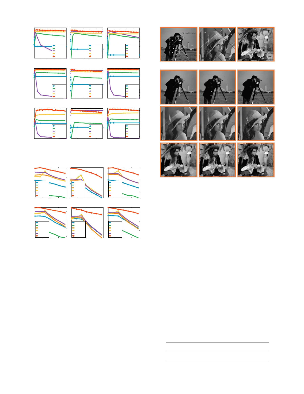
IEEE TRANSACTIONS ON P A TTERN ANAL YSIS AND MACHINE INTELLIGENCE 1 ` 0 TV : A Sparse Optimization Method f or Impulse Noise Image Restoration Ganzhao Y uan, Bernard Ghanem Abstract —T otal V ariation (TV) is an effectiv e and popular pr ior model in the ﬁeld of regularization-based image processing. This paper focuses on total v ariation for removing impulse noise in image restor ation. This type of noise frequently ar ises in data acquisition and transmission due to man y reasons, e.g. a f aulty sensor or analog-to-digital conv er ter errors. Removing this noise is an important task in image restoration. State-of-the-art methods such as Adaptive Outlier Pursuit(AOP) [59], which is based on TV with ` 02 -norm data ﬁdelity , only give sub-optimal perf ormance. In this paper , we propose a new sparse optimization method, called ` 0 T V -P ADMM, which solves the TV -based restoration problem with ` 0 -norm data ﬁdelity . T o eff ectively deal with the resulting non-conv ex non-smooth optimization problem, we ﬁrst ref ormulate it as an equivalent biconv ex Mathematical Prog ram with Equilibrium Constraints (MPEC), and then solve it using a pro ximal Alternating Direction Method of Multipliers (P ADMM). Our ` 0 T V -P ADMM method ﬁnds a desirable solution to the original ` 0 -norm optimization problem and is prov en to be convergent under mild conditions . We apply ` 0 T V -P ADMM to the problems of image denoising and deb lurr ing in the presence of impulse noise. Our e xtensive e xper iments demonstrate that ` 0 T V -P ADMM outperforms state-of-the-ar t image restoration methods. Index T erms —T otal V ar iation, Image Restoration, MPEC , ` 0 Norm Optimization, Proximal ADMM, Impulse Noise. F 1 I N T R O D U C T I O N Image restoration is an in verse problem, which aims at es- timating the original clean image u from a blurry and/or noisy observation b . Mathematically , this problem is formulated as: b = (( Ku )  ε m ) + ε a , (1) where K is a linear operator , ε m and ε a are the noise vectors, and  denotes an elementwise product. Let 1 and 0 be column vectors of all entries equal to one and zero, respectiv ely . When ε m = 1 and ε a 6 = 0 (or ε m 6 = 0 and ε a = 0 ), (1) corresponds to the additiv e (or multiplicativ e) noise model. For con venience, we adopt the vector representation for images, where a 2D M × N image is column-wise stacked into a vector u ∈ R n × 1 with n = M × N . So, for completeness, we have 1 , 0 , b , u , ε a , ε m ∈ R n , and K ∈ R n × n . Before proceeding, we present an image restoration example on the well-kno wn ‘barbara’ image using our proposed method for solving impulse noise remov al in Figure 1. In general image restoration problems, K represents a certain linear operator , e.g. con volution, wa velet transform, etc., and recov ering u from b is known as image deconv olution or image deblurring. When K is the identity operator , estimating u from b is referred to as image denoising [50]. The problem of estimating u from b is called a linear in verse problem which, for most scenarios of practical interest, is ill-posed due to the singularity and/or the ill-conditioning of K . Therefore, in order to stabilize the recovery of u , it is necessary to incorporate prior-enforcing regularization on the solution. Therefore, image restoration can be modelled globally as the following optimization problem: • Ganzhao Y uan (corr esponding author) is with School of Data and Com- puter Science, Sun Y at-sen University (SYSU), China, and also with Ke y Laboratory of Machine Intellig ence and Advanced Computing, Ministry of Education, China. E-mail: yuanganzhao@gmail.com. • Bernar d Ghanem is with V isual Computing Center , King Abdullah Uni- versity of Science and T echnology (KA UST), Saudi Arabia. E-mail: bernar d.ghanem@kaust.edu.sa. Figure 1: An example of an image recovery result using our pro- posed ` 0 TV -P ADMM method. Left column: corrupted image. Middle column: recov ered image. Right column: absolute residual between these two images. min u ` ( Ku , b ) + λ Ω( ∇ x u , ∇ y u ) , (2) where ` ( Ku , b ) measures the data ﬁdelity between Ku and the observation b , ∇ x ∈ R n × n and ∇ y ∈ R n × n are two suitable linear transformation matrices such that ∇ x u ∈ R n and ∇ y u ∈ R n compute the discrete gradients of the image u along the x -axis and y -axis, respectively 1 , Ω( ∇ x u , ∇ y u ) is the regularizer on ∇ x u and ∇ y u , and λ is a positiv e parameter used to balance the two terms for minimization. Apart from regularization, other prior information such as bound constraints [5], [70] or hard constraints 1. In practice, one does not need to compute and store the matrices ∇ x and ∇ y explicitly . Since the adjoint of the gradient operator ∇ is the negati ve div ergence operator − div, i.e., h r , ∇ x u i = h− div x r , u i , h s , ∇ y u i = h− div y s , u i for any r , s ∈ R n , the inner product between vectors can be ev aluated efﬁciently . Fore more details on the computation of ∇ and div operators, please refer to [4], [14], [51]. IEEE TRANSACTIONS ON P A TTERN ANAL YSIS AND MACHINE INTELLIGENCE 2 T able 1: Data Fidelity Models Data Fidelity Function Noise and References ` 2 ( Ku , b ) = k Ku − b k 2 2 add. Gaussian noise [14], [47] ` 1 ( Ku , b ) = k Ku − b k 1 add. Laplace noise [23], [60] ` ∞ ( Ku , b ) = k Ku − b k ∞ add. uniform noise [22], [51] ` p ( Ku , b ) = h Ku − b  log( Ku ) , 1 i mul. Poisson noise [36], [49] ` g ( Ku , b ) = h log( Ku ) + b  1 Ku , 1 i mul. Gamma noise [3], [53] ` r ( Ku , b ) = h log( Ku ) + b  b  1 2Ku , 1 i mul. Rayleigh noise [2], [48] ` 02 ( Ku , b ) = k Ku − b + z k 2 2 , s.t. k z k 0 ≤ k mixed Gaussian impulse noise [59] ` 0 ( Ku , b ) = k Ku − b k 0 add./mul. impulse noise [ours] can be incorporated into the general optimization framew ork in (2). 1.1 Related W ork This subsection presents a brief revie w of existing TV methods, from the viewpoint of data ﬁdelity models, regularization models and optimization algorithms. Data Fidelity Models: The ﬁdelity function ` ( · , · ) in (2) usually penalizes the difference between Ku and b by using different norms/div ergences. Its form depends on the assumed distribution of the noise model. Some typical noise models and their corre- sponding ﬁdelity terms are listed in T able 1. The classical TV model [47] only considers TV minimization inv olving the squared ` 2 -norm ﬁdelity term for recovering images corrupted by additiv e Gaussian noise. Howe ver , this model is far from optimal when the noise is not Gaussian. Other works [23], [60] extend classical TV to use the ` 1 -norm in the ﬁdelity term. Since the ` 1 -norm ﬁdelity term coincides with the probability density function of Laplace distrib ution, it is suitable for image restoration in the presence of Laplace noise. Moreover , additive uniform noise [22], [51], multiplicativ e Poisson noise [36], and multiplicativ e Gamma noise [53] have been considered in the literature. Some extensions hav e been made to deal with mixed Rayleigh impulse noise and mixed Poisson impulse noise in [2]. Recently , a sparse noise model using an ` 02 -norm for data ﬁdelity has been inv estigated in [59] to remove impulse and mixed Gaussian impulse noise. In this paper , we consider ` 0 -norm data ﬁdelity and show that it is particularly suitable for reconstructing images corrupted with additiv e/multiplicativ e 2 impulse noise. Regularization Models: Se veral regularization models hav e been studied in the literature (see T able 2). The Tikhono v-like reg- ularization [1] function Ω tik is quadratic and smooth, therefore it is relativ ely inexpensi ve to minimize with ﬁrst-order smooth optimization methods. Ho wever , since this method tends to ov erly smooth images, it often erodes strong edges and texture details. T o address this issue, the total v ariation (TV) regularizer was proposed by Rudin, Osher and F atemi in [47] for image denoising. Sev eral other variants of TV hav e been extensiv ely studied. The original TV norm Ω tv 2 in [47] is isotropic, while an anisotropic variation Ω tv 1 is also used. From a numerical point of view , Ω tv 2 and Ω tv 1 cannot be directly minimized since they are not differ- entiable. A popular method is to use their smooth approximation Ω stv and Ω hub (see [46] for details). V ery recently , the Potts model Ω pot [9], [29], [42], which is based on the ` 0 -norm, has receiv ed much attention. It has been shown to be particularly effecti ve for image smoothing [56] and motion deblurring [57]. 2. The impulse noise has a discrete nature (corrupted or uncorrupted), thus it can be viewed as additive noise or multiplicativ e noise. T able 2: Regularization Models Regularization Function Description and References Ω tik ( g , h ) = P n i =1 g 2 i + h 2 i Tikhono v-like [1] Ω tv 2 ( g , h ) = P n i =1 ( g 2 i + h 2 i ) 1 2 Isotropic [47], [53] Ω tv 1 ( g , h ) = P n i =1 | g i | + | h i | Anisotropic [50], [60] Ω stv ( g , h ) = P n i =1 ( g 2 i + h 2 i + ε 2 ) 1 2 smooth TV [18], [51] Ω pot ( g , h ) = P n i =1 | g i | 0 + | h i | 0 Potts model [56], [57] Ω hub ( g , h ) = P n i =1 ϕ ( g i ; h i ) , ϕ ( g i ; h i ) = ( ε k g i ; h i k 2 2 / 2; k g i ; h i k 2 ≤ 1 /ε k g i ; h i k 2 − ε/ 2; otherwise Huber-Like [46] Optimization Algorithms: The optimization problems in volved in TV -based image restoration are usually difﬁcult due to the non- differentiability of the TV norm and the high dimensionality of the image data. In the past several decades, a plethora of approaches hav e been proposed, which include PDE methods based on the Euler-Lagrange equation [47], the interior-point method [18], the semi-smooth Newton method [45], the second-order cone optimization method [31], the splitting Bregman method [32], [69], the ﬁxed-point iterative method [21], Nesterov’ s ﬁrst-order optimal method [5], [44], and alternating direction methods [20], [50], [53]. Among these methods, some solve the TV problem in its primal form [50], while others consider its dual or primal- dual forms [18], [23]. In this paper, we handle the TV problem with ` 0 -norm data ﬁdelity using a primal-dual formulation, where the resulting equality constrained optimization is solved using proximal Alternating Direction Method of Multipliers (P ADMM). It is worthwhile to note that the Penalty Decomposition Algorithm (PD A) in [39] can also solve our problem, howe ver , it lacks numerical stability . This moti vates us to design a new ` 0 -norm optimization algorithm in this paper . 1.2 Contrib utions and Organization The main contributions of this paper are two-fold. (1) ` 0 -norm data ﬁdelity is proposed to address the TV -based image restoration problem 3 . Compared with existing models, our model is particu- larly suitable for image restoration in the presence of impulse noise. (2) T o deal with the resulting NP-hard 4 ` 0 norm optimiza- tion, we propose a proximal ADMM to solve an equi valent MPEC form of the problem. A preliminary version of this paper appeared in [63]. The rest of the paper is organized as follows. Section 2 presents the motiv ation and formulation of the problem for impulse noise remov al. Section 3 presents the equiv alent MPEC problem and our proximal ADMM solution. Section 4 discusses the connection between our method and prior work. Section 5 provides extensi ve and comparativ e results in favor of our ` 0 TV method. Finally , Section 6 concludes the paper . 2 M OT I VAT I O N A N D F O R M U L AT I O N S 2.1 Motiv ation This work focuses on image restoration in the presence of impulse noise, which is very common in data acquisition and transmission due to faulty sensors or analog-to-digital con verter errors, etc. Moreov er, scratches in photos and video sequences can be also 3. W e are also aware of Ref. [19] where ` 0 -norm data ﬁdelity is considered. Howe ver , their interpretation from the MAP viewpoint is not correct. 4. The ` 0 norm problem is known to be NP-hard [43], since it is equivalent to NP-complete subset selection problems. IEEE TRANSACTIONS ON P A TTERN ANAL YSIS AND MACHINE INTELLIGENCE 3 viewed as a special type of impulse noise. Ho wev er, remo ving this kind of noise is not easy , since corrupted pixels are randomly dis- tributed in the image and the intensities at corrupted pix els are usu- ally indistinguishable from those of their neighbors. There are two main types of impulse noise in the literature [23], [35]: random- valued and salt-and-pepper impulse noise. Let [ u min , u max ] be the dynamic range of an image, where u min = 0 and u max = 1 in this paper . W e also denote the original and corrupted intensity values at position i as u i and T ( u i ) , respecti vely . Random-valued impulse noise : A certain percentage of pixels are altered to take on a uniform random number d i ∈ [ u min , u max ] : T ( u i ) = ( d i , with probability r rv ; ( Ku ) i , with probability 1 − r rv . (3) Salt-and-pepper impulse noise : A certain percentage of pixels are altered to be either u min or u max : T ( u i ) =      u min , with probability r sp / 2; u max , with probability r sp / 2; ( Ku ) i , with probability 1 − r sp . (4) The abov e deﬁnition means that impulse noise corrupts a portion of pixels in the image while keeping other pixels unaffected. Ex- pectation maximization could be used to ﬁnd the MAP estimate of u by maximizing the conditional posterior probability p ( u |T ( u )) , the probability that u occurs when T ( u ) is observed. By the Bayes’ theorem, we have that p ( u |T ( u )) = p ( u ) · p ( T ( u ) | u ) / p ( T ( u )) . T aking the negativ e logarithm of the above equation, the estimate is a solution of the following minimization problem: max u log p ( T ( u ) | u ) + log p ( u ) . (5) W e now focus on the two terms in (5). (i) The expression p ( T ( u ) | u ) can be viewed as a ﬁdelity term measuring the dis- crepancy between the estimate u and the noisy image T ( u ) . The choice of the likelihood p ( T ( u ) | u ) depends upon the property of noise. From the deﬁnition of impulse noise given abov e, we have that p ( T ( u ) | u ) = 1 − r = 1 − kT ( u ) − b k 0 /n, where r is the noise density lev el as deﬁned in (3) and (4) and k · k 0 counts the number of non-zero elements in a vector . (ii) The term p ( u ) in (5) is used to regularize a solution that has a low probability . W e use a prior which has the Gibbs form: p ( u ) = 1 ϑ exp( − E ( u )) with E ( u ) = σ · Ω tv ( ∇ x u , ∇ y u ) . Here, E ( u ) is the TV prior energy functional, ϑ is a normalization factor such that the TV prior is a probability , and σ is the free parameter of the Gibbs measure. Replacing p ( T ( u ) | u ) and p ( u ) into (5) and ignoring a constant, we obtain the following ` 0 T V model: min u k Ku − b k 0 + λ P n i =1 h | ( ∇ x u ) i | p + | ( ∇ y u ) i | p i 1 /p , where λ is a positive number related to n , σ and r . The parameter p can be 1 (anisotropic TV) or 2 (isotropic TV), and ( ∇ x u ) i and ( ∇ y u ) i denote the i th component of the vectors ∇ x u and ∇ y u , respectiv ely . For con venience, we deﬁne ∀ x ∈ R 2 n : k x k p, 1 , P n i =1 ( | x i | p + | x n + i | p ) 1 p ; ∇ , h ∇ x ∇ y i ∈ R 2 n × n . In order to make use of more prior information, we consider the following box-constrained model: min 0 ≤ u ≤ 1 k o  ( Ku − b ) k 0 + λ k ∇ u k p, 1 , (6) where o ∈ { 0 , 1 } n is speciﬁed by the user . When o i is 0, it indicates the pixel in position i is an outlier , while when o i is 1, it indicates the pix el in position i is a potential outlier . For example, in our experiments, we set o = 1 for the random-v alued impulse noise and o i =  0 , b i = u min or u max 1 , otherwise for the salt-and- pepper impulse noise. In what follows, we focus on optimizing the general formulation in (6). 2.2 Equiv alent MPEC Reform ulations In this section, we reformulate the problem in (6) as an equiv alent MPEC from a primal-dual vie wpoint. First, we provide the varia- tional characterization of the ` 0 -norm using the following lemma. Lemma 1. F or any given w ∈ R n , it holds that k w k 0 = min 0 ≤ v ≤ 1 h 1 , 1 − v i , s.t. v  | w | = 0 , (7) and v ∗ = 1 − sign( | w | ) is the unique optimal solution of the pr oblem in (7). Her e, the standard signum function sign is applied componentwise, and sign(0) = 0 . Pr oof. The total number of zero elements in w can be computed as n − k w k 0 = max v ∈{ 0 , 1 } P n i =1 v i , s.t. v ∈ Φ , where Φ , { v | v i · | w i | = 0 , ∀ i ∈ [ n ] } . Note that when w i = 0 , v i = 1 will be achieved by maximization, when w i 6 = 0 , v i = 0 will be enforced by the constraint. Thus, v ∗ i = 1 − sign( | w i | ) . Since the objectiv e function is linear, maximization is always achiev ed at the boundaries of the feasible solution space. Thus, the constraint of v i ∈ { 0 , 1 } can be relaxed to 0 ≤ v i ≤ 1 , we hav e: k w k 0 = n − max 0 ≤ v ≤ 1 , v ∈ Φ P n i =1 v i = min 0 ≤ v ≤ 1 , v ∈ Φ h 1 , 1 − v i . The result of Lemma 1 implies that the ` 0 -norm minimization problem in (6) is equiv alent to min 0 ≤ u , v ≤ 1 h 1 , 1 − v i + λ k ∇ u k p, 1 s . t . v  | o  ( Ku − b ) | = 0 . (8) If u ∗ is a global optimal solution of (6), then ( u ∗ , 1 − sign( | Ku ∗ − b | )) is globally optimal to (8). Con versely , if ( u ∗ , 1 − sign( | Ku ∗ − b | )) is a global optimal solution of (8), then u ∗ is globally optimal to (6). Although the MPEC problem in (8) is obtained by increasing the dimension of the original ` 0 -norm problem in (6), this does not lead to additional local optimal solutions. Moreo ver , compared with (6), (8) is a non-smooth non-conv ex minimization problem and its non-conv exity is only caused by the complementarity constraint v  | o  ( Ku − b ) | = 0 . Such a variational characterization of the ` 0 -norm is proposed in [6], [7], [25], [27], [34], but it is not used to dev elop any opti- mization algorithms for ` 0 -norm problems. W e argue that, from a practical perspecti ve, improv ed solutions to (6) can be obtained by reformulating the ` 0 -norm in terms of complementarity constraints [40], [63], [64], [65], [66], [67]. In the follo wing section, we will dev elop an algorithm to solve (8) based on proximal ADMM and show that such a “lifting” technique can achieve a desirable solution of the original ` 0 -norm optimization problem. IEEE TRANSACTIONS ON P A TTERN ANAL YSIS AND MACHINE INTELLIGENCE 4 Algorithm 1 ( ` 0 T V -ADMM) A Proximal ADMM for Solving the Biconv ex MPEC Problem (8) (S.0) Choose a starting point ( u 0 , v 0 , x 0 , y 0 , ξ 0 , ζ 0 ) . Set k = 0 . Select step size γ ∈ (0 , 2) , µ > 0 , β = 1 , and L = µ + β k ∇ k 2 + β k K k 2 . (S.1) Solve the following minimization problems with D := L I − ( β ∇ T ∇ + β K T K ) and E := µ I :  u k +1 v k +1  = arg min 0 ≤ u , v ≤ 1 L ( u , v , x k , y k , ξ k , ζ k , π k ) + 1 2 k u − u k k 2 D + 1 2 k v − v k k 2 E (10)  x k +1 y k +1  = arg min x , y L ( u k +1 , v k +1 , x , y , ξ k , ζ k , π k ) (11) (S.2) Update the Lagrange multipliers: ξ k +1 = ξ k + γ β ( ∇ u k − x k ) , (12) ζ k +1 = ζ k + γ β ( Ku k − b − y k ) , (13) π k +1 = π k + γ β ( o  v k  | y k | ) . (14) (S.3) if ( k is a multiple of 30) , then β = β × √ 10 (S.4) Set k := k + 1 and then go to Step (S.1). 3 P R O P O S E D O P T I M I Z AT I O N A L G O R I T H M This section is de voted to the solution of (8). This problem is rather difﬁcult to solve, because it is neither con vex nor smooth. Our solution is based on the proximal ADM method, which iteratively updates the primal and dual v ariables of the augmented Lagrangian function of (8). First, we introduce two auxiliary vectors x ∈ R 2 n and y ∈ R n to reformulate (8) as: min 0 ≤ u , v ≤ 1 , x , y h 1 , 1 − v i + λ k x k p, 1 (9) s . t . ∇ u = x , Ku − b = y , v  o  | y | = 0 . Let L : R n × R n × R 2 n × R n × R 2 n × R n × R n → R be the augmented Lagrangian function of (9). L ( u , v , x , y , ξ , ζ , π ) := h 1 , 1 − v i + λ k x k p, 1 + h ∇ u − x , ξ i + β 2 k ∇ u − x k 2 + h Ku − b − y , ζ i + β 2 k Ku − b − y k 2 + h v  o  | y | , π i + β 2 k v  o  | y |k 2 , where ξ , ζ and π are the Lagrange multipliers associated with the constraints ∇ u = x , Ku − b = y and v  o  | y | = 0 , respectiv ely , and β > 0 is the penalty parameter . The detailed iteration steps of the proximal ADM for (9) are described in Algorithm 1. In simple terms, ADM updates are performed by optimizing for a set of primal variables at a time, while keeping all other primal and dual variables ﬁxed. The dual variables are updated by gradient ascent on the resulting dual problem. Next, we focus our attention on the solutions of the sub- problems in (10) and (11) arising in Algorithm 1. W e will show that the computation required in each iteration of Algorithm 1 is insigniﬁcant. (i) ( u , v ) -subproblem. Proximal ADM introduces a con vex prox- imal term to the objective. The speciﬁc form of D is chosen to expedite the computation of the closed form solution. The intro- duction of µ is to guarantee strongly con vexity of the subproblems. u -subproblem in (10) reduces to the following minimization problem: u k +1 = arg min 0 ≤ u ≤ 1 β 2 k ∇ u − x k + ξ k /β k 2 + β 2 k Ku − b − y k + ζ k /β k 2 + 1 2 k u − u k k 2 D . (15) After an elementary calculation, subproblem (15) can be simpli- ﬁed as u k +1 = arg min 0 ≤ u ≤ 1 1 2 k u − ( u k − g k /L ) k 2 with g k = ∇ T ξ k + K T ζ k + β ∇ T ( x k − ∇ u k ) + β K T ( b + y k − Ku k ) . Then, the solution u k of (10) has the follo wing closed form expression: u k +1 = min( 1 , max( 0 , u k − g k /L )) . Here the parameter L depends on the spectral norm of the linear matrices ∇ and K . Using the deﬁnition of ∇ and the classical ﬁnite differences that k ∇ y k ≤ 2 and k ∇ y k ≤ 2 (see [4], [14], [70]), the spectral norm of ∇ can be computed by: k ∇ k = k  ∇ x 0  +  0 ∇ y  k ≤ k  ∇ x 0  k + k  0 ∇ y  k = k ∇ x k + k ∇ y k ≤ 4 . v -subproblem in (10) reduces to the following minimization problem: v k +1 = arg min 0 ≤ v ≤ 1 1 2 P n i =1 s k i v 2 i + h v , c k i , where c k = o  π k  | y k | − 1 − µ v k , s k = β o  y k  y k + µ . Therefore, the solution v k can be computed as: v k +1 = min( 1 , max( 0 , − c k s k )) . (iii) ( x , y ) -subproblem. V ariable x in (11) is updated by solving the follo wing problem: x k +1 = arg min x ∈ R 2 n β 2 k x − h k k 2 + λ k x k p, 1 , where h k := ∇ u k +1 + ξ k /β . It is not dif ﬁcult to check that for p = 1 , x k +1 = sign  h k   max  | h k | − λ/β , 0  , and when p = 2 ,  x k +1 i x k +1 i + n  =  max(0 , 1 − λ/β k ( h k i ; h k i + n ) k )  " h k i h k i + n # V ariable y in (11) is updated by solving the following problem: y k +1 = arg min y β 2 k y − q k k 2 + β 2 k w k  | y | + π k /β k 2 , where q k = Ku k +1 − b + ζ k /β and w k = o  v k +1 . A simple computation yields that the solution y k can be computed in closed form as: y k +1 = sign ( q k )  max  0 , | q k |− π k  w k /β 1+ v k  w k  , Proximal ADM has excellent con vergence in practice. The global con vergence of ADM for con vex problems w as gi ven by He and Y uan in [20], [33] under the variation inequality framework. Howe ver , since our optimization problem in (8) is non-con ve x, the con vergence analysis for ADM needs additional conditions. By imposing some mild conditions, W en et al. [52] managed to show that the sequence generated by ADM con verges to a KKT point. Along a similar line, we establish the con vergence property of proximal ADM. Speciﬁcally , we have the following con vergence result. IEEE TRANSACTIONS ON P A TTERN ANAL YSIS AND MACHINE INTELLIGENCE 5 Theorem 1. Con vergence of Algorithm 1. Let X , ( u , v , x , y ) , Y , ( ξ , ζ , π ) and { X k , Y k } ∞ k =1 be the sequence gener ated by Algorithm 1. Assume that { Y k } ∞ k =1 is bounded and satisﬁes P ∞ k =0 k Y k +1 − Y k k 2 F < ∞ . Then any accumulation point of sequence satisﬁes the KKT conditions of (9). Pr oof. Please refer to A ppendix A . Remark 1. The condition P ∞ k =0 k Y k +1 − Y k k 2 F < ∞ holds when the multiplier does not change in two consecuti ve iterations. By the boundedness of the penalty parameter β and Eqs (12- 14), this condition also indicates that the equality constraints in (9) are satisﬁed. This assumption can be checked by measuring the violation of the equality constraints. Theorem 1 indicates that when the equality constraint holds, P ADMM conv erges to a KKT point. Though not satisfactory , it provides some assurance on the con vergence of Algorithm 1. Remark 2. T wo reasons explain the good performance of our method. (i) It targets a solution to the original problem in (6). (ii) It has monotone and self-penalized properties o wing to the complimentarity constraints brought on by the MPEC. Our method directly handles the complimentary constraints in (9) : v  o  | y | = 0 with v ≥ 0 . These constraints are the only sources of non-con vexity for the optimization problem and they characterize the optimality of the KKT solution of (6). These special properties of MPEC distinguish it from general nonlinear optimization [64], [65], [66], [67]. W e penalize the complimentary error of v  o  | y | (which is alw ays non-neg ative) and ensure that the error is decreasing in every iteration. 4 C O N N E C T I O N W I T H E X I S T I N G W O R K In this section, we discuss the connection between the proposed method ` 0 T V -P ADM and prior work. 4.1 Sparse Plus Low-Rank Matrix Decomposition Sparse plus low-rank matrix decomposition [35], [54] is be- coming a po werful tool that effecti vely corrects lar ge errors in structured data in the last decade. It aims at decomposing a giv en corrupted image B (which is of matrix form) into its sparse component ( S ) and low-rank component ( L ) by solving: min B , L k S k 0 + λ r ank ( L ) , s.t. B = L + S . Here the sparse component represents the foreground of an image which can be treated as outliers or impulse noise, while the lo w-rank component corresponds to the background, which is highly correlated. This is equiv alent to the following optimization problem: min L k B − L k 0 + λ rank ( L ) , which is also based on ` 0 -norm data ﬁdelity . While they consider the low-rank prior in their objecti ve function, we consider the T otal V ariation (TV) prior in ours. 4.2 Con vex Optimization Method ` 1 T V The goal of image restoration in the presence of impulse noise has been pursued by a number of authors (see, e.g., [23], [60]) using ` 1 T V , which can be formulated as follows: min 0 ≤ u ≤ 1 k Ku − b k 1 + λ k ∇ u k p, 1 . (16) It is generally believed that ` 1 T V is able to remove the impulse noise properly . This is because ` 1 -norm provides the tightest con vex relaxation for the ` 0 -norm over the unit ball in the sense of ` ∞ -norm. It is shown in [12] that the problem of minimizing k Ku − b k 1 is equivalent to k Ku − b k 0 with high probability under the assumptions that (i) Ku − b is sparse at the optimal solution u ∗ and (ii) K is a random Gaussian matrix and sufﬁ- ciently “incoherent” (i.e., number of rows in K is greater than its number of columns). Howe ver , these two assumptions required in [12] do not necessarily hold true for our ` 0 T V optimization problem. Speciﬁcally , when the noise level of the impulse noise is high, Ku − b may not be sparse at the optimal solution u ∗ . Moreov er, the matrix K is a square identity or ill-conditioned matrix. Generally , ` 1 T V will only lead to a sub-optimal solution. 4.3 Adaptive Outlier Pursuit Algorithm V ery recently , Y an [59] proposed the following ne w model for image restoration in the presence of impulse noise and mixed Gaussian impulse noise: min u , z χ k Ku − b − z k 2 2 + k ∇ u k p, 1 , s.t. k z k 0 ≤ k , (17) where χ > 0 is the regularization parameter . They further reformulate the problem abov e into min u , v k v  ( Ku − b ) k 2 2 + λ k ∇ u k p, 1 , s.t. 0 ≤ v ≤ 1 , h v , 1 i ≤ n − k and then solve this problem using an Adaptive Outlier Pursuit(A OP) algorithm. The A OP algorithm is actually an alternating minimization method, which separates the minimization problem over u and v into two steps. By iterati vely restoring the images and updating the set of damaged pixels, it is shown that A OP algorithm outperforms existing state-of-the-art methods for impulse noise denoising, by a large margin. Despite the merits of the A OP algorithm, we must point out that it incurs three drawbacks, which are unappealing in practice. First, the formulation in (17) is only suitable for mixed Gaussian impulse noise, i.e. it produces a sub-optimal solution when the observed image is corrupted by pure impulse noise. (ii) Secondly , A OP is a multiple-stage algorithm. Since the minimization sub- problem ov er u 5 needs to be solved exactly in each stage, the algorithm may suffer from slow con vergence. (iii) As a by-product of (i), A OP inevitably introduces an additional parameter (that speciﬁes the Gaussian noise le vel), which is not necessarily readily av ailable in practical impulse denoising problems. In contrast, our proposed ` 0 TV method is free from these problems. Speciﬁcally , (i) as hav e been analyzed in Section 2, i.e. our ` 0 -norm model is optimal for impulse noise remov al. Thus, our method is expected to produce higher quality image restorations, as seen in our results. (ii) Secondly , we have integrated ` 0 - norm minimization into a uniﬁed proximal ADM optimization framew ork, it is thus expected to be faster than the multiple stage approach of A OP . (iii) Lastly , while the optimization problem in (17) contains two parameters, our model only contains one single parameter . 4.4 Other ` 0 -Norm Optimization T echniques Actually , the optimization technique for the ` 0 -norm regulariza- tion problem is the key to removing impulse noise. Howe ver , existing solutions are not appealing. The ` 0 -norm problem can be reformulated as a 0 - 1 mixed integer programming [8]problem which can be solv ed by a tailored branch-and-bound algorithm but it in volv es high computational complexity . The simple projection methods are inapplicable to our model since they assume the 5. It actually reduces to the ` 2 T V optimization problem. IEEE TRANSACTIONS ON P A TTERN ANAL YSIS AND MACHINE INTELLIGENCE 6 objectiv e function is smooth. Similar to the ` 1 relaxation, the con vex methods such as k -support norm relaxation [41], k -largest norm relaxation [62], QCQP and SDP relaxations [15] only pro- vide loose approximation of the original problem. The non-con vex methods such as Schatten ` p norm [28], [37], re-weighted ` 1 norm [13], ` 1-2 norm DC (dif ference of con vex) approximation [61], the Smoothly Clipped Absolute De viation (SCAD) penalty method [68], the Minimax Concav e Plus (MCP) penalty method [26] only produce sub-optimal results since they gi ve approximate solutions for the ` 0 T V problem or incur high computational overhead. W e take ` p norm approximation method for example and it may suffer two issues. First, it in volves an additional hyper - parameter p which may not be appealing in practice. Second, the ` p regularized norm problem for general p could be difﬁcult to solve. This includes the iterativ e re-weighted least square method [38] and proximal point method. The former approximates k x k p p by P n i =1 ( x 2 i +  ) p/ 2 with a small parameter  and solves the resulting re-weighted least squares sub-problem which reduces to a weighted ` 2 T V problem. The latter needs to ev aluate a relativ ely expensi ve proximal operator Π( a ) = min x 1 2 k x − a k 2 2 + λ k x k p p in general, except that it has a closed form solution for some special v alues such as p = 1 2 and p = 2 3 [58]. Recently , Lu et al. propose a Penalty Decomposition Al- gorithm (PD A) for solving the ` 0 -norm optimization algorithm [39]. As has been remarked in [39], direct ADM on the ` 0 norm problem can also be used for solving ` 0 T V minimization simply by replacing the quadratic penalty functions in the PDA by augmented Lagrangian functions. Nevertheless, as observed in our preliminary experiments and theirs, the practical performance of direct ADM is worse than that of PDA. Actually , in our experiments, we found PDA is unstable. The penalty function can reach very large values ( ≥ 10 8 ) , and the solution can be degenerate when the minimization problem of the augmented Lagrangian function in each iteration is not exactly solved. This motiv ates us to design a new ` 0 -norm optimization algorithm in this paper . W e consider a proximal ADM algorithm to the MPEC formulation of ` 0 -norm since it has a primal- dual interpretation. Extensive experiments have demonstrated that proximal ADM for solving the “lifting” MPEC formulation for ` 0 T V produces better image restoration qualities. 5 E X P E R I M E N TA L V A L I DAT I O N In this section, we provide empirical validation for our proposed ` 0 T V -P ADMM method by conducting extensi ve image denoising experiments and performing a thorough comparati ve analysis with the state-of-the-art. In our experiments, we use 5 well-known test images of size 512 × 512 . All code is implemented in MA TLAB using a 3.20GHz CPU and 8GB RAM. Since past studies [11], [21] have shown that the isotropic TV model performs better than the anisotropic one, we choose p = 2 as the order of the TV norm here. In our experiments, we apply the following algorithms: (i) BM3D is an image denoising strategy based on an enhanced sparse representation in transform-domain. The enhancement of the sparsity is achieved by grouping similar 2D image blocks into 3D data arrays [24]. (ii) MFM , Median Filter Methods. W e utilize adaptive median ﬁltering to remove salt-and-pepper impulse noise and adapti ve center-weighted median ﬁltering to remo ve random-v alued im- pulse noise. (iii) ` 1 T V -SBM , the Split Bregman Method (SBM) of [32], which has been implemented in [30]. W e use this conv ex optimization method as our baseline implementation. (iv) TSM , the T wo Stage Method [10], [16], [17]. The method ﬁrst detects the damaged pixels by MFM and then solves the TV image inpainting problem. (v) ` p T V -ADMM (direct) . W e directly use ADMM (Alternating Direction Method of Multipliers) to solve the non-smooth non- con vex ` p problem with proximal operator being computed ana- lytically . W e only consider p = 1 2 in our experiments [58]. (vi) ` 02 T V -A OP , the Adapti ve Outlier Pursuit (A OP) method described in [59]. W e use the implementation provided by the author . Here, we note that A OP iterativ ely calls the ` 1 T V - S B M procedure, mentioned above. (vii) ` 0 T V -PDA , the Penalty Decomposition Algorithm (PD A) [39] for solving the ` 0 T V optimization problem in (6). (viii) ` 0 T V -P ADMM , the proximal ADMM described in Algo- rithm 1 for solving the ` 0 T V optimization problem in (6). W e set the relaxation parameter to 1.618 and the strongly con ve x parame- ter µ to 0 . 01 . All MA TLAB codes to reproduce the e xperiments of this paper are available online at the authors’ research webpages. 5.1 Experiment Setup For the denoising and deblurring test, we use the following strategies to generate artiﬁcial noisy images. (a) Denoising problem . W e corrupt the original image by inject- ing random-value, salt-and-pepper noise, and mixed noise (half random-value and half salt-and-pepper) with dif ferent densities (10% to 90%) to the images. (b) Deblurring problem . Although blurring kernel estimation has been pursued by many studies (e.g. [55]), here we assume that the blurring kernel is known beforehand. W e blur the original images with a 9 × 9 Gaussian blurring kernel and add impulse noise with different densities (10% to 90%). W e use the following MA TLAB scripts to generate a blurring kernel of radius r ( r is set to 7 in the experiments): [x,y] = meshgrid ( − r:r, − r:r) , K=double(x. ˆ 2 + y . ˆ 2 < = r . ˆ 2) , P=K/sum(K(:)) . (18) W e run all the previously mentioned algorithms on the gen- erated noisy and blurry images. For ` 02 T V -A OP , we adapt the author’ s image denoising implementation to the image deblurring setting. Since both BM3D and Median Filter Methods (MFM) are not con venient to solve the deblurring problems, we do not test them in the deblurring problem. W e terminate ` 0 T V -P ADMM whenev er k ∇ u k − x k k 2 ≤ 1 255 and k Ku k − b − y k k 2 ≤ 1 255 and k o  v k  | y k |k 2 ≤ 1 255 . For ` p T V -P ADMM, ` 0 T V -PDA, and ` 0 T V -P ADMM, we use the same stopping criterion to terminate the optimization. F or ` 1 T V -SBM and ` 02 T V -A OP, we adopt the default stopping conditions provided by the authors. For the regularization parameter λ , we swept over { 0 . 1 , 0 . 6 , 1 . 1 , ..., 9 . 6 } . For the re gularization parameter χ in ` 02 T V -A OP, we swept over { 10 , 50 , 100 , 500 , 1000 , 5000 , 10000 , 50000 } and set k to the number of corrupted pixels. IEEE TRANSACTIONS ON P A TTERN ANAL YSIS AND MACHINE INTELLIGENCE 7 0 40 80 120 160 200 240 1.8e+5 2.5e+5 3.1e+5 3.8e+5 4.4e+5 Objective Iter ati on on Image Denoi si ng Probl em 8.2e+1 8.6e+1 9.0e+1 9.4e+1 9.8e+1 SNR 0 V alue 0 50 100 150 200 250 300 7.7e+4 8.8e+4 1.0e+5 1.1e+5 1.2e+5 Objective Iter ati on on Image Debl urri n g P robl em 8.0e+1 8.5e+1 9.0e+1 9.5e+1 9.9e+1 SNR 0 V alue Figure 2: Asymptotic behavior for optimizing (6) to denoise and deblur the corrupted ’cameraman’ image. W e plot the v alue of the objecti ve function (solid blue line) and the SNR value (dashed red line) against the number of optimization iterations. At speciﬁc iterations (i.e. 1, 10, 20, 40, 80, and 160), we also sho w the denoised and deblurred image. Clearly , the corrupting noise is being effecti vely remov ed throughout the optimization process. T o ev aluate these methods, we compute their Signal-to-Noise Ratios (SNRs). Since the corrupted pix els follow a Bernoulli- like distribution, it is generally hard to measure the data ﬁdelity between the original images and the recov ered images. Therefore, we consider three ways to measure SNR. S N R 0 ( u ) , n − k u 0 − u k 0 -  n − k u 0 − u 0 k 0 -  × 100 , S N R 1 ( u ) , 10 log 10 k u 0 − ¯ u k 1 k u − ¯ u k 1 , S N R 2 ( u ) , 10 log 10 k u 0 − ¯ u k 2 2 k u − ¯ u k 2 2 , where u 0 is the original clean image and ¯ u is the mean intensity value of u 0 , and k · k 0 -  is the soft ` 0 -norm which counts the number of elements whose magnitude is greater than a threshold  . W e adopt  = 20 255 in our experiments. 5.2 Con vergence of ` 0 T V -P ADMM Here, we verify the con ver gence property of our ` 0 T V -P ADMM method on denoising and deblurring problems by considering the ‘cameraman’ image subject to 30% random-valued impulse noise. W e set λ = 8 for this problem. W e record the objecti ve and SNR values for ` 0 T V -P ADMM at ev ery iteration k and plot these results in Figure 2. W e make two important observations from these results. (i) ) The objective value (or the SNR value) does not necessarily decrease (or increase) monotonically , and we attribute this to the non-con vexity of the optimization problem and the dynamic updates of the penalty factor in Algorithm 1. (ii) The objectiv e and SNR values stabilize after the 120 th iteration, which means that our algorithm has con verged, and the increase of the SNR value is negligible after the 80 th iteration. This implies that one may use a looser stopping criterion without sacriﬁcing much restoration quality . 2 4 6 8 10 10 2 L1TV−SBM LpTV−ADM L02TV−AOP L0TV−PDA L0TV−PADM (a) Random-V alue 2 4 6 8 10 10 2 L1TV−SBM LpTV−ADM L02TV−AOP L0TV−PDA L0TV−PADM (b) Salt-and-Pepper 2 4 6 8 10 10 2 L1TV−SBM LpTV−ADM L02TV−AOP L0TV−PDA L0TV−PADM (c) Mixed 2 4 6 8 10 10 1.7 10 1.8 10 1.9 L1TV−SBM LpTV−ADM L02TV−AOP L0TV−PDA L0TV−PADM (d) Random-V alue 2 4 6 8 10 10 2 L1TV−SBM LpTV−ADM L02TV−AOP L0TV−PDA L0TV−PADM (e) Salt-and-Pepper 2 4 6 8 10 10 2 L1TV−SBM LpTV−ADM L02TV−AOP L0TV−PDA L0TV−PADM (f) Mixed 2 4 6 8 10 10 1.4 10 1.5 10 1.6 10 1.7 10 1.8 L1TV−SBM LpTV−ADM L02TV−AOP L0TV−PDA L0TV−PADM (g) Random-V alue 2 4 6 8 10 10 1.3 10 1.5 10 1.7 10 1.9 L1TV−SBM LpTV−ADM L02TV−AOP L0TV−PDA L0TV−PADM (h) Salt-and-Pepper 2 4 6 8 10 10 1.4 10 1.6 10 1.8 L1TV−SBM LpTV−ADM L02TV−AOP L0TV−PDA L0TV−PADM (i) Mixed Figure 3: Image denoising with varying the tuning parameter λ in (6) on ‘cameraman’ image. First row: noise lev el = 50%. Second row: noise level = 70%. Third row: noise le vel = 90%. 5.3 General Ima g e Denoising Pr oblems In this subsection, we compare the performance of all 6 methods on general denoising problems. T able 3 sho ws image reco very results when random-value or salt-and-pepper or mixed impulse noise is added. Figure 3 sho ws image recov ery results with v arying the regularization parameter λ . For ` 02 T V model in (17), the parameter χ is scaled to the range [0 , 10] for better visualization. W e make the following interesting observations. (i) The ` 02 T V - A OP method greatly improves upon ` 1 T V -SBM, MFM and TSM, IEEE TRANSACTIONS ON P A TTERN ANAL YSIS AND MACHINE INTELLIGENCE 8 T able 3: General denoising problems. The results separated by ‘/’ are S N R 0 , S N R 1 and S N R 2 , respectively . The 1 st , 2 nd , and 3 rd best results are colored with red , blue and green , respectively . Img. Alg. BM3D ` 1 T V - S B M M F M T S M ` 02 T V - AOP ` P T V - P ADM M ` 0 T V - P D A ` 0 T V - P ADM Random-V alue Impulse Noise walkbridge+10% 93/7.1/11.0 95 /12.3/15.6 92/7.7/12.3 95 /11.8/12.9 96 / 12.8 / 16.6 95 /12.1/13.8 97 / 14.1 / 16.9 97 / 13.8 / 15.9 walkbridge+30% 76/3.7/7.1 89 / 8.6 /11.0 82/6.1/10.3 85 /5.8/7.8 89 /8.4/ 12.1 89 /7.8/11.5 91 / 9.6 / 12.8 91 / 9.5 / 11.9 walkbridge+50% 59/2.2/4.3 76/ 4.9 /5.7 67/4.1/7.0 69/2.7/4.8 76/ 5.4 /8.1 79 / 5.4 / 8.7 84 / 7.0 / 10.1 85 / 7.0 / 9.2 walkbridge+70% 42/1.0/1.9 56/2.0/1.7 45/2.0/3.3 50/1.3/2.2 53/2.5/4.0 59 / 3.0 / 5.0 65 / 4.0 / 6.2 76 / 5.1 / 7.0 walkbridge+90% 26/-0.1/-0.1 32 /-0.2/-1.1 28/0.3/0.5 30/0.0/-0.0 31/ 0.4 / 0.8 30/ 0.4 / 0.8 34 / 0.7 / 1.3 57 / 2.7 / 3.9 pepper+10% 67/5.0/9.9 99 / 19.1 / 21.5 99 /15.0/ 22.2 97 /13.5/15.8 74/5.4/11.3 99 /13.6/20.3 100 / 20.2 / 24.6 99 / 18.0 /21.0 pepper+30% 55/3.7/7.0 96 / 12.3 /13.6 96 /11.4/16.3 87 /6.3/9.5 72/5.2/10.7 98 /12.0/ 16.8 98 / 15.1 / 19.7 98 / 14.6 / 18.3 pepper+50% 44/2.4/4.5 85 /6.7/6.7 85 /7.0/9.7 71/3.5/5.5 65/4.5/8.9 94 / 9.7 / 13.1 96 / 11.8 / 15.7 96 / 11.6 / 14.4 pepper+70% 33/1.2/2.1 63/2.8/2.1 59/3.1/4.4 52/1.6/2.4 51/2.7/4.7 79 / 5.2 / 6.2 84 / 6.8 / 8.9 93 / 9.0 / 11.4 pepper+90% 24/0.2/0.1 35 /0.1/-1.0 30/0.6/0.6 31/0.3/0.1 28/0.7/ 1.1 35 / 0.9 /1.0 39 / 1.3 / 1.7 76 / 4.2 / 4.8 mandrill+10% 74/3.3/6.0 89/8.1/9.0 92 /6.9/6.9 93 / 9.6 / 9.6 84/3.7/7.4 93 / 9.6 / 9.6 95 / 11.1 / 11.5 95 / 10.8 / 10.3 mandrill+30% 63/2.0/3.6 83/ 5.9 / 6.6 76/3.8/5.9 83/4.7/4.9 73/3.0/5.5 85 /5.8/ 6.8 87 / 6.8 / 7.4 86 / 6.4 /6.5 mandrill+50% 50/1.1/2.2 73/ 3.6 /3.7 65/2.9/ 4.6 69/2.0/3.4 61/2.2/4.0 74 / 3.6 / 5.0 77 / 4.6 / 5.6 78 / 4.4 / 4.6 mandrill+70% 36/0.4/0.8 57/1.4/0.6 51/1.5/2.4 52/0.9/1.5 47/1.2/2.2 62 / 2.3 / 3.4 64 / 2.9 / 3.9 70 / 3.1 / 3.5 mandrill+90% 28/-0.3/-0.6 36/-0.6/-1.9 37/0.2/0.4 34/-0.1/-0.4 33/0.1/0.3 39 / 0.5 / 0.9 42 / 0.8 / 1.2 58 / 1.9 / 2.5 lake+10% 92/6.9/12.5 98 / 16.9 / 21.3 96 /11.3/17.7 97 /14.0/15.0 97 /8.7/16.1 98 /14.3/19.2 98 / 17.2 / 21.1 98 / 16.7 / 19.5 lake+30% 75/4.3/8.1 93 / 11.3 /13.9 91/9.3/ 14.4 86/7.1/10.0 92 /7.9/13.9 95 /10.5/ 15.0 95 / 12.7 / 16.7 95 / 12.0 /14.3 lake+50% 58/2.6/4.9 79/6.5/7.2 71/5.9/9.4 69/3.7/5.9 78/6.2/10.2 88 / 8.3 / 11.7 91 / 10.0 / 13.7 90 / 9.5 / 11.5 lake+70% 41/1.3/2.3 54/2.9/2.6 42/2.5/4.1 47/1.8/2.8 43/2.8/4.6 60 / 4.7 / 7.0 68 / 5.8 / 8.6 84 / 7.4 / 9.0 lake+90% 24/0.3/0.3 26 /0.5/-0.4 25 /0.6/0.8 26 /0.5/0.4 24/0.6/1.0 13/ 0.7 / 1.1 26 / 1.1 / 1.7 62 / 4.2 / 5.3 jetplane+10% 39 /2.5/6.1 99 / 17.5 / 21.0 98 /11.5/17.5 98 /12.8/13.3 39 /3.4/8.3 99 /13.1/ 19.1 99 / 17.0 / 20.0 98 / 15.6 /17.0 jetplane+30% 32/0.7/2.6 95 /10.3/11.5 94 /9.0/ 13.3 87/5.0/7.3 38/3.2/7.5 97 / 10.4 / 15.0 97 / 12.4 / 15.7 97 / 11.5 /12.6 jetplane+50% 27/-0.6/-0.1 80 /4.5/4.0 75/4.2/6.7 69/1.5/2.8 34/2.4/5.2 92 / 7.9 / 10.6 94 / 9.3 / 12.2 94 / 9.0 / 10.0 jetplane+70% 22/-1.7/-2.4 53/0.6/-0.7 42/0.2/0.9 47/-0.5/-0.5 23/-0.6/-0.3 67 / 3.2 / 4.8 74 / 4.4 / 6.4 90 / 6.7 / 7.4 jetplane+90% 18/-2.5/-4.1 25 /-1.8/-3.6 25 /-1.7/-2.5 26 /-1.8/-2.9 18/-2.3/-3.4 14/ -1.6 / -2.2 26 / -1.2 / -1.5 74 / 3.4 / 3.7 Salt-and-Pepper Impulse Noise walkbridge+10% 90/5.4/9.9 96 /12.9/17.3 90/7.6/12.4 98 /15.8/19.9 98 / 16.3 / 20.7 98 /15.8/19.9 99 / 17.2 / 22.7 99 / 17.5 / 23.2 walkbridge+30% 71/3.0/4.5 94 /10.4/14.3 83/6.3/9.8 96 / 11.7 / 16.4 94 /10.5/15.2 96 / 11.7 / 16.4 96 / 12.0 / 17.1 97 / 12.3 / 17.5 walkbridge+50% 51/-0.1/-1.7 89 /8.1/11.4 71/4.0/5.4 92 / 9.3 / 14.0 88/7.8/11.8 92 / 9.3 / 13.9 92 / 9.2 /13.8 93 / 9.5 / 14.3 walkbridge+70% 32/-2.0/-4.6 82 /6.1/8.7 49/1.4/2.7 87 / 7.3 / 11.5 69/4.4/6.9 87 / 7.3 / 11.5 85 / 6.9 / 11.0 87 / 7.4 / 11.6 walkbridge+90% 15/-3.2/-6.2 67 / 3.7 /5.1 26/0.2/0.6 73 / 4.8 / 7.8 36/0.9/1.6 73 / 4.8 / 7.7 56/ 3.3 / 5.8 74 / 4.8 / 7.8 pepper+10% 68/4.9/9.6 99 /14.8/20.1 99 /15.0/21.8 100 / 20.5 / 24.9 74 /5.4/11.4 100 / 20.5 / 24.9 100 / 23.2 / 30.5 100 / 23.9 / 31.0 pepper+30% 52/3.1/4.8 98 /14.6/18.3 95/10.8/13.6 99 / 16.8 / 22.9 73/5.4/11.2 99 / 16.8 / 22.9 99 / 17.7 / 24.8 100 / 18.5 / 25.6 pepper+50% 38/0.3/-1.1 97 /12.9/16.1 84 /6.1/7.0 99 / 14.9 / 21.5 71/5.2/10.6 99 / 14.8 / 21.5 99 /14.5/ 21.1 99 / 15.4 / 22.4 pepper+70% 25/-1.5/-3.9 95 /10.6/13.3 57/2.1/3.4 98 / 12.5 / 18.5 61/3.9/7.4 98 / 12.5 / 18.5 96 / 11.4 / 16.9 98 / 12.7 / 18.7 pepper+90% 14/-2.7/-5.5 89 / 7.2 /8.5 27/0.4/0.6 93 / 8.8 / 12.7 32/1.2/1.9 93 / 8.8 / 12.5 75 /4.8/7.9 93 / 9.0 / 12.9 mandrill+10% 77/2.7/4.9 93 /9.8/11.3 90/4.5/6.9 97 / 13.1 / 14.3 87/4.2/9.2 97 / 13.1 / 14.3 98 / 14.4 / 17.1 98 / 14.5 / 17.2 mandrill+30% 61/1.5/2.3 90 /7.8/9.0 75/4.0/5.9 92 / 8.9 / 10.7 79/3.6/7.2 92 / 8.9 / 10.7 93 / 9.3 / 11.8 93 / 9.4 / 11.9 mandrill+50% 44/-0.9/-2.8 84 /5.7/ 6.6 67/2.7/3.3 87 / 6.6 / 8.5 68/2.8/5.2 87 / 6.6 / 8.5 87 / 6.7 / 8.8 88 / 6.8 / 8.8 mandrill+70% 27/-2.7/-5.6 76 / 3.8 / 4.3 48/1.1/1.9 80 / 4.9 / 6.5 54/2.0/3.6 80 / 4.9 / 6.5 79 / 4.8 / 6.6 80 / 4.9 / 6.5 mandrill+90% 10/-3.8/-7.2 63 / 2.0 /1.9 36/0.3/0.6 69 / 3.1 / 4.3 35/0.4/0.8 69 / 3.1 / 4.3 59 / 2.4 / 3.8 69 / 3.1 / 4.4 lake+10% 91/6.6/11.9 99 /16.4/22.9 96 /11.3/17.6 99 / 19.6 / 25.9 99 /9.0/17.2 99 / 19.6 /25.7 100 / 20.3 / 27.5 100 / 20.6 / 27.9 lake+30% 71/3.9/5.6 97 /13.6/18.7 90/9.1/12.8 98 / 15.0 / 21.4 97 /8.6/16.0 98 / 15.0 /21.3 98 / 15.1 / 21.7 99 / 15.4 / 22.3 lake+50% 52/1.2/-0.4 94 /11.2/15.3 76/5.7/6.8 97 / 12.5 / 18.3 91/7.7/13.6 97 / 12.5 / 18.2 96 / 12.2 /17.9 97 / 12.7 / 18.6 lake+70% 33/-0.5/-3.0 90/ 9.0 / 12.1 52/2.4/3.7 93 / 10.4 / 15.2 63/5.0/8.2 93 / 10.4 / 15.2 91 / 9.7 / 14.4 94 / 10.4 / 15.2 lake+90% 18/-1.6/-4.5 80 / 6.2 / 7.5 26/0.5/0.9 84 / 7.3 / 10.1 25/1.1/1.9 83 / 7.3 / 10.1 51/4.3/7.3 84 / 7.4 / 10.2 jetplane+10% 49 /2.5/6.0 100 /17.0/23.4 98 /11.6/17.3 100 / 20.4 / 26.8 39/3.4/8.5 100 / 20.4 / 26.8 100 / 20.7 / 28.0 100 / 21.3 / 29.2 jetplane+30% 39/0.6/1.2 98 /13.6/17.9 93 /8.3/10.4 99 / 15.5 / 21.9 40/3.4/8.3 99 / 15.5 / 21.9 99 / 15.3 / 21.6 99 / 15.9 / 22.7 jetplane+50% 33/-1.4/-4.1 96 /10.9/14.1 79 /4.0/5.1 98 / 12.7 / 18.4 39/3.1/7.2 98 / 12.7 / 18.4 98 / 12.1 / 17.3 98 / 12.9 / 18.5 jetplane+70% 30/-2.8/-6.4 93 /8.5/ 10.5 53/0.3/1.2 96 / 10.2 / 14.6 32/1.2/3.0 96 / 10.2 / 14.6 94 / 9.2 / 13.3 96 / 10.3 / 14.6 jetplane+90% 28/-3.7/-7.9 87 / 5.6 / 6.0 26/-1.7/-2.1 89 / 6.6 / 8.6 29/-1.9/-2.8 89 / 6.6 / 8.6 54 /2.4/4.8 89 / 6.8 / 8.7 Mixed Impulse Noise (Half Random-V alue Noise and Half Salt-and-Pepper Noise) walkbridge+10% 91/6.1/10.1 93 /10.6/14.7 91/7.5/12.3 96 / 12.6 /13.3 96 /12.5/ 16.0 96 / 12.6 /13.3 98 / 14.8 / 17.8 98 / 15.1 / 17.9 walkbridge+30% 73/3.6/6.7 90 / 8.4 /11.8 83/6.3/10.3 88/6.6/8.3 89/ 8.6 / 12.2 92 / 8.6 / 12.2 93 / 10.2 / 13.5 93 / 10.2 / 12.9 walkbridge+50% 55/1.5/1.9 81/ 5.7 /7.0 70/4.3/6.8 76/3.5/5.7 78/ 5.7 /8.7 85 / 6.3 / 10.0 86 / 7.6 / 10.8 87 / 7.6 / 10.1 walkbridge+70% 37/-0.5/-1.8 63/2.4/1.9 50/2.0/2.9 58/1.9/3.2 56/2.8/ 4.9 72 / 4.4 / 7.2 74 / 5.1 / 7.9 80 / 5.7 / 7.9 walkbridge+90% 21/-1.9/-4.0 34/-0.6/-2.1 30/0.1/0.4 34/0.3/0.5 31/0.6/1.3 38 / 1.2 / 2.0 40 / 1.3 / 2.3 63 / 3.3 / 4.9 pepper+10% 68/5.0/9.7 98 /13.9/19.5 99 / 15.0 / 22.0 98 /14.3/16.0 74/5.4/11.3 99 /14.4/19.9 100 / 21.0 / 25.6 99 / 19.9 / 23.4 pepper+30% 54/3.7/6.8 97 /12.7/16.0 96/11.4/15.4 91/7.5/10.8 72/5.3/10.8 98 / 12.8 / 18.5 99 / 15.8 / 20.7 98 / 14.9 / 18.4 pepper+50% 41/1.8/2.3 92 / 8.5 /8.6 86 /7.0/8.9 80/4.5/7.0 68/4.8/9.5 97 / 11.2 / 16.1 97 / 12.6 / 17.1 97 / 12.6 / 15.7 pepper+70% 29/-0.1/-1.2 73/3.6/2.4 62/3.0/3.6 63/2.5/3.8 54/3.3/5.9 90 / 8.1 / 10.7 92 / 9.1 / 12.5 94 / 10.1 / 12.8 pepper+90% 19/-1.4/-3.4 39/-0.2/-2.0 33/0.4/0.5 37/0.6/0.7 31/1.0/1.5 53 / 2.1 / 2.5 49 / 2.2 / 2.9 82 / 5.6 / 6.6 mandrill+10% 76/3.0/5.3 86/6.8/8.3 91 /5.5/6.8 95 /10.4/10.1 83/3.6/7.3 95 / 10.5 / 10.3 96 / 12.1 / 12.4 96 / 11.7 / 11.2 mandrill+30% 63/1.8/3.4 82/ 5.4 /6.6 74/3.9/6.0 85 /5.3/5.1 73/2.9/5.3 88 / 6.5 / 7.4 89 / 7.3 / 8.1 89 / 7.3 / 7.5 mandrill+50% 47/0.6/0.6 75/ 3.7 /4.0 67/3.0/4.4 74/2.5/3.8 61/2.2/3.9 78 / 4.4 / 5.6 80 / 5.0 / 5.9 81 / 5.0 / 5.3 mandrill+70% 32/-1.0/-2.6 60/1.3/0.2 53/1.5/1.8 58/1.3/2.1 48/1.4/2.6 68 / 2.9 / 4.2 69 / 3.3 / 4.3 73 / 3.5 / 3.9 mandrill+90% 20/-2.4/-4.9 35/-1.2/-3.3 36/0.3/0.5 37/0.2/0.1 33/0.3/0.6 46 / 1.1 / 1.8 45 / 1.0 / 1.3 62 / 2.2 / 2.8 lake+10% 91/6.8/12.0 98 /14.6/ 20.5 96/11.3/17.7 98 / 15.0 /15.5 97 /8.7/16.1 98 / 15.0 /19.4 99 / 18.0 / 22.2 99 / 17.9 / 21.2 lake+30% 73/4.3/7.6 95 / 11.7 / 15.7 91/9.3/13.7 90/8.0/10.5 92 /7.9/13.8 96 /11.0/ 16.4 96 / 13.1 / 17.2 96 / 12.8 /15.6 lake+50% 55/2.3/2.7 87 /7.9/9.0 75/6.1/8.6 78/4.8/7.2 82 /6.6/11.0 92 / 9.3 / 13.1 92 / 10.4 / 14.1 92 / 10.0 / 12.2 lake+70% 37/0.6/-0.6 66/3.7/3.1 44/2.8/3.7 58/2.6/4.1 48/3.7/6.2 82 / 7.0 / 9.8 83 / 7.7 / 10.8 87 / 7.9 / 9.4 lake+90% 22/-0.6/-2.7 34 /0.4/-1.1 20/0.6/0.7 30/0.8/1.0 24/0.8/1.5 22/ 1.5 / 2.4 33 / 2.0 / 3.1 74 / 5.3 / 6.0 jetplane+10% 44 /2.6/6.0 99 / 15.4 / 20.8 98 /11.6/17.5 99 /13.9/13.3 39/3.4/8.3 99 /13.9/ 19.3 99 / 17.6 / 20.8 99 / 16.8 / 18.5 jetplane+30% 36/0.8/2.5 97 / 11.6 / 14.2 94 /8.8/12.3 91/6.3/8.2 38/3.2/7.7 98 /11.0/ 16.6 98 / 13.1 / 16.4 98 / 12.6 /14.1 jetplane+50% 30/-0.8/-1.6 90 /6.6/6.2 79 /4.5/5.8 79 /2.8/4.2 37/2.8/6.1 95 / 9.0 / 12.7 95 / 10.0 / 13.0 95 / 9.7 / 10.7 jetplane+70% 25/-2.1/-4.5 68/1.7/-0.1 45/0.6/0.5 60/0.4/0.9 25/0.7/1.9 88 / 6.3 / 7.9 87 / 6.6 / 8.8 91 / 7.3 / 8.0 jetplane+90% 22/-3.1/-6.4 34 /-1.8/-4.4 19/-1.8/-2.4 30/-1.5/-2.3 16/-2.1/-3.0 19/ -0.8 / -0.9 32 / -0.2 / -0.1 79 / 4.2 / 4.4 by a large margin. These results are consistent with the reported results in [59]. (ii) The ` 0 T V -PDA method outperforms ` 02 T V - A OP in most test cases because it adopts the ` 0 -norm in the data ﬁdelity term. (iii) In the case of random-value impulse noise, our ` 0 T V -P ADMM method is better than ` 0 T V -PDA in S N R 0 value while it is comparable to ` 0 T V -PDA in S N R 1 and S N R 2 . On the other hand, when salt-and-pepper impulse noise is added, we ﬁnd that ` 0 T V -P ADMM outperforms ` 0 T V -PDA in most test cases. Interestingly , the performance gap between ` 0 T V -P ADMM and ` 0 T V -PDA grows larger , as the noise lev el increases. (iv) For the same noise lev el, ` 0 T V -P ADMM achie ves better recov ery performance in the presence of salt-and-pepper impulse noise than random-valued impulse noise. This is primarily due to the fact that random-valued noise can take any value between 0 and 1, thus, making it more difﬁcult to detect which pixels are corrupted. 5.4 General Ima g e Deblurring Problems In this subsection, we demonstrate the performance of all methods with their optimal regularization parameters on general deblurring problems. T able 4 shows the recovery results for random-valued impulse noise, salt-and-pepper impulse noise, and mixed impulse noise, respectiv ely . Figure 4 sho ws image recov ery results with varying the regularization parameter . W e have the following in- teresting observations. ( i ) ` 02 T V -A OP signiﬁcantly outperforms ` 1 T V -SBM, and the performance gap becomes larger as the noise lev el increases. This is because the key assumption in the ` 1 model is that K u − b is sparse at the optimal solution u ∗ . This does not hold when the noise lev el is high. ( ii ) ` 0 T V -PDA outperforms IEEE TRANSACTIONS ON P A TTERN ANAL YSIS AND MACHINE INTELLIGENCE 9 T able 4: General deblurring problems. The results separated by ‘/’ are S N R 0 , S N R 1 and S N R 2 , respectiv ely . The 1 st , 2 nd , and 3 rd best results are colored with red , blue and green , respectively . Img. Alg. Corrupted ` 1 T V - S B M T SM ` p T V - P ADM M ` 02 T V - AO P ` 0 T V - P DA ` 0 T V - P ADM Random-V alued Impulse Noise walkbridge+10% 63/2.9/3.4 74/4.8/8.6 72/4.6/8.2 77 / 5.1 / 9.2 81 / 5.6 / 10.1 76/5.0/9.0 91 / 7.0 / 13.2 walkbridge+30% 52/1.1/0.0 72/4.6/8.1 61/3.7/6.8 75 / 4.9 / 8.7 79 / 5.4 / 9.7 74/4.8/ 8.7 86 / 6.4 / 11.7 walkbridge+50% 42/-0.2/-1.9 63/3.8/6.9 46/2.4/4.6 71/4.5/8.0 75 / 4.9 / 8.6 73 / 4.7 / 8.3 84 / 6.0 / 11.0 walkbridge+70% 31/-1.2/-3.2 46/2.1/3.8 33/1.1/2.3 55/2.9/ 5.1 65 / 3.3 /4.8 69 / 4.3 / 7.7 81 / 5.6 / 10.1 walkbridge+90% 21/-2.0/-4.2 28/0.3/0.8 25/0.2/0.5 31/ 0.6 / 1.2 33 /0.4/0.6 42 / 1.7 / 3.0 67 / 3.7 / 5.8 pepper+10% 81/4.9/4.5 94 / 9.3 / 14.7 93/8.3/13.6 70/5.1/10.1 96 / 9.7 / 15.8 94 /9.0/ 14.7 99 / 11.1 / 19.8 pepper+30% 66/2.1/0.3 92/8.5/13.3 82/5.7/9.9 68/4.9/9.7 96 / 9.7 / 15.8 93 / 8.8 / 14.1 98 / 10.7 / 18.8 pepper+50% 52/0.4/-1.8 83/6.4/9.9 58/3.4/6.0 65/4.6/8.9 95 / 9.3 / 14.9 92 / 8.5 / 13.5 98 / 10.4 / 17.8 pepper+70% 37/-0.8/-3.2 58/3.1/4.7 37/1.6/2.9 52/3.0/ 5.4 82 / 5.1 / 5.4 90 / 7.8 / 12.1 97 / 9.8 / 16.4 pepper+90% 23/-1.8/-4.3 29/0.6/1.0 24/0.4/0.7 29/ 0.9 / 1.3 38 / 0.9 /0.7 54 / 2.5 / 3.5 85 / 6.1 / 7.2 mandrill+10% 59/1.6/1.3 67 /2.9/ 4.7 65/2.7/4.3 54/2.1/3.8 68 / 3.0 /4.5 68 / 3.1 / 5.0 78 / 4.3 / 7.3 mandrill+30% 50/0.0/-1.7 66/ 2.9 / 4.6 60/2.3/3.9 52/2.1/3.7 68 / 3.0 / 4.6 67 / 3.0 / 4.8 76 / 4.0 / 6.8 mandrill+50% 40/-1.1/-3.4 64/ 2.7 /4.3 50/1.6/2.9 51/2.0/3.5 68 / 2.9 / 4.5 66 / 2.9 / 4.6 73 / 3.6 / 6.0 mandrill+70% 30/-2.0/-4.7 53/1.8/3.1 40/0.9/1.7 46/1.6/2.9 64 / 2.5 / 3.6 65 / 2.7 / 4.4 70 / 3.3 / 5.4 mandrill+90% 21/-2.7/-5.6 38/0.5/ 0.9 36/0.3/0.6 34/0.4/0.7 42 / 0.6 /0.8 49 / 1.5 / 2.5 65 / 2.7 / 4.2 lake+10% 71/4.8/4.9 84 /7.6/11.6 83/7.3/11.3 83/6.7/11.3 89 / 8.6 / 13.8 84 / 7.7 / 12.1 96 / 10.0 / 17.4 lake+30% 59/2.6/1.2 81/7.1/10.8 65/5.2/8.9 80/6.4/10.7 89 / 8.5 / 13.2 83 / 7.4 / 11.6 94 / 9.5 / 15.9 lake+50% 46/1.1/-0.7 68/5.5/8.8 35/3.2/5.6 76/6.0/9.8 86 / 7.9 / 11.9 82 / 7.2 / 11.1 92 / 9.1 / 15.1 lake+70% 34/0.0/-2.1 35/2.6/4.5 22/1.6/2.9 39/3.3/ 5.6 66 / 4.3 /5.4 79 / 6.7 / 10.2 89 / 8.5 / 13.8 lake+90% 22 /-0.9/-3.1 22 /0.6/1.0 16/0.4/0.8 22 / 0.7 / 1.3 21/0.6/0.8 31 / 2.1 / 3.5 74 / 5.6 / 7.2 jetplane+10% 76/3.3/2.1 88/6.7/9.9 88/6.1/9.7 63/2.8/6.5 93 / 7.9 / 12.5 89 / 6.8 / 10.5 98 / 9.1 / 16.6 jetplane+30% 63/0.7/-1.9 86/6.2/9.1 68/3.2/6.3 66/2.7/6.2 93 / 7.8 / 12.0 88 / 6.6 / 10.0 97 / 8.8 / 15.6 jetplane+50% 49/-0.9/-3.9 74/3.9/6.6 34/0.9/2.6 55/2.5/5.6 91 / 7.0 / 9.7 87 / 6.3 / 9.4 95 / 8.4 / 14.2 jetplane+70% 36/-2.1/-5.3 37/0.3/1.3 22/-0.7/-0.3 35/-0.1/0.6 64 / 1.5 / 1.9 84 / 5.8 / 8.5 93 / 7.8 / 12.4 jetplane+90% 23 /-3.0/-6.3 23 / -1.7 / -2.3 14/-1.9/-2.5 16/-2.2/-3.3 20/ -1.7 /-2.5 30 / 0.0 / 0.6 80 / 4.5 / 5.1 Salt-and-Pepper Impulse Noise walkbridge+10% 61/2.0/0.8 73/4.8/8.5 80 / 5.6 / 10.1 76 / 5.1 / 9.1 80 / 5.6 / 10.1 76 /5.0/9.0 94 / 7.4 / 14.3 walkbridge+30% 48/-0.5/-3.2 71/4.5/7.9 79 / 5.4 / 9.7 74/4.8/8.5 79 / 5.4 / 9.7 75 / 4.9 / 8.8 92 / 7.2 / 13.7 walkbridge+50% 35/-2.1/-5.3 67/4.1/7.3 77 / 5.2 / 9.3 72/4.5/8.1 77 / 5.2 / 9.3 73 / 4.8 / 8.5 90 / 6.8 / 12.9 walkbridge+70% 22/-3.3/-6.7 53/2.8/5.2 75 / 5.0 / 8.8 61/3.5/6.4 75 / 4.9 / 8.8 71 /4.5/ 8.1 86 / 6.4 / 11.8 walkbridge+90% 8/-4.2/-7.7 31/0.6/1.0 73 / 4.7 / 8.3 34/0.9/1.7 73 / 4.7 / 8.3 59 / 3.4 / 6.3 79 / 5.4 / 9.9 pepper+10% 79/3.6/1.3 94 /8.9/14.2 96 / 9.7 / 15.8 69/5.0/10.0 96 / 9.6 / 15.8 94 /9.1/ 14.8 99 / 11.4 / 20.3 pepper+30% 62/0.2/-3.2 92/8.5/13.2 96 / 9.6 / 15.7 69/4.9/9.6 96 / 9.6 / 15.7 94 / 8.9 / 14.4 99 / 11.2 / 19.7 pepper+50% 45/-1.7/-5.4 87/7.3/11.2 95 / 9.4 / 15.4 66/4.7/9.1 95 / 9.4 / 15.4 93 / 8.6 / 13.8 99 / 10.9 / 19.1 pepper+70% 28/-3.0/-6.8 70/4.3/6.5 95 / 9.2 / 14.8 56/3.7/6.8 95 / 9.2 / 14.9 91 / 8.3 /13.0 98 / 10.3 / 18.2 pepper+90% 11/-4.1/-7.9 33/0.8/1.1 94 / 8.8 / 14.1 32/1.1/1.8 94 / 8.8 / 14.1 79 / 5.6 / 8.8 96 / 9.5 / 15.8 mandrill+10% 58/0.7/-1.3 67 / 2.9 / 4.7 67 / 2.9 /4.4 53/2.1/3.8 67 / 2.9 /4.4 68 / 3.1 / 5.0 86 / 5.2 / 9.5 mandrill+30% 45/-1.7/-5.2 65/2.8/4.4 67 / 2.9 / 4.5 52/2.1/3.6 67 / 2.9 / 4.5 68 / 3.0 / 4.9 83 / 4.9 / 8.7 mandrill+50% 32/-3.2/-7.2 64/2.6/4.2 66 / 2.8 / 4.4 51/2.0/3.5 66 / 2.8 / 4.4 67 / 3.0 / 4.7 80 / 4.5 / 7.9 mandrill+70% 19/-4.4/-8.6 56/2.0/3.3 65 / 2.7 / 4.2 48/1.8/3.1 65 / 2.7 / 4.2 66 / 2.8 / 4.5 75 / 4.0 / 6.7 mandrill+90% 7/-5.2/-9.6 39/0.5/0.8 65 / 2.7 / 4.2 35/0.5/1.0 65 / 2.7 / 4.2 60 / 2.4 / 3.9 70 / 3.3 / 5.3 lake+10% 69/3.9/2.4 83/7.4/11.4 90 / 8.7 / 13.8 82/6.6/11.2 90 / 8.7 / 13.8 85 / 7.7 / 12.1 98 / 10.3 / 18.5 lake+30% 54/1.0/-1.8 81/7.1/10.6 89 / 8.5 / 13.4 80/6.3/10.6 89 / 8.5 / 13.4 84 / 7.6 / 11.8 97 / 10.1 / 17.9 lake+50% 38/-0.7/-3.9 76/6.4/9.6 87 / 8.2 / 12.9 77/6.0/9.8 87 / 8.2 / 12.8 82 / 7.3 /11.3 96 / 9.8 / 17.0 lake+70% 23/-1.9/-5.3 49/3.9/6.3 86 / 7.9 / 12.2 56/4.4/7.3 86 / 7.9 / 12.2 81 / 7.0 / 10.7 94 / 9.3 / 15.9 lake+90% 8/-2.8/-6.4 24/0.9/1.4 83 / 7.4 / 11.2 21/1.0/1.8 84 / 7.5 / 11.1 63/5.0/8.1 88 / 8.2 / 13.3 jetplane+10% 75/2.3/-0.4 88/6.5/9.7 93 / 8.0 / 12.6 67/2.8/6.5 93 / 8.0 / 12.6 89 / 6.9 / 10.6 99 / 9.5 / 17.8 jetplane+30% 58/-0.9/-4.8 86/6.2/9.0 93 / 7.7 / 11.9 64/2.7/6.1 92 / 7.6 / 11.8 88/6.7/10.2 99 / 9.4 / 17.2 jetplane+50% 42/-2.7/-7.0 82/5.4/7.8 91 / 7.5 / 11.4 54/2.5/5.7 91 / 7.5 / 11.5 87 / 6.5 /9.7 98 / 9.0 / 16.2 jetplane+70% 25/-3.9/-8.4 48/1.9/3.8 90 / 7.1 / 10.7 39/1.2/2.9 90 / 7.1 / 10.6 86 / 6.1 /9.0 96 / 8.7 / 14.9 jetplane+90% 8/-4.9/-9.5 24/-1.3/-1.8 89 / 6.7 / 9.7 21/-1.9/-2.8 89 / 6.7 / 9.9 72 / 3.6 /6.1 92 / 7.2 / 11.8 Mixed Impulse Noise (Half Random-V alue Noise and Half Salt-and-Pepper Noise) walkbridge+10% 62/2.4/1.9 74/4.8/8.5 72/4.6/8.2 77 / 5.1 / 9.2 81 / 5.6 / 10.1 76/5.0/9.0 93 / 7.4 / 14.0 walkbridge+30% 50/0.2/-1.9 71/4.5/7.9 65/3.9/7.2 74 / 4.8 /8.6 79 / 5.4 / 9.6 74 / 4.8 / 8.7 87 / 6.5 / 12.0 walkbridge+50% 38/-1.3/-3.9 64/3.8/6.9 52/2.9/5.5 71/4.5/8.0 78 / 5.2 / 8.8 73 / 4.7 / 8.3 84 / 6.1 / 11.0 walkbridge+70% 27/-2.3/-5.3 48/2.4/4.4 38/1.6/3.2 59/3.3/6.0 74 / 4.5 / 7.1 70 / 4.4 / 7.8 81 / 5.6 / 10.1 walkbridge+90% 15/-3.2/-6.3 29/0.5/1.0 27/0.4/0.9 33/0.8/ 1.6 43 / 1.1 /1.4 50 / 2.3 / 3.7 71 / 4.3 / 7.2 pepper+10% 80/4.2/2.6 94 / 9.1 /14.5 93/8.5/13.7 69/5.1/10.0 96 / 9.7 / 15.9 94 /9.0/ 14.7 99 / 11.1 / 19.8 pepper+30% 64/1.0/-1.8 91/8.4/13.0 87/6.4/10.9 68/4.9/9.6 96 / 9.7 / 15.8 93 / 8.8 / 14.1 99 / 10.9 / 19.3 pepper+50% 49/-0.8/-3.9 84/6.7/10.2 68/4.2/7.5 66/4.7/9.1 96 / 9.4 / 15.0 92 / 8.5 / 13.5 98 / 10.5 / 18.2 pepper+70% 33/-2.1/-5.4 61/3.5/5.2 43/2.3/4.0 54/3.4/6.3 94 / 8.4 / 11.4 90 / 7.9 / 12.2 97 / 10.0 / 16.8 pepper+90% 17/-3.1/-6.4 31/0.9/1.3 27/0.7/1.2 32/1.1/ 1.8 55 / 2.0 /1.5 60 / 3.2 / 4.9 92 / 8.2 / 11.7 mandrill+10% 58/1.1/-0.2 67 / 2.9 / 4.7 65/2.7/4.3 53/2.1/3.8 67 / 2.9 /4.6 68 / 3.1 / 5.0 85 / 5.0 / 9.4 mandrill+30% 47/-0.9/-3.7 66/ 2.8 /4.5 62/2.4/4.0 52/2.1/3.7 68 / 3.0 / 4.6 67 / 3.0 / 4.8 76 / 4.0 / 6.8 mandrill+50% 36/-2.3/-5.7 64/ 2.6 / 4.2 54/1.9/3.3 51/2.0/3.4 68 / 2.9 / 4.6 66 / 2.9 / 4.6 74 / 3.7 / 6.3 mandrill+70% 25/-3.3/-7.0 54/1.9/3.2 43/1.1/2.2 47/1.7/3.1 67 / 2.8 / 4.2 65 / 2.7 / 4.4 71 / 3.4 / 5.4 mandrill+90% 14/-4.2/-8.1 38/0.4/0.7 36/0.4/0.8 35/0.5/0.9 50 / 1.3 / 1.4 48 / 1.0 / 1.1 66 / 2.8 / 4.3 lake+10% 70/4.3/3.5 83/7.5/11.5 83/7.4/11.4 82/6.6/11.3 89 / 8.6 / 13.8 84 / 7.7 / 12.1 97 / 10.0 / 17.9 lake+30% 56/1.7/-0.5 80/7.0/10.6 74/5.8/9.6 80/6.3/10.6 88 / 8.4 / 13.3 83 / 7.5 / 11.6 94 / 9.5 / 16.2 lake+50% 42/0.1/-2.6 73/6.0/9.3 45/4.0/7.0 77/6.0/9.8 88 / 8.1 / 11.8 82 / 7.2 / 11.1 92 / 9.1 / 15.1 lake+70% 29/-1.0/-4.0 40/2.9/5.1 27/2.3/4.0 51/4.1/6.8 84 / 7.4 / 10.8 79 / 6.8 / 10.3 89 / 8.5 / 13.5 lake+90% 15/-2.0/-5.0 18/0.7/1.2 17/0.7/1.3 18/0.9/ 1.6 32 / 1.4 /1.5 55 / 3.8 / 5.4 81 / 6.8 / 9.8 jetplane+10% 76/2.8/0.6 88/6.7/9.9 89 /6.4/9.8 66/2.8/6.5 93 / 7.9 / 12.5 89 / 6.8 / 10.5 98 / 9.1 / 16.6 jetplane+30% 60/-0.2/-3.6 86/6.2/8.9 79/4.1/7.5 66/2.7/6.1 93 / 7.8 / 11.8 88 / 6.6 / 9.9 97 / 8.8 / 15.6 jetplane+50% 45/-1.9/-5.7 81/5.0/7.5 44/1.9/4.2 51/2.5/5.6 91 / 7.1 / 10.3 87 / 6.4 / 9.5 95 / 8.4 / 14.1 jetplane+70% 30/-3.1/-7.1 39/0.7/2.2 25/0.0/1.0 32/0.8/2.2 89 / 6.4 / 8.4 85 / 5.9 / 8.7 93 / 7.7 / 12.2 jetplane+90% 15/-4.1/-8.2 16/-1.6/-2.1 16/-1.6/-2.0 22/-2.0/-3.0 30 / -1.1 / -1.8 56 / 2.0 / 3.1 86 / 5.8 / 7.8 ` 02 T V -A OP for high le vel ( ≥ 30% ) random-valued impulse noise. Ho wever , for salt-and-pepper impulse noise, ` 0 T V -PDA giv es worse performance than ` 02 T V -A OP in most cases. This phenomenon indicates that the Penalty Decomposition Algorithm is not stable for deblurring problems. ( iii ) By contrast, our ` 0 T V - P ADMM consistently outperforms all methods, especially when the noise level is large. W e attribute this result to the “lifting” technique that is used in our optimization algorithm. Finally , we also report the performance of all methods with sweeping the radius parameter r as in (18) over { 1 , 4 , 7 , ..., 20 } in Figure 5. W e notice that the restoration quality degenerates as the radius of the kernel increases for all methods. Howe ver , our method consistently gives the best performance. 5.5 Scratched Image Denoising Problems In this subsection, we demonstrate the superiority of the proposed ` 0 T V -P ADMM in real-world image restoration problems. Specif- ically , we corrupt the images with scratches which can be viewed as impulse noise 6 , see Figure 6. W e only consider recov ering images using ` 02 T V -A OP , ` 0 T V -PDA and ` 0 T V -P ADMM. W e show the recov ered results in Figure 7. For better visualization of the images recov ered by all methods, we also show auxiliary images c in Figure 8, which sho w the complement of the absolute residual between the recovered image u and the corrupted image b (i.e., c = { 1 − | b − u |} ). Note that when c i is approximately 6. Note that this is different from the classical image inpainting problem that assumes the mask is known. In our scratched image denoising problem, we assume the mask is unknown. IEEE TRANSACTIONS ON P A TTERN ANAL YSIS AND MACHINE INTELLIGENCE 10 2 4 6 8 10 10 2 L1TV−SBM LpTV−ADM L02TV−AOP L0TV−PDA L0TV−PADM (a) Random-V alue 2 4 6 8 10 10 2 L1TV−SBM LpTV−ADM L02TV−AOP L0TV−PDA L0TV−PADM (b) Salt-and-Pepper 2 4 6 8 10 10 2 L1TV−SBM LpTV−ADM L02TV−AOP L0TV−PDA L0TV−PADM (c) Mixed 2 4 6 8 10 10 1 10 2 L1TV−SBM LpTV−ADM L02TV−AOP L0TV−PDA L0TV−PADM (d) Random-V alue 2 4 6 8 10 10 2 L1TV−SBM LpTV−ADM L02TV−AOP L0TV−PDA L0TV−PADM (e) Salt-and-Pepper 2 4 6 8 10 10 1 10 2 L1TV−SBM LpTV−ADM L02TV−AOP L0TV−PDA L0TV−PADM (f) Mixed 2 4 6 8 10 10 1 L1TV−SBM LpTV−ADM L02TV−AOP L0TV−PDA L0TV−PADM (g) Random-V alue 2 4 6 8 10 10 2 L1TV−SBM LpTV−ADM L02TV−AOP L0TV−PDA L0TV−PADM (h) Salt-and-Pepper 2 4 6 8 10 10 1 L1TV−SBM LpTV−ADM L02TV−AOP L0TV−PDA L0TV−PADM (i) Mixed Figure 4: Image deblurring with v arying the tuning parameter λ in (6) on ‘ cameraman’ image. First row: noise level = 50%. Second row: noise level = 70%. Third row: noise le vel = 90%. 5 10 15 20 10 1.8 10 1.9 L1TV−SBM TSM LpTV−ADM L02TV−AOP L0TV−PDA L0TV−PADM (a) Random-V alue 5 10 15 20 10 2 L1TV−SBM TSM LpTV−ADM L02TV−AOP L0TV−PDA L0TV−PADM (b) Salt-and-Pepper 5 10 15 20 10 1.8 10 1.9 L1TV−SBM TSM LpTV−ADM L02TV−AOP L0TV−PDA L0TV−PADM (c) Mixed 5 10 15 20 10 1.6 10 1.7 10 1.8 10 1.9 L1TV−SBM TSM LpTV−ADM L02TV−AOP L0TV−PDA L0TV−PADM (d) Random-V alue 5 10 15 20 10 1.8 10 1.9 L1TV−SBM TSM LpTV−ADM L02TV−AOP L0TV−PDA L0TV−PADM (e) Salt-and-Pepper 5 10 15 20 10 1.7 10 1.8 10 1.9 L1TV−SBM TSM LpTV−ADM L02TV−AOP L0TV−PDA L0TV−PADM (f) Mixed Figure 5: Image deblurring with varying the radius parameter r in (18). First row: ‘cameraman’ image. Second row: ‘barbara’ image. equal to 1 , the color of the corresponding pixel at position i in the image is white. A conclusion can be drawn that our method ` 0 T V -P ADMM generates more ‘white’ images c than the other two methods, since it can identify the ‘right’ outliers in the corrupted image and mak e the correction using their neighborhood information. 5.6 Colored Ima g e Denoising Pr oblems Our proposed method can be directly extended to its color version. Since color total variation is not the main theme of this paper , we only provide a basic implementation of it. Speciﬁcally , we compute the color total variation channel-by-channel, and take a ` 1 -norm of the resulting vectors. Suppose we have RGB channels, then we have the following optimization problem: min 0 ≤ u 1 , u 2 , u 3 ≤ 1 P 3 k =1 ( k o k  ( Ku k − b k ) k 0 + λ k ∇ u k k p, 1 ) , Figure 6: Sample images in scratched image denoising problems. Figure 7: Recov ered images in scratched image denoising problems. First column: ` 02 T V -A OP , second column: ` 0 T V -PDA, third col- umn: ` 0 T V -P ADMM. where o k and u k are the prior and the solution of the k th channel. The grayscale proximal ADM algorithm in Algorithm 1 can be directly extended to solve the optimization above. W e demonstrate its applicability in colored image denoising problems in Figure 9. The regularization parameter λ is set to 8 for the three images in our experiments. 5.7 Running Time Comparisons W e provide some running time comparisons for the methods ` 1 T V -SBM, TSM, ` p T V -ADMM, ` 02 T V -A OP , ` 0 T V -PDA, and ` 0 T V -P ADMM on grayscale image ‘cameraman’ corrupted by 50% random-value impulse noise. For RGB color images, the running time is three times the amount of grayscale images since the colored image recovery problem can be decomposed into dependent subproblems. T able 5 sho ws the av erage CPU time for ﬁv e runs. Generally , our method is efﬁcient and comparable with existing solutions. This is expected since our method is an alternating optimization algorithm. T able 5: CPU time (in seconds) comparisons. First row: image denoising; second row: image deblurring. ` 1 T V - S B M T S M ` p T V - ADMM ` 02 T V - A OP ` 0 T V - PD A ` 0 T V - P ADM M 5 ± 4 6 ± 4 15 ± 4 30 ± 5 17 ± 3 14 ± 4 15 ± 8 16 ± 7 38 ± 8 62 ± 4 39 ± 7 35 ± 8 IEEE TRANSACTIONS ON P A TTERN ANAL YSIS AND MACHINE INTELLIGENCE 11 Figure 8: Absolute residual (between scratched image and recov ered image) in scratched image denoising problems. First column: ` 02 T V - A OP , second column: ` 0 T V -PDA, third column: ` 0 T V -P ADMM. (a) clean ‘lenna’ (b) corrupted ‘lenna’ (c) recovered ‘lenna’ Figure 9: Colored image denoising problems. 6 C O N C L U S I O N S In this paper , we propose a ne w method for image restoration based on total variation (TV) with ` 0 -norm data ﬁdelity , which is particularly suitable for removing impulse noise. Although the resulting optimization model is non-con vex, we design an efﬁcient and effecti ve proximal ADM method for solving the equi valent MPEC problem of the original ` 0 -norm minimization problem. Extensiv e numerical experiments indicate that the proposed ` 0 TV model signiﬁcantly outperforms the state-of-the-art in the presence of impulse noise. In particular , our proposed proximal ADM solver is more effecti ve than the penalty decomposition algorithm used for solving the ` 0 TV problem [39]. Acknowledgments. W e would lik e to thank Prof. Shaohua P an for her helpful discussions on this paper . W e also thank Prof. Ming Y an for sharing his code with us. This work was supported by the King Abdullah Univ ersity of Science and T echnology (KA UST) Ofﬁce of Sponsored Research and, in part, by the NSF-China (61772570, 61402182). R E F E R E N C E S [1] V . A. A. T ikhonov . Solution of ill-posed pr oblems . W inston, W ashington, DC, 1977. [2] M. V . Afonso and J. M. Raposo Sanches. Blind inpainting using and total variation regularization. IEEE T ransactions on Image Pr ocessing , 24(7):2239–2253, 2015. [3] G. Aubert and J.-F . Aujol. A variational approach to removing multi- plicativ e noise. SIAM J ournal on Applied Mathematics , 68(4):925–946, 2008. [4] J.-F . Aujol. Some ﬁrst-order algorithms for total v ariation based image restoration. Journal of Mathematical Imaging and V ision , 34(3):307–327, 2009. [5] A. Beck and M. T eboulle. Fast gradient-based algorithms for constrained total variation image denoising and deblurring problems. IEEE T ransac- tions on Image Pr ocessing , 18(11):2419–2434, 2009. [6] S. Bi. Study for multi-stage conv ex relaxation approach to low-rank optimization problems, phd thesis, south china university of technology . 2014. [7] S. Bi, X. Liu, and S. Pan. Exact penalty decomposition method for zero-norm minimization based on MPEC formulation. SIAM Journal on Scientiﬁc Computing (SISC) , 36(4), 2014. [8] D. Bienstock. Computational study of a family of mixed- integer quadratic programming problems. Mathematical pr ogramming , 74(2):121–140, 1996. [9] Y . Boyko v , O. V eksler, and R. Zabih. F ast approximate energy mini- mization via graph cuts. The IEEE Tr ansactions on P attern Analysis and Machine Intelligence (TP AMI) , 23(11):1222–1239, 2001. [10] J.-F . Cai, R. H. Chan, and M. Nikolov a. Fast tw o-phase image deblurring under impulse noise. Journal of Mathematical Imaging and V ision , 36(1):46–53, 2010. [11] J.-F . Cai, B. Dong, S. Osher, and Z. Shen. Image restoration: T otal varia- tion, wa velet frames, and be yond. Journal of the American Mathematical Society , 25(4):1033–1089, 2012. [12] E. J. Cand ` es and T . T ao. Decoding by linear programming. IEEE T ransactions on Information Theory , 51(12):4203–4215, 2005. [13] E. J. Candes, M. B. W akin, and S. P . Boyd. Enhancing sparsity by reweighted ` 1 minimization. Journal of F ourier Analysis and Applica- tions , 14(5-6):877–905, 2008. [14] A. Chambolle. An algorithm for total v ariation minimization and applications. Journal of Mathematical Imaging and V ision , 20(1-2):89– 97, 2004. [15] A. B. Chan, N. V asconcelos, and G. R. G. Lanckriet. Direct conv ex relaxations of sparse svm. In International Conference on Machine Learning , pages 145–153, 2007. [16] R. H. Chan, C. Ho, and M. Nik olova. Salt-and-pepper noise removal by median-type noise detectors and detail-preserving regularization. IEEE T ransactions on Image Processing , 14(10):1479–1485, 2005. [17] R. H. Chan, C. Hu, and M. Nikolov a. An iterati ve procedure for removing random-v alued impulse noise. IEEE Signal Pr ocessing Letters , 11(12):921–924, 2004. [18] T . F . Chan, G. H. Golub, and P . Mulet. A nonlinear primal-dual method for total variation-based image restoration. SIAM Journal on Scientiﬁc Computing , 20(6):1964–1977, 1999. [19] R. Chartrand and V . Stane va. A quasi-ne wton method for total variation regularization of images corrupted by non-gaussian noise. IET Image Pr ocessing , 2:295–303, 2008. [20] C. Chen, B. He, and X. Y uan. Matrix completion via an alternating direction method. IMA Journal of Numerical Analysis , 32(1):227–245, 2011. [21] D.-Q. Chen, H. Zhang, and L.-Z. Cheng. A fast ﬁxed point algorithm for total variation deblurring and segmentation. Journal of Mathematical Imaging and V ision , 43(3):167–179, 2012. [22] C. Clason. ` ∞ ﬁtting for inv erse problems with uniform noise. In verse Pr oblems , 28(10):104007, 2012. [23] C. Clason, B. Jin, and K. Kunisch. A duality-based splitting method for ` 1 -tv image restoration with automatic re gularization parameter choice. SIAM Journal Scientiﬁc Computing , 32(3):1484–1505, 2010. [24] K. Dabov , A. Foi, V . Katkovnik, and K. Egiazarian. Image denoising by sparse 3-d transform-domain collaborative ﬁltering. IEEE T ransactions on Image Pr ocessing , 16(8):2080–2095, 2007. [25] A. d’Aspremont. A semideﬁnite representation for some minimum cardinality problems. In IEEE Conference on Decision and Contr ol , volume 5, pages 4985–4990, 2003. [26] J. Fan and R. Li. V ariable selection via nonconcave penalized likelihood and its oracle properties. Journal of the American Statistical Association , 96(456):1348–1360, 2001. [27] M. Feng, J. E. Mitchell, J.-S. Pang, X. Shen, and A. W ¨ achter . Comple- mentarity formulations of ` 0 -norm optimization problems. 2013. [28] D. Ge, X. Jiang, and Y . Y e. A note on the comple xity of ` p minimization. Mathematical Progr amming , 129(2):285–299, 2011. [29] S. GEMAN and D. GEMAN. Stochastic relaxation, gibbs distrib utions and the bayesian restoration of images. The IEEE T ransactions on P attern Analysis and Machine Intelligence , 6(6):721–741, 1984. [30] P . Getreuer . tvreg v2: V ariational imaging methods for denoising, decon volution, inpainting, and segmentation, matlab code: http://www . mathworks.com/matlabcentral/ﬁleexchange/29743. 2010. [31] D. Goldfarb and W . Y in. Second-order cone programming methods for total variation-based image restoration. SIAM Journal on Scientiﬁc Computing , 27(2):622–645, 2005. [32] T . Goldstein and S. Osher . The split bregman method for l1-regularized IEEE TRANSACTIONS ON P A TTERN ANAL YSIS AND MACHINE INTELLIGENCE 12 problems. SIAM Journal on Imaging Sciences , 2(2):323–343, 2009. [33] B. He and X. Y uan. On the O (1 /n ) con vergence rate of the douglas- rachford alternating direction method. SIAM Journal on Numerical Analysis , 50(2):700–709, 2012. [34] J. Hu. On linear programs with linear complementarity constraints. pages 1–129, 2008. [35] H. Ji, S. Huang, Z. Shen, and Y . Xu. Rob ust video restoration by joint sparse and lo w rank matrix approximation. SIAM J ournal on Imaging Sciences , 4(4):1122–1142, 2011. [36] T . Le, R. Chartrand, and T . J. Asaki. A variational approach to recon- structing images corrupted by poisson noise. Journal of Mathematical Imaging and V ision , 27(3):257–263, 2007. [37] C. Lu, J. T ang, S. Y an, and Z. Lin. Noncon vex nonsmooth low rank minimization via iterativ ely reweighted nuclear norm. IEEE T ransactions Image Pr ocessing , 25(2):829–839, 2016. [38] Z. Lu. Iterative reweighted minimization methods for ` p regularized unconstrained nonlinear programming. Mathematical Progr amming , 147(1):277–307, 2014. [39] Z. Lu and Y . Zhang. Sparse approximation via penalty decomposition methods. SIAM Journal on Optimization , 23(4):2448–2478, 2013. [40] Z.-Q. Luo, J.-S. Pang, and D. Ralph. Mathematical progr ams with equilibrium constraints . Cambridge University Press, 1996. [41] A. M. McDonald, M. Pontil, and D. Stamos. Spectral k -support norm regularization. In Neural Information Pr ocessing Systems , pages 3644– 3652, 2014. [42] D. Mumford and J. Shah. Optimal approximations by piece wise smooth functions and associated variational problems. Communications on Pure and Applied Mathematics , 42(5):577–685, 1989. [43] B. K. Natarajan. Sparse approximate solutions to linear systems. SIAM Journal on Computing , 24(2):227–234, Apr. 1995. [44] Y . E. Nesterov . Introductory lectur es on conve x optimization: a basic course , volume 87 of Applied Optimization . Kluwer Academic Publish- ers, 2003. [45] M. K. Ng, L. Qi, Y .-F . Y ang, and Y .-M. Huang. On semismooth ne wton’ s methods for total v ariation minimization. Journal of Mathematical Imaging and V ision , 27(3):265–276, 2007. [46] M. Nikolov a and M. K. Ng. Analysis of half-quadratic minimization methods for signal and image recovery . SIAM Journal on Scientiﬁc Computing , 27(3):937–966, 2005. [47] L. I. Rudin, S. Osher , and E. F atemi. Nonlinear total variation based noise remov al algorithms. Physica D: Nonlinear Phenomena , 60(1):259–268, 1992. [48] J. Seabra, J. Xavier , and J. Sanches. Conv ex ultrasound image recon- struction with log-euclidean priors. In International Conference of the IEEE Engineering in Medicine and Biology Society , 2008. [49] G. Steidl and T . T euber. Removing multiplicative noise by douglas- rachford splitting methods. Journal of Mathematical Imaging and V ision , 36(2):168–184, 2010. [50] Y . W ang, J. Y ang, W . Y in, and Y . Zhang. A ne w alternating minimization algorithm for total variation image reconstruction. SIAM Journal on Imaging Sciences , 1(3):248–272, 2008. [51] P . W eiss, G. Aubert, and L. Blanc-F ´ eraud. Some application of ` ∞ constraints in image processing. INRIA Research Report , 6115, 2006. [52] Z. W en, C. Y ang, X. Liu, and S. Marchesini. Alternating direction meth- ods for classical and ptychographic phase retriev al. Inverse Problems , 28(11):115010, 2012. [53] H. W oo and S. Y un. Proximal linearized alternating direction method for multiplicative denoising. SIAM Journal on Scientiﬁc Computing , 35(2):B336–B358, 2013. [54] J. Wright, A. Ganesh, S. Rao, Y . Peng, and Y . Ma. Rob ust principal component analysis: Exact recov ery of corrupted low-rank matrices via con vex optimization. In Neural Information Pr ocessing Systems , pages 2080–2088, 2009. [55] L. Xu and J. Jia. T wo-phase kernel estimation for robust motion deblurring. In European Confer ence on Computer V ision , pages 157– 170. Springer, 2010. [56] L. Xu, C. Lu, Y . Xu, and J. Jia. Image smoothing via ` 0 gradient minimization. ACM T ransactions on Graphics , 30(6):174, 2011. [57] L. Xu, S. Zheng, and J. Jia. Unnatural ` 0 sparse representation for natural image deblurring. In Computer V ision and P attern Recognition , 2013. [58] Z. Xu, X. Chang, F . Xu, and H. Zhang. l 1 / 2 regularization: A threshold- ing representation theory and a fast solver . IEEE T ransactions on Neural Networks and Learning Systems , 23(7):1013–1027, 2012. [59] M. Y an. Restoration of images corrupted by impulse noise and mixed gaussian impulse noise using blind inpainting. SIAM Journal on Imaging Sciences , 6(3):1227–1245, 2013. [60] J. Y ang, Y . Zhang, and W . Y in. An efﬁcient tvl1 algorithm for deblurring multichannel images corrupted by impulsive noise. SIAM Journal on Scientiﬁc Computing , 31(4):2842–2865, 2009. [61] P . Y in, Y . Lou, Q. He, and J. Xin. Minimization of ` 1 − 2 for compressed sensing. SIAM Journal on Scientiﬁc Computing , 37(1), 2015. [62] J. Y u, A. Eriksson, T .-J. Chin, and D. Suter . An adversarial optimization approach to efﬁcient outlier removal. In International Conference on Computer V ision , pages 399–406, 2011. [63] G. Y uan and B. Ghanem. ` 0 tv: A new method for image restoration in the presence of impulse noise. In Computer V ision and P attern Recognition , pages 5369–5377, 2015. [64] G. Y uan and B. Ghanem. Binary optimization via mathematical program- ming with equilibrium constraints. arXiv preprint , 2016. [65] G. Y uan and B. Ghanem. A proximal alternating direction method for semi-deﬁnite rank minimization. In Proceedings of the AAAI Confer ence on Artiﬁcial Intelligence , 2016. [66] G. Y uan and B. Ghanem. Sparsity constrained minimization via mathe- matical programming with equilibrium constraints. arXiv preprint , 2016. [67] G. Y uan and B. Ghanem. An exact penalty method for binary optimiza- tion based on mpec formulation. In AAAI , pages 2867–2875, 2017. [68] C.-H. Zhang. Nearly unbiased variable selection under minimax concave penalty . The Annals of Statistics , 38(2):894–942, 2010. [69] X. Zhang, M. Burger , X. Bresson, and S. Osher . Bregmanized nonlocal regularization for decon volution and sparse reconstruction. SIAM Journal on Imaging Sciences , 3(3):253–276, 2010. [70] W . Zuo and Z. Lin. A generalized accelerated proximal gradient approach for total-variation-based image restoration. IEEE Tr ansactions on Image Pr ocessing , 20(10):2748–2759, 2011. Ganzhao Y uan was born in Guangdong, China. He received his Ph.D . in School of Computer Sci- ence and Engineering, South China University of T echnology (SCUT) in 2013. He is currently a research associate prof essor at School of Data and Computer Science in Sun Y at-sen University (SYSU). His research interests pr imarily center around large-scale nonlinear optimization and its applications in computer vision and machine learning. He has published papers in ICML, SIGKDD , AAAI, CVPR, VLDB, and ACM T rans- actions on Database System (T ODS). Bernard Ghanem was bor n in Betroumine, Lebanon. He receiv ed his Ph.D . in Electrical and Computer Engineering from the University of Illinois at Urbana-Champaign (UIUC) in 2010. He is currently an assistant professor at King Abdullah University of Science and T echnology (KA UST), where he leads the Image and Video Understanding Lab (IVUL). His research inter- ests focus on designing, implementing, and an- alyzing approaches to address computer vision problems (e.g. object trac king and action recog- nition/detection in video), especially at large-scale. IEEE TRANSACTIONS ON P A TTERN ANAL YSIS AND MACHINE INTELLIGENCE 13 A P P E N D I X A P R O O F O F T H E O R E M 1 Pr oof. W e deﬁne Z , ( X , Y ) and denote I ( · ) as the indicator function on the constrained set ∆ , { z | 0 ≤ z ≤ 1 } . First of all, we present the ﬁrst-order KKT conditions of the MPEC reformulation. Based on the augmented Lagrangian func- tion L , we naturally deriv e the follo wing KKT conditions for { u ∗ , v ∗ , x ∗ , y ∗ , ξ ∗ , ζ ∗ , π ∗ } : 0 ∈ ∇ T ξ ∗ + K T ζ ∗ + ∂ I ( u ∗ ) 0 ∈ π ∗  o  | y ∗ | − 1 + ∂ I ( v ∗ ) 0 ∈ ∂ λ k x ∗ k p, 1 − ξ ∗ 0 ∈ π ∗  v ∗  o  ∂ k y ∗ k 1 − ζ ∗ (19) 0 = ∇ u ∗ − x ∗ 0 = Ku ∗ − b − y ∗ 0 = o  v ∗  | y ∗ | . Secondly , we prove that the solution is con vergent: Z k +1 − Z k → 0 . W e observe that L can be re written as: L ( Z ) , h 1 , 1 − v i + λ k x k p, 1 + β 2 k ∇ u − x + ξ /β k 2 − 1 2 β k ξ k 2 + β 2 k Ku − b − y + ζ /β k 2 − 1 2 β k ζ k 2 + β 2 k v  o  | y | + π /β k 2 − 1 2 β k π k 2 . Since Y , ( ξ, ζ , π ) is bounded by assumption, L ( Z ) is bounded below for all Z . W e now deﬁne J ( Z ) as: J ( Z ) = L ( Z ) + 1 2 k u − u 0 k 2 D + 1 2 k v − v 0 k 2 E , where u 0 and v 0 denote the values of u and v in the previous iteration. W e deﬁne Z − 1 = Z 0 , and the variable Z in J ( Z ) is in the range of { Z 0 , Z 1 , Z 2 , ... } . Since J ( Z ) is strongly and jointly con vex with respect to { u , v } and { u k +1 , v k +1 } is the minimizer of min u , v J ( u , v , x k , y k , Y k ) which is based on { u k , v k } , using the second order growth condition, we hav e: J ( u k , v k , x k , y k , Y k ) − J ( u k +1 , v k +1 , x k , y k , Y k ) ≥ µ 2 k u k − u k +1 k 2 + µ 2 k v k − v k +1 k 2 . (20) Using the same methodology for the variable x and y , we have the follo wing inequalities: J ( u k +1 , v k +1 , x k , y k , Y k ) −J ( u k +1 , v k +1 , x k +1 , y k +1 , Y k ) ≥ β 2 k x k − x k +1 k 2 + β 2 k y k − y k +1 k 2 . (21) Denoting ρ = 1 2 min( µ, β ) and combining (20) and (21), we obtain: J ( X k , Y k ) − J ( X k +1 , Y k ) ≥ ρ k X k − X k +1 k 2 F . (22) Using the deﬁnition of J and the update rule of the multipliers, we hav e: J ( X k +1 , Y k +1 ) − J ( X k +1 , Y k ) = h ∇ u k +1 − x k +1 , ξ k +1 − ξ k i + h Ku k +1 − b − y k +1 , ζ k +1 − ζ k i + h v k +1  o  | y k +1 | , π k +1 − π k i = 1 γ β k Y k +1 − Y k k 2 . (23) Combining (22) and (23), we have: J ( X k , Y k ) − J ( X k +1 , Y k +1 ) ≥ ρ k X k − X k +1 k 2 F − 1 γ β k Y k − Y k +1 k 2 F . T aking summation of the above inequality and using the bounded- ness of J ( Z ) , we have that: P ∞ k =0 ( ρ k X k − X k +1 k 2 F − 1 γ β k Y k − Y k +1 k 2 F ) ≤ J ( X 0 , Y 0 ) − J ( X ∞ , Y ∞ ) < ∞ . Since the second term in the inequality above is bounded, i.e. P ∞ k =0 lim k →∞ k Y k − Y k +1 k 2 F = 0 , we obtain that P ∞ k =0 lim k →∞ k X k − X k +1 k 2 F = 0 and X k − X k +1 → 0 . Finally , we are ready to prov e the result of the theorem. By the update rule of Y k , we have: ξ k +1 − ξ k = γ β ( ∇ u k − x k ) ζ k +1 − ζ k = γ β ( Ku k − b − y k ) π k +1 − π k = γ β ( o  v k  | y k | ) . Using the con vergence of Y that Y k − Y k +1 → 0 and the optimality of X k +1 with respect to J ( · ) , we hav e: 0 = ∇ T ξ k + K T ζ k + ∂ I ( u k +1 ) + µ ( u k +1 − u k ) 0 = π k  o  | y k | − 1 + ∂ I ( v k +1 ) + µ ( v k +1 − v k ) 0 ∈ ∂ λ k x k +1 k p, 1 − ξ k 0 ∈ π k  v k +1  o  ∂ k y k +1 k 1 − ζ k . Combining the conv ergence of X that: X k − X k +1 → 0 , we have 0 ∈ ∇ T ξ k +1 + K T ζ k +1 + ∂ I ( u k +1 ) 0 ∈ π k +1  o  | y k +1 | − 1 + ∂ I ( v k +1 ) 0 ∈ ∂ λ k x k +1 k p, 1 − ξ k +1 0 ∈ π k +1  v k +1  o  ∂ k y k +1 k 1 − ζ k +1 0 = ∇ u k +1 − x k +1 0 = Ku k +1 − b − y k +1 0 = o  v k +1  | y k +1 | , which coincides with the KKT condition in (19). Therefore, Z k +1 asymptotically con ver ges to the KKT point.

L0TV: A Sparse Optimization Method for Impulse Noise Image Restoration

Original Paper

Comments & Academic Discussion

Leave a Comment

Original Paper

Related Papers

Comments & Academic Discussion

Leave a Comment