Estimation of a probability in inverse binomial sampling under normalized linear-linear and inverse-linear loss

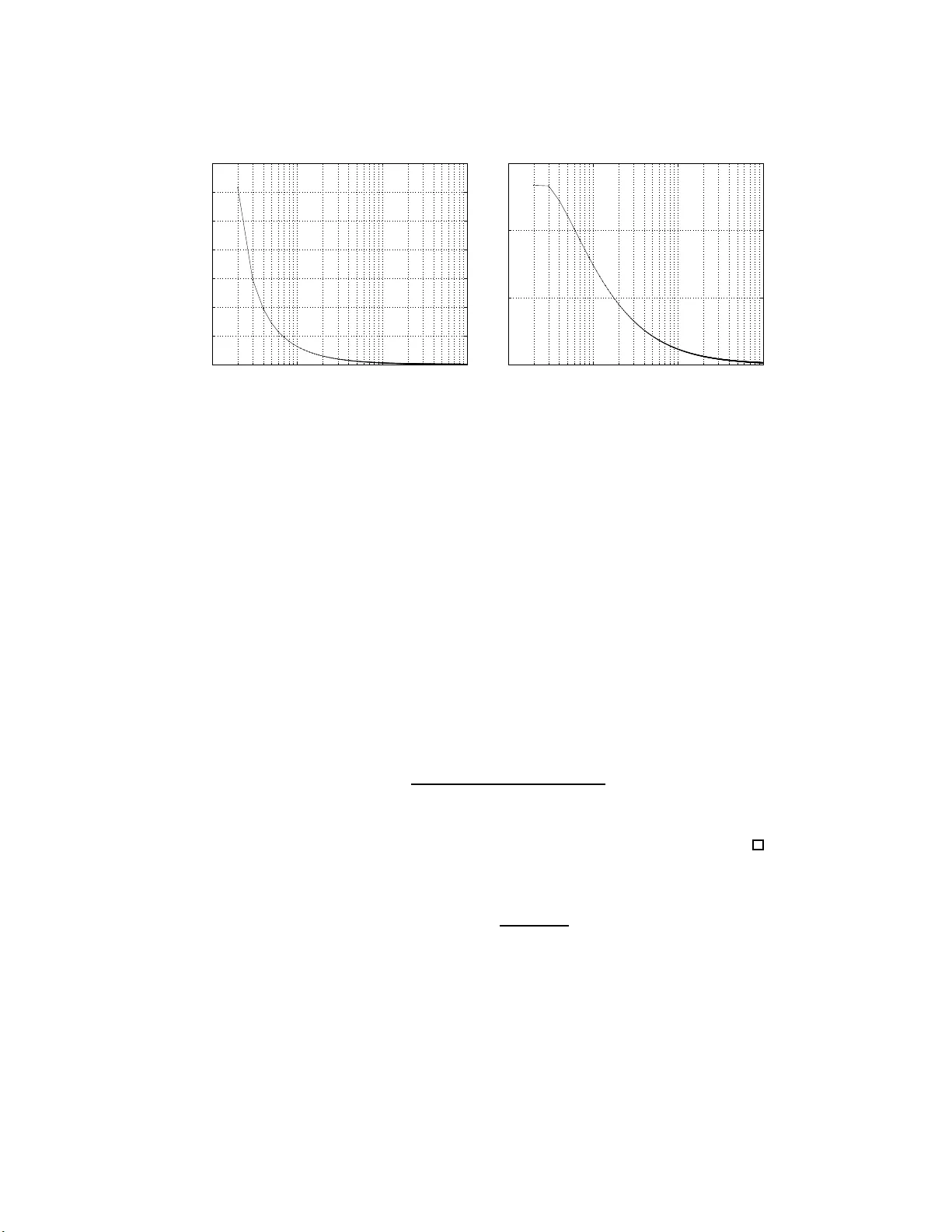
Estimatio n of a probabilit y in in v erse binomi al sampling under normali zed linear-linear and in v erse-li near loss Luis Mendo ∗ No v ember 4, 2018 Abstract Sequential es timation of the success probability p in in vers e binomial sam- pling is considered in this pap er. F or any estimator ˆ p , its qu alit y is measured by the risk associated with normalized loss functions of linear-linear or inv erse-linear form. These fun ctions are p ossibly asymmetric, with arbitrary slope parameters a and b for ˆ p < p and ˆ p > p resp ectively . Interest in these functions is motiv ated by their significance and potential uses, whic h are briefly discussed. Estimators are giv en for which th e risk has an asymp totic val ue as p → 0, and which gu ar- antee t hat, for any p ∈ (0 , 1), the risk is lo w er than its asympt otic v alue. This allo ws selecting th e requ ired number of successes, r , to meet a prescrib ed quality irrespective of the unk n ow n p . In addition, the prop osed estimators are shown to b e app ro ximately minimax when a/b do es not deviate too much from 1, and asymptotically minimax as r → ∞ when a = b . Keywor ds: Sequential estimation, Poin t estimator, I nv erse binomial sampling, Asymmetric loss function. 1 Motiv a tion and considered loss functions The estimation o f the succes s probability p of a se q uence of Ber noulli trials is a re- curring problem, arising in many br a nches of scienc e and e ngineering. The quality of a p oint estimator of p , denoted as ˆ p , ca n b e mea sured in terms of its risk , o r average loss asso cia ted with a c e r tain loss function L . Since a given error is mo s t meaningful when co mpared with the true v alue p , quality mea sures use d in practice ar e most of- ten no rmalized ones (Mendo, 2 012). This corresp onds to L b eing a function o f ˆ p/p , rather than of ˆ p . Common lo ss functions include normalized squa red er ror ( ˆ p/p − 1) 2 and nor malized absolute er ror | ˆ p/p − 1 | . Int erv al es timation can also b e analy z e d in terms o f a cer tain loss function (Berger, 1985, p. 64 ) such that the r esulting r isk is the confidence level asso ciated with a n estimation interv al. Fixed-sample approaches to this pr o blem suffer fr om the drawbac k that the re - quired size dep ends on the unknown parameter p , a nd th us cannot be determined in adv ance. Therefore a se quential pr o c e dur e is r equired, consis ting of a s topping rule , which yields a ra ndom sa mple size, and an estimator based on the observed sample. ∗ E.T.S. Ingenieros de T elecom unicaci´ on, Polytec hnic Universit y of Madrid, 28040 Madrid, Spain. E-mail: lmendo@grc.ssr.upm. es. 1 Sequential estimation in Bernoulli trials has b een studied by man y authors. Girshick et al (1946) intro duce a nd analy ze a general class of sequential pro cedures for the un bi- ased estimation of p . Using a similar appro ach, DeGro ot (19 59) gives criteria for the selectio n of appropr iate sampling plans for unbiased estimation o f functions of p , with estimator p erfor mance measur ed by v ariance . His work shows that the fixed- size and inv er se pr o cedures a re the only efficie nt sampling plans, i.e. the only o nes for which the Cramer -Rao bo und (or informa tion inequa lit y) ho lds with equal sign. Huber t and Pyke (20 00) fo cus o n the asymptotic b ehaviour as p → 0. In this set- ting, they consider estimation of powers of p , with a loss function given as squa red error lo s s multiplied by another p ow er of p . Bar an a nd Ma giera (2010) c arry out a similar asy mptotic analys is fo r a different los s function. Using a Bay esian approach, Cabilio and Robbins (197 5) and Cabilio (197 7) co ns ider s ymmetrized relative squared error loss (given as [( ˆ p − p ) / ( p (1 − p ))] 2 ) plus a fixed cost p er observ a tion, and find sequential pro c e dur es which minimize the Bayes ris k in the estimation o f p . A lvo (1977) studies sequential Bay es estimatio n fr om a mo r e g eneral p oint o f view, where the observ a tions a re no t necessa rily Bernoulli v aria bles, and consider ing s quared erro r loss. A par ticularly a ppea ling stopping rule, first discussed by Haldane (1945), is inverse binomial sampling (also known as negative bino mia l sa mpling). Given r ∈ N , this r ule consists o f taking as many observ atio ns as nec e s sary to obtain exactly r s uccesses. The random n umber of observ a tions, N , is a sufficient sta tistic for p (Lehmann and Casella, 1998, p. 101). The interest in this stopping r ule is motiv ated by the us eful prop er - ties of the obtained es timators. Namely , it has b een shown that for an estimator ˆ p = g ( N ) s uch that lim n →∞ ng ( n ) exists and is p o sitive, and for a genera l class of loss functions defined by certain regular ity conditio ns , the ris k has an asympto tic v a lue as p → 0 (Mendo, 2 012). Moreov er, estimato rs hav e b een found whos e risk for p arbitrar y is guaranteed not to exceed its as ymptotic v a lue, for the sp ecific cases of normalized mean s quared erro r (Mikulsk i and Smith, 1 976) (Sathe, 1 977), normalized mean abso lute err or (Mendo, 2 0 09) and confidence asso cia ted with a rela tive interv al (Mendo and Hernando, 2 006) (Mendo and Hernando, 2008) (Mendo and Hernando, 2010). This allows selecting an appropria te v a lue of r that meets a prescr ib e d ris k irresp ective of the unknown p . In all cases mentioned in the prec e ding paragr aph, the loss incurred by a nega tive error eq ua ls that of the corres po nding po sitive error . In practice, how ever, situatio n- sp ecific facto rs may render underestimatio n more or le s s co stly than ov erestimation (Christoffersen and Dieb old, 199 7) (Akdeniz, 2004). Cons ider for example p = 0 . 01 and tw o p oss ible v a lue s o f ˆ p , namely 0 . 019 a nd 0 . 001. The absolute error (normalized or other wise) is the same for b oth v alues of the estima to r, as is the squared er ror. Nevertheless, with the firs t estimate ˆ p is 1 . 9 times p , whereas with the second p is 10 times ˆ p . In many applica tions it may be advisable to assign a hig her loss to the second estimate. With abso lute err or, this co uld b e acco mplis hed by genera lizing the lo ss function to one with a different s lo p e on ea ch side. Denoting x = ˆ p/p , this generaliz ed loss is given by L ( x ) = ( a (1 − x ) if x ≤ 1 , b ( x − 1) if x > 1 , (1) with para meters a, b ≥ 0, ( a, b ) 6 = (0 , 0 ). This function, known as (nor malized) line ar-line ar loss, frequently aris es in a pplications; see for example Gra nger (19 69) and Christoffers e n and Dieb old (1997). Another pr op osed function (not consider ed in this pap er ) which gives different weigh ts to p ositive and negative errors is the line ar- exp onential lo s s, who se normalized version is L ( x ) = b [exp( a ( x − 1)) − a ( x − 1) − 1 ], 2 with para meters a 6 = 0, b > 0 (Akdeniz, 2004). The ratio a/b , in the linear -linear loss, or the para meter a , in the linear-exp one ntial, control the r elative imp ortanc e given to under e stimation and ov erestimation. No te that in bo th cases the los s due to underestimation is b ounded, unlike that of ov erestimation, which may b e arbitrar ily large. In certa in situatio ns it may b e meaningful to define loss a s prop or tional to ˆ p/p or p/ ˆ p , whic hever is la rgest. Thu s with the v alues in the previous example, the loss would b e pro po rtional to 1 . 9 and 10 r esp ectively . In the following, the func- tion s ( ˆ p, p ) = max { ˆ p/ p , p/ ˆ p } will b e r eferred to a s the symmet ric r atio o f ˆ p and p (the na me is motiv a ted by the fa ct that s ( ˆ p, p ) = s ( p, ˆ p )). The loss thus defined is inherently normalized, b ecause it o nly dep ends on ˆ p and p thro ugh x = ˆ p /p . Sub- tracting 1 in order to have a minimu m loss equal to 0, the loss function is expressed as L ( x ) = max { x, 1 /x } − 1. This function is unbounded for underestimation as well as for overestimation erro r s. In fact, its graph is s ymmetric ab out x = 1 if ˆ p , o r x , is rep- resented in log arithmic scale (this is obvious if L ( x ) is wr itten as ex p | log x | − 1). The risk corr esp onding to this loss is the mean s ymmetric ratio minus 1 , and r epresents a normalized measure of dissimilarity b etw ee n ˆ p a nd p , with smaller v alues corre sp ond- ing to better estima to rs. A g eneralizatio n is obtained, as b efore, by allowing different m ultiplicative para meters a, b ≥ 0, ( a, b ) 6 = (0 , 0) on each side o f the function: L ( x ) = ( a (1 /x − 1) if x ≤ 1 , b ( x − 1) if x > 1 . (2) This will b e referr ed to a s inverse-line ar los s. The loss function (2), in addition to providing a natural measure of estimation quality , na mely g eneralized mean symmetric ra tio, can be representative of incurred cost in sp ecific applications. In spite of this, it has not b een used pre v iously in the context o f e s timation pro blems, to the author ’s knowledge. As a n e x ample of appli- cation, cons ider the pro duction of a certain device which is sub ject to manufacturing defects, such as image s ensors for dig ital cameras. Several fa c tors in the pr o duction pro cess (s uch as the presence of dust pa rticles) may res ult in a sensor with sp ecific pixels systema tically showing inco r rect information. Since it would b e to o exp ensive to discard all senso rs that hav e so me defect, the commonly adopted s olution is as follows. Each pro duced sensor is tested, and if the num b er of defective pixels is no t to o large it is a ccepted. The lo catio n of s uch pixels is pe r manently recorde d in the ca mera, so that they can be co rrected as a pa rt of the pro cessing applied by the c a mera to generate the image. In high-quality ca mera mo dels, how e ver, it may be de s irable to use senso rs with an ex tr emely low num b er o f defects. A p ossible pr o cedure is to classify each pro duced sensor as “premium” o r “standard” , dep ending on whether the num ber o f pixel defects is extremely low o r mer ely a cceptable. Premium sensors ar e reserved for adv anced cameras, which inco rp orate high-quality lenses, whereas s tandard sensor s are mounted in cons umer-level ca mer as with average-quality lens e s. F or ease of expla nation, these t wo types of lenses will a lso b e refer red to as pr emium and standar d, resp ectively . The pro duction o f each type o f lens is a more deterministic pr o cess than that o f s ensors, and th us the num ber o f pro duced lenses of ea ch type is easily controlled. It will b e assumed that the manufacturer is prima rily interested in its premium line of ca meras. A num b er S o f sensors is to b e pro duced, and the a mount of premium lenses that will b e required needs to b e planned in a dv ance. T o this end, an estimate ˆ p is made of the pro po rtion p o f sensors that will turn out to b e of the premium type (this can b e done using in verse binomial sampling); and S ˆ p premium lenses ar e made 3 av a ilable. The actual pro po rtion of pr emium sensors, p , may b e lower than ˆ p , in which case some of the pr e mium lenses will b e left un used; o r it may b e greater, and then some of the premium sensors will not b e used. In either ca se, so me resour ces a re wasted. If the cost as so ciated with each unused part is a for a sensor and b for a le ns , the r isk computed from the loss function (2) is the av er age cost of wasted resour ces per assembled premium camer a unit. The r est of the pa p er analyzes inv erse binomial sampling under the loss functions (1) and (2). The first has a lr eady b een analyzed for the particular ca se a = b by Mendo (2009), a nd the genera lization to a 6 = b will b e seen to b e r ather stra ightf orward. The second function has not b een dea lt with b efore, to the autho r ’s knowledge, a nd its analysis tur ns out to b e more difficult. Although the main fo c us of the pap er is on the second, results for the fir st a r e also interesting by themselves. In each cas e, estimato rs are g iven in Section 2 s uch that the r isk for p ∈ (0 , 1) is guara nt eed to b e low er than its asymptotic v a lue. Section 3 discusses these results and makes a compar is on with the optimum p erformance tha t could b e achieved by using other estimators . It is shown that the prop osed es timators are approximately minimax if a/b is close to 1; and for a = b they a re asymptotica lly minimax as r → ∞ . Section 4 contains the pro o fs to all results. 2 Main results Consider a sequence o f Ber noulli trials with probability of succe s s p , and a r andom stopping time N given by inv erse binomial s ampling with r ∈ N . Let x ( i ) denote x ( x − 1) · · · ( x − i + 1), fo r x ∈ R , i ∈ N ; and x (0) = 1. The normalized lower incomplete gamma function is defined as γ ( t, u ) = 1 Γ( t ) Z u 0 s t − 1 exp( − s ) d s, (3) and satisfies the following well-kno wn r elationship (Abramowitz and Stegun, 1970, eq. (6.5.21)), which will b e use d throughout the pap er: γ ( t − 1 , u ) = γ ( t, u ) + u t − 1 exp( − u ) Γ( t ) . (4) The random v ariable N ha s a neg ative bino mial distribution, with pr obability function f r ( n ) = P [ N = n ] given b y f r ( n ) = ( n − 1) ( r − 1) p r (1 − p ) n − r / ( r − 1)! , n ≥ r . The corres p o nding distribution function will be denoted as F r ( n ). Similarly , the pr obability function of a binomial random v aria ble with par ameters n and p is denoted as b n,p ( i ) = n ( i ) p i (1 − p ) n − i /i !, 0 ≤ i ≤ r . F or a n a rbitrar y nonrandomized estimator ˆ p = g ( N ) and a loss function L ( ˆ p/ p ), the risk η ( p ) is η ( p ) = E[ L ( ˆ p/p )] = ∞ X n = r f r ( n ) L ( g ( n ) /p ) . (5) F or r ≥ 2 a nd a, b ≥ 0, the loss functions (1) and (2) satisfy the sufficient conditions of Mendo (20 12, theorem 1 ), and thus any estima tor ˆ p = g ( N ) with lim n →∞ ng ( n ) = Ω > 0 has an asy mptotic risk as p → 0, which can be computed as lim p → 0 η ( p ) = 1 ( r − 1)! Z ∞ 0 ν r − 1 exp( − ν ) L (Ω /ν ) d ν. (6) 4 In pa rticular, this ho lds for a ny estimator that can b e expressed as ˆ p = Ω N + d (7) with Ω > 0, d > − r . Consider a generic e stimator of the form (7). Denoting m = ⌊ Ω / p − d ⌋ , the risk asso ciated with the loss function (1 ) can b e written as η ( p ) = a ∞ X n = m +1  1 − Ω ( n + d ) p  f r ( n ) + b m X n = r  Ω ( n + d ) p − 1  f r ( n ) = − a ∞ X n = r  Ω ( n + d ) p − 1  f r ( n ) + ( a + b ) m X n = r  Ω ( n + d ) p − 1  f r ( n ) . (8) Particularizing to Ω = r − 1 a nd d = − 1, which yields the unifor mly minimum v aria nce un biased (UMVU) estimator (Mikulski and Smith, 197 6), a nd taking int o account the ident ities (Mendo, 200 9) f r − 1 ( n − 1) = ( r − 1) f r ( n ) ( n − 1) p for r ≥ 2 , n ≥ r, (9) F r − 1 ( n − 1) = F r ( n ) + (1 − p ) b n − 1 ,p ( r − 1) for r ≥ 2 , n ≥ r, (10) it is seen that, for r ≥ 2, the first summand in (8) beco mes 0, and η ( p ) = ( a + b ) m X n = r ( f r − 1 ( n − 1) − f r ( n )) = ( a + b )( F r − 1 ( m − 1 ) − F r ( m )) = ( a + b )(1 − p ) b m − 1 ,p ( r − 1) . (11) The case a = b = 1 is analyzed in Mendo (200 9). Comparing (1 1) with Mendo (2 009, eq. (12)), the expression of the risk for a, b ar bitrary is see n to b e a straig ht forward generaliza tion of that for a = b = 1. As a co ns equence, the following result ho lds. Theorem 1. Consider the loss function given by (1) with a , b ≥ 0 , ( a, b ) 6 = (0 , 0) . F or r ≥ 2 , the risk η ( p ) asso ciate d with the est imator ˆ p = ( r − 1 ) / ( N − 1) satisfies η ( p ) < lim p → 0 η ( p ) for any p ∈ (0 , 1) , (12) with lim p → 0 η ( p ) = ( a + b )( r − 1) r − 2 exp( − r + 1) ( r − 2)! . (13) In addition, as will b e s een in Section 3, under cer tain conditions this estimator approaches the asymptotica lly optimum estimator discussed in Mendo (20 12). F or the los s function (2), the risk a sso ciated with an estimator of the fo r m (7) can be decomp osed in a similar wa y as for (1). Namely , η ( p ) = η 1 ( p ) + η 2 ( p ) with η 1 ( p ) = a ∞ X n = m +1  ( n + d ) p Ω − 1  f r ( n ) , (14) η 2 ( p ) = b m X n = r  Ω ( n + d ) p − 1  f r ( n ) . (15) 5 Assuming d ≤ 0 in (14) a nd taking in to a ccount tha t, as p er (9), npf r ( n ) = r f r +1 ( n + 1), it follows that η 1 ( p ) ≤ a ∞ X n = m +1  np Ω − 1  f r ( n ) = ar Ω (1 − F r +1 ( m + 1 )) + a ( F r ( m ) − 1) , (16) with strict ineq ua lity if d < 0 . As for η 2 ( p ), assuming d ≥ − 1 , it stems fr o m (9) and (15) that η 2 ( p ) ≤ b m X n = r  Ω ( n − 1 ) p − 1  f r ( n ) = b Ω r − 1 F r − 1 ( m − 1) − bF r ( m ) , (17) with strict ineq uality if d > − 1 a nd m ≥ r . As a r esult of (16) and (17), for a ny d ∈ [ − 1 , 0] the r isk sa tisfies η ( p ) ≤ b Ω r − 1 F r − 1 ( m − 1 ) + ( a − b ) F r ( m ) − ar Ω F r +1 ( m + 1 ) + a  r Ω − 1  . (18) The right-hand side of (18 ) is greatly simplified if Ω is chosen as a ny v a lue ˜ Ω > 0 such that ar ˜ Ω − b ˜ Ω r − 1 = a − b , (19) for in that case, applying the identit y (10) , η ( p ) ≤ b ˜ Ω r − 1 ( F r − 1 ( m − 1) − F r ( m )) + ar ˜ Ω ( F r ( m ) − F r +1 ( m + 1 )) + a  r ˜ Ω − 1  = b ˜ Ω r − 1 (1 − p ) b m − 1 ,p ( r − 1) + ar ˜ Ω (1 − p ) b m,p ( r ) + a  r ˜ Ω − 1  . (20) The adv a ntage of this expressio n is that the terms (1 − p ) b m − 1 ,p ( r − 1) and (1 − p ) b m,p ( r ) lend themselves to ana ly sis mor e easily than the distr ibution functions in (18). The condition (19) on ˜ Ω has a single p ositive solutio n for a, b ≥ 0, ( a, b ) 6 = (0 , 0 ), namely ˜ Ω =        ( r − 1)  1 + a + b 2 b  q 1 + 4 ab ( r − 1)( a + b ) 2 − 1  for a, b > 0 , r − 1 for a = 0 , b > 0 , r for b = 0 , a > 0 . (21) It is e a sily seen that this r educes to p r ( r − 1) for a = b > 0. In addition, the following holds. Prop ositi on 1. The value of ˜ Ω given by (21) lies in the interval ( r − 1 , r ) for a, b > 0 . As a consequence o f Prop os ition 1, for any a, b ≥ 0 , ( a, b ) 6 = (0 , 0), the v alue ˜ Ω defined b y (21) satisfies ˜ Ω ∈ [ r − 1 , r ] . T aking into a ccount that ˆ p umvu = ( r − 1 ) / ( N − 1) is the UMVU estima to r a nd that ˆ p ml = r / N is the ma ximum likelihoo d (ML) estimator (Best, 19 74), the es timator ˆ p given by (7) with Ω ∈ [ r − 1 , r ] a nd d ∈ [ − 1 , 0] is seen to be a “reaso nable” one, in the s ense tha t it is “clos e ” to the UMVU and ML estimator s. As will b e seen in Section 3, in certain cas es the pr op osed e stimator is also close to the asymptotically optimum estimato r in the sense of Mendo (2 0 12). 6 10 0 10 1 10 2 10 3 10 −1 10 0 r ¯ η Figure 1: Ris k gua ranteed not to b e exceeded for inv erse-linea r loss (2) with a = b = 1 The preceding arguments justify that the estimator given by (7) with Ω ∈ [ r − 1 , r ] and d ∈ [ − 1 , 0] is w orth considering. In fact, fo r adequate choices of Ω and d , it satisfies the impo rtant prop er ty that the ris k is g uaranteed not to exceed its as ymptotic v a lue, as established by the next theo rem. Theorem 2. Consider the loss function given by (2) with a , b ≥ 0 , ( a, b ) 6 = (0 , 0) . F or r ≥ 2 , the estimator ˆ p = ˜ Ω / N with ˜ Ω given by (21) satisfies η ( p ) < lim p → 0 η ( p ) for any p ∈ (0 , 1) , (22) with lim p → 0 η ( p ) = a  r ˜ Ω − 1  +  ar ˜ Ω + b  ˜ Ω r − 1 exp( − ˜ Ω) ( r − 1)! . (23) 3 Discussion and additional prop erties 3.1 Significance of t he results It has b een shown in Sec tio n 2 that simila r results to those already known for mean absolute error, mea n squared error and confidence lev el also hold for gener alized mean a bsolute er ror (Theorem 1) and g eneralized mean symmetric ratio (Theorem 2). Spec ific a lly , it has b een prov ed that, for the pro p osed estimator s, sup p ∈ (0 , 1) η ( p ) = lim p → 0 η ( p ). In the following, ¯ η will denote the v alue of lim p → 0 η ( p ), or eq uiv alently sup p ∈ (0 , 1) η ( p ), fo r the estimators in Theorems 1 and 2. The imp ortance o f these results lies in the fact that no knowledge is required ab out p . Thus, given any desired v alue λ fo r the risk , an adequa te r ca n b e selected such that the r isk is guar a nteed no t to exceed λ , ir resp ective of p . Namely , it suffices to choose r as the minim um v alue for which ¯ η , computed from (13) or fro m (23), is les s than or equa l to λ . As an illustration, Figur e 1 depicts ¯ η a s a function o f r for the loss given by (2) with a = b = 1. It is seen, for ex a mple, that r = 75 suffices to guar antee a risk low er than 0 . 1 , tha t is, a mean symmetric ra tio low er than 1 . 1 . 7 3.2 Comparison with minimax estimators The presented re sults are v a lid for sp ecific estimators, given by (7) with certain fixed v alues for Ω a nd d . It is natura l to ask to what extent the results could b e improv ed by co ns idering other estimators , i.e. how muc h lower risks could b e guar anteed not to be exceeded (or equiv alently how muc h sup p ∈ (0 , 1) η ( p ) could b e reduced). By defini- tion, an estimato r tha t is optimum ac cording to this criterio n (i.e. which minimizes sup p ∈ (0 , 1) η ( p ) over a ll po ssible estimators), if it ex ists, is a minimax es timator. This question can b e addres sed on the basis o f the a nalysis in Mendo (2012). F or a, b > 0, bo th (1) a nd (2) satisfy the ass umptions of Mendo (201 2, theorem 3). This implies that there exis ts a v a lue of Ω, denoted as Ω ∗ , such that any estimato r ˆ p = g ( N ) with lim n →∞ ng ( n ) = Ω ∗ minimizes lim sup p → 0 η ( p ) over all estimator s , including rando mize d ones . Thus a n y such estimato r is asymptotica lly optimum, in the s e nse of achieving the minimum p oss ible lim sup p → 0 η ( p ). This minimum, which will b e denoted as η ∗ , restricts the v a lues λ that the risk can b e g uaranteed not to exceed for p arbitrar y . Namely , if an estimator guarantees that η ( p ) ≤ λ for a g iven λ , then necessarily λ ≥ η ∗ . As a consequenc e , the ris k ¯ η that is gua r anteed not to be exceeded b y the spe c ific estimator s considered in Section 2 is a t most ¯ η /η ∗ times larger than what could b e achieved by a minimax estimator. The v alue η ∗ is obtained as follows. Consider the lo ss function (1) firs t. F or Ω arbitrar y , (6) g ives lim p → 0 η ( p ) = ( a + b )Ω γ ( r − 1 , Ω) r − 1 − ( a + b ) γ ( r , Ω) + a  1 − Ω r − 1  . (2 4 ) Its deriv ative d dΩ lim p → 0 η ( p ) = ( a + b ) γ ( r − 1 , Ω) − a r − 1 (25) is seen to b e monotone increasing. Therefore the minimizing v alue Ω ∗ is unique, and is determined by the condition d(lim p → 0 η ( p )) / dΩ = 0 , that is, γ ( r − 1 , Ω ∗ ) = a a + b . (26) Setting Ω = Ω ∗ in (24), substituting (26) and making use o f (4), η ∗ = ( a + b )Ω ∗ r − 1 exp( − Ω ∗ ) ( r − 1)! . (27) The v a lue Ω ∗ can b e co mputed numerically fro m (26), a nd η ∗ is then obta ine d by means of (27). Regarding the loss function (2), for Ω arbitra ry (6 ) gives lim p → 0 η ( p ) = b Ω γ ( r − 1 , Ω) r − 1 + ( a − b ) γ ( r, Ω) − arγ ( r + 1 , Ω) Ω + a  r Ω − 1  . (28) Again, it is easily seen that d dΩ lim p → 0 η ( p ) = bγ ( r − 1 , Ω) r − 1 − ar (1 − γ ( r + 1 , Ω)) Ω 2 (29) is monotone incr easing, and thus there is a single minimizing v alue Ω ∗ , which satisfies Ω ∗ 2 r ( r − 1) = a (1 − γ ( r + 1 , Ω ∗ )) bγ ( r − 1 , Ω ∗ ) . (30) 8 0.2 0.3 0.4 0.5 0.6 0.7 0.80.9 1 2 3 4 5 1 1.2 1.4 1.6 1.8 2 2.2 a/b ¯ η/η ∗ r = 3 r = 10 r = 30 r = 100 (a) Li near-linear loss (1 ) 0.2 0.3 0.4 0.5 0.6 0.7 0.80.9 1 2 3 4 5 1 1.1 1.2 1.3 1.4 1.5 1.6 a/b ¯ η/η ∗ r = 3 r = 10 r = 30 r = 100 (b) In verse-linear l oss (2) Figure 2: Degradation factor ¯ η /η ∗ as a function of a/b a nd r F rom (4), (2 8) a nd (3 0), η ∗ =  a +  2Ω ∗ r − 1 − 1  b  γ ( r − 1 , Ω ∗ ) + ( b − a )Ω ∗ r − 1 exp( − Ω ∗ ) ( r − 1)! − a. (31) The expressions (30) and (31) allow n umerically computing η ∗ . Figure 2 s hows, for the loss functions and estimators co nsidered in Theorems 1 a nd 2, the degradatio n factor ¯ η /η ∗ as a function of a/b , with r as a para meter. As is seen, for a/b no t to o far from 1 the degrada tion factor is close to 1, that is, the considered estimators are nearly o ptim um. F urthermore, there is a v alue of a/ b for which ea ch estimator is precisely optimum, i.e. minimax, as established by the following. Prop ositi on 2. F or e ach of t he loss funct ions (1) and (2) , ther e exists a un ique value of the r atio a/b for which the estimator c onsider e d in The or em 1 or 2 r esp e ctively is minimax, that is, minimizes s up p ∈ (0 , 1) η ( p ) over al l (p ossibly r andomize d) estimators. F or the loss function (1) this value is given by a b = γ ( r − 1 , r − 1) 1 − γ ( r − 1 , r − 1) , (32) and for (2) it is determine d by t he c ondition γ ( r − 1 , ˜ Ω) 1 − γ ( r + 1 , ˜ Ω) = r ( ˜ Ω − r + 1) ˜ Ω( r − ˜ Ω) (33) with ˜ Ω as in (21) . 3.3 Minimaxit y for asymptotically large r in the case a = b The sp ecific v alues o f the ratio a/b determined by Prop ositio n 2 ca n b e shown to tend to 1 a s r → ∞ . Rela ted to this, the following establishes that for a = b the prop osed estimators are asymptotica lly minimax as r → ∞ . Prop ositi on 3. F or the loss functions (1) and (2) with a = b , e ach of the estima- tors c onsider e d in The or ems 1 and 2, resp e ctively, appr o aches a m inimax estimator asymptotic al ly as r → ∞ , in the sense t hat lim r →∞ ¯ η /η ∗ = 1 . 9 10 0 10 1 10 2 10 3 1 1.01 1.02 1.03 1.04 1.05 1.06 1.07 r ¯ η/η ∗ (a) Linear-linear loss (1) 10 0 10 1 10 2 10 3 1 1.0005 1.001 1.0015 r ¯ η/η ∗ (b) In verse-linear l oss (2) Figure 3: Degradation factor ¯ η / η ∗ for a = b as a function o f r As a consequence of this r esult, for a = b a nd large r the consider ed estimato rs are approximately optimum in the minimax sens e . This is illustra ted in Figure 3, whic h shows the degradatio n fa ctor ¯ η /η ∗ as a function of r . In fact, ¯ η /η ∗ is s e e n to b e very low even for small r , and in particular for the range of v alues of r that are commonly used in practice. Thus, for example, the mean absolute erro r (loss function (1) with a = b = 1 ) that is g uaranteed not to b e exceeded accor ding to Theor em 1 is within 1% of the minimax mean abso lute error for 7 ≤ r ≤ 1000. Similar ly , defining r isk as mea n symmetric ratio minus 1 (loss function (2) with a = b = 1), the risk that is gua ranteed not to b e exceeded as pe r T he o rem 2 is within 0 . 1% o f the minimax risk for the same range of v alues of r . 4 Pro ofs F or ρ ∈ N , ρ ≥ 2; µ ≥ ρ − 1; and t ∈ (0 , 1), let Y ρ ( µ, t ) b e defined as Y ρ ( µ, t ) = ( µ − 1 ) ( ρ − 1) t ρ − 1 (1 − t ) µ − ρ +1 ( ρ − 1 )! . (34) Pr o of of The or em 1. The result immediately stems from (1 1) and the a nalysis in Mendo (2009). Lemma 1. The fol lowing ine quality holds for r ≥ 2 , d ∈ [ − 1 , 0] , j ≥ 2 . r − 1 X i =1 ( i + d + 1) j > ( r + d ) j +1 j + 1 . (35) Pr o of. The sum in (35) can b e express e d as the are a cov ered by the r − 1 rectang le s of width 1 and height ( i + d + 1) j , i = 1 , . . . , r − 1 in Figure 4, or equiv alently as the shaded area comprised by r − 2 unit-width trap ezoids plus tw o half-width rectang le s . Since the curve ( x + d + 3 / 2 ) j touches the upp er vertices o f the trap ezoids and is 10 1 i r −1 ( x + d +3/2) j ( i + d +1) j · · · · · · x Figure 4: Illustration of (36) conv ex , the following ineq ua lity can b e wr itten: r − 1 X i =1 ( i + d + 1) j ≥ Z r − 3 / 2 1 / 2  x + d + 3 2  j d x + ( d + 2) j 2 + ( r + d ) j 2 = ( r + d ) j +1 j + 1 + ( r + d ) j 2 + ( d + 2) j  1 2 − d + 2 j + 1  . (36) F or j ≥ 3 the ter m 1 / 2 − ( d + 2) / ( j + 1) in (36) is nonnegative, which ensures that (35) holds. F or j = 2 , (36) reduces to r − 1 X i =1 ( i + d + 1) j ≥ ( r + d ) 3 3 + − 2 d 3 − 6 d 2 + 6 ( r − 2) d + 3 r 2 − 4 6 . (37) The second summand in (3 7) has a deriv ative with res pe c t to d equal to − d 2 − 2 d + r − 2, which is nonneg ative for d ∈ [ − 1 , 0 ], r ≥ 2. Thus this summand is low er b ounded by its v alue a t d = − 1 , i.e. (3 r 2 − 6 r + 4) / 6, which is p os itive. Ther e fore (35) als o holds for j = 2. Lemma 2. Given ρ , µ , Ω and δ such that ( i) ρ ∈ N , ρ ≥ 2 ; (ii) Ω ∈ [ ρ − 1 , ρ ] ; (iii) δ ∈ [ − 1 , 0] ; (iv) µ > ρ − 1 ; and (v) µ > Ω − δ − 1 , the fol lowing hold: (a) Y ρ ( µ, Ω / ( µ + δ + 1)) is a strictly incr e asing function of µ , with lim µ →∞ Y ρ ( µ, Ω / ( µ + δ + 1)) = Ω ρ − 1 exp( − Ω) / ( ρ − 1 )! . (38) (b) Y ρ +1 ( µ + 1 , Ω / ( µ + δ + 1)) is a str ictly incr e asing function of µ , with lim µ →∞ Y ρ +1 ( µ + 1 , Ω / ( µ + δ + 1)) = Ω ρ exp( − Ω) /ρ ! . (39) Pr o of. Accor ding to hypotheses (iv) and (v), it holds that µ > ρ − 1 and Ω / ( µ + δ + 1) < 1, and thus Y ρ ( µ, Ω / ( µ + δ + 1)) and Y ρ +1 ( µ + 1 , Ω / ( µ + δ + 1)) are w ell defined from (34). The pro of will b e c a rried out separately for par ts (a) a nd (b) of the Lemma. 11 (a) It is conv enien t to make the change of v aria ble t = Ω / ( µ + δ + 1), by which Y ρ ( µ, Ω / ( µ + δ + 1)) is expressed as Y ρ (Ω /t − δ − 1 , t ). It will b e shown that lim t → 0 Y ρ (Ω /t − δ − 1 , t ) = Ω ρ − 1 exp( − Ω) / ( ρ − 1 )! , (4 0 ) which is e q uiv alent to (38); a nd that Y ρ (Ω /t − δ − 1 , t ) is a str ictly decr easing function of t , which will imply that Y ρ ( µ, Ω / ( µ + δ + 1)) s trictly increases with µ . F r om (34), log Y ρ ( µ, t ) = ρ − 1 X i =1 log ( µ − i ) t Ω + ρ − 1 X i =1 log Ω i + ( µ − ρ + 1) log(1 − t ) , (41) and th us log Y ρ  Ω t − δ − 1 , t  = ρ − 1 X i =1 log  1 − ( i + δ + 1) t Ω  + ρ − 1 X i =1 log Ω i +  Ω t − ρ − δ  log(1 − t ) . (42) T aking into acco un t that ( ρ + δ ) t/ Ω = ( ρ + δ ) / ( µ + δ + 1) < 1 a s a result of (iv), and that t < 1, the T aylor expansio n log (1 − t ) = − P ∞ j =1 t j /j , | t | < 1 can b e used in (42) to yield log Y ρ  Ω t − δ − 1 , t  = − ∞ X j =0 c j t j , (43) c 0 = Ω + ρ − 1 X i =1 log i Ω , (44) c j = Ω j + 1 − ρ + δ j + 1 j Ω j ρ − 1 X i =1 ( i + δ + 1) j for j ≥ 1 . (45) The equalities (43) and (44) imply (40), and thus (38). T o prov e that Y ρ (Ω /t − δ − 1 , t ) stric tly decreases with t , it suffices to show that the co efficients c j satisfy c j ≥ 0, j ≥ 1, with strict inequality for some j . F or j ≥ 2, (45) and Lemma 1 yield j ( j + 1) c j > j Ω − ( j + 1)( ρ + δ ) + ( ρ + δ )  ρ + δ Ω  j = − j ( ρ + δ − Ω) + ( ρ + δ )  ρ + δ Ω  j − 1 ! . (46) T aking into a ccount tha t ρ + δ ≥ 0 by hypo thesis (iii), and using the inequa lit y  ρ + δ Ω  j =  1 + ρ + δ − Ω Ω  j ≥ 1 + j ( ρ + δ − Ω) Ω , (47) it follows from (46) that c j > ( ρ + δ − Ω) 2 ( j + 1 )Ω ≥ 0 . (48) 12 F or j = 1 , (45 ) gives c 1 = Ω 2 − 2 ρ Ω + ( ρ − 1)( ρ + 2) 2Ω + δ ( ρ − Ω − 1) Ω . (49) Consider the first summand in (49). The minim um o f its numerator with resp ect to Ω is attained at Ω = ρ and equals ρ − 2. T hus, acco rding to hypo thes is (i), this summand is nonnegative. By (ii) and (iii), the s econd summand is also nonnegative; and therefore c 1 ≥ 0. Cons equently Y ρ (Ω /t − δ − 1 , t ) strictly decrea ses with t , and th us Y ρ ( µ, Ω / ( µ + δ + 1)) str ictly increases with µ . (b) Making the same change of v ar iable as in part (a), a nd taking int o acc o unt (43)–(45), log Y ρ +1  µ + 1 , Ω µ + δ + 1  = log Y ρ +1  Ω t − δ, t  = − ∞ X j =0 c ′ j t j , (50) c ′ 0 = Ω + ρ X i =1 log i Ω , (51) c ′ j = Ω j + 1 − ρ + δ j + 1 j Ω j ρ − 1 X i =0 ( i + δ + 1) j ≥ c j for j ≥ 1 . (52) F rom (52) it follows tha t c ′ 1 ≥ 0 and c ′ j > 0 for j ≥ 2 . T o gether with (5 0) and (51 ), this establishes part (b) of the Lemma. Pr o of of The or em 2. As the ca se a = 0, b > 0 is already cov ered by Theorem 1 , it will be assumed that a > 0. This implies, according to Prop os ition 1, that ˜ Ω > r − 1 . The equa lity (23) is o btained subs tituting the loss function (2) into (6) with Ω = ˜ Ω, and making use of (4 ) and (19). The inequality (20) can b e expr essed a s η ( p ) ≤ b ˜ Ω Y r ( m, p ) r − 1 + arY r +1 ( m + 1 , p ) ˜ Ω + a  r ˜ Ω − 1  , (53) m = ⌊ ˜ Ω /p ⌋ . (54) F rom (54) it stems that m ≥ r − 1. Each v alue of m has an asso cia ted int erv al I m ⊆ (0 , 1) s uch tha t (54) holds if and only if p ∈ I m . Namely , I m = ( p l , p u ] with p l = ˜ Ω / ( m + 1), p u = ˜ Ω /m , ex c ept if m = r − 1, in which case ˜ Ω < r and th us p l < 1, p u > 1 ; or if m = r and ˜ Ω = r , which gives p l < 1 , p u = 1; in either ca se I m = ( p l , 1). According to (53), and taking in to ac count (19), to e s tablish (22) it suffices to show that, for p ∈ (0 , 1 ) a nd m given by (54), Y r ( m, p ) < ˜ Ω r − 1 exp( − ˜ Ω) / ( r − 1 )! , (55) Y r +1 ( m + 1 , p ) < ˜ Ω r exp( − ˜ Ω) /r ! . (56) If m = r − 1 the left-hand sides of (55) and (56) are zero, a nd the inequa lities a re clearly satisfied. Thus in the fo llowing it will b e as s umed tha t m ≥ r . As a step in the pro of of (55) a nd (56), it will b e shown that for p ∈ (0 , 1 ) a nd m ≥ r r elated by (54), o r equiv a lently for m ≥ r and p ∈ I m , the following inequalities 13 hold: Y r ( m, p ) ≤ ( Y r ( m, ( r − 1 ) /m ) if ( ˜ Ω − r + 1) m ≤ r − 1 , Y r ( m, ˜ Ω / ( m + 1)) if ( ˜ Ω − r + 1) m > r − 1 . (57) Y r +1 ( m + 1 , p ) ≤ ( Y r +1 ( m + 1 , r / ( m + 1 )) if ( r − ˜ Ω) m ≤ ˜ Ω , Y r +1 ( m + 1 , ˜ Ω /m ) if ( r − ˜ Ω) m > ˜ Ω . (58) F or m ≥ r , it follows from (34) tha t Y r ( m, p ) considered as a function of p ∈ (0 , 1) is maximum at p max = ( r − 1 ) /m < 1, monotone increas ing for p < p max , and monotone decreasing for p > p max . As ˜ Ω > r − 1, it is seen that p max < p u ≤ 1, and that p max < p l if and only if ( ˜ Ω − r + 1) m > r − 1. This implies that Y r ( m, p ) is bo unded as given by (57). Regarding (58), the maximum of Y r +1 ( m + 1 , p ) with r esp ect to p ∈ (0 , 1) is a ttained at p ′ max = r / ( m + 1) < 1. As m ≥ r , it stems that p l ≤ p ′ max < 1, and that p u < p ′ max if and only if ( r − ˜ Ω) m > ˜ Ω. This establishes (58). The pr o of o f (55) will be ba s ed on (57). Since ˜ Ω > r − 1, the following definition can be made: µ 1 = ( r − 1) / ( ˜ Ω − r + 1). The fact that ˜ Ω ≤ r implies that µ 1 ≥ r − 1. The upp er condition in (57) is equiv alent to m ≤ µ 1 , whe r eas the low er corr esp onds to m > µ 1 . As m canno t b e smaller than r , the c ondition m ≤ µ 1 can only b e met for some m if µ 1 ≥ r , i.e. if ˜ Ω ≤ r − 1 /r . On the other hand, the c ondition m > µ 1 can alwa ys be satis fied by taking m sufficiently large. Th us, (55) will b e established in tw o steps. First, it will b e shown that Y r ( m, ˜ Ω / ( m + 1)) monoto nically incr eases with m > µ 1 and tends to ˜ Ω r − 1 exp( − ˜ Ω) / ( r − 1)! as m → ∞ . This will prov e that (55) holds for all m > µ 1 . Second, it will b e shown, for µ 1 ≥ r , that Y r ( m, ( r − 1) /m ) monotonically increases with m ≥ r and is smaller than ˜ Ω r − 1 exp( − ˜ Ω) / ( r − 1)! for m = µ 1 . This will esta blis h (5 5) for all m such that r ≤ m ≤ µ 1 . Regarding the first ca se, m > µ 1 , consider Lemma 2(a) with v alues r , m , ˜ Ω, 0 resp ectively for ρ , µ , Ω, δ . These v a lues satisfy the hypotheses of the Lemma (it is obvious that (i)–(iii) ho ld; (iv) and (v) ar e satis fie d a s well b ecause m > µ 1 ≥ r − 1 ≥ ˜ Ω − 1). Accor ding to this, Y r ( m, ˜ Ω / ( m + 1)) mono tonically increase s with m and tends to ˜ Ω r − 1 exp( − ˜ Ω) / ( r − 1 )! a s m → ∞ . Therefor e (55 ) holds for m > µ 1 . F or the cas e r ≤ m ≤ µ 1 , µ 1 ≥ r , using Lemma 2 (a) (with v alues r , m , r − 1 , − 1 resp ectively for ρ , µ , Ω, δ ; (iv) and (v) hold be cause m ≥ r ) it is seen that Y r ( m, ( r − 1) /m ) increases with m . The definition of µ 1 implies that ( r − 1) /µ 1 = ˜ Ω / ( µ 1 + 1), and thus Y r ( µ 1 , ( r − 1) /µ 1 ) = Y r ( µ 1 , ˜ Ω / ( µ 1 + 1)) . (59) Applying Lemma 2(a) ag ain (with v a lues r , µ 1 , ˜ Ω, 0; no te that (v) is satisfied b ecaus e µ 1 ≥ r ≥ ˜ Ω > ˜ Ω − 1) to the right-hand side of this equality s hows that (59) is s maller than ˜ Ω r − 1 exp( − ˜ Ω) / ( r − 1)!. Therefo re (55) ho lds for r ≤ m ≤ µ 1 . As for (56), it is se e n that the low er condition in (58) is not met fo r any m if ˜ Ω = r , whereas if ˜ Ω < r there exist v alues of m which satisfy each o f the conditions. These t wo cases will b e tr eated separately . In the case ˜ Ω < r , the pro o f pro ceeds along the same lines a s that of (55). Let µ 2 = ˜ Ω / ( r − ˜ Ω). The fact that ˜ Ω > r − 1 implies that µ 2 > r − 1. In a ddition, since m ≥ r , the upp er co ndition in (58) can only b e met if µ 2 ≥ r . Thus it suffices to show first that Y r +1 ( m + 1 , ˜ Ω /m ) mo notonically inc r eases with m > µ 2 and tends to ˜ Ω r exp( − ˜ Ω) /r ! as m → ∞ ; and seco nd that, if µ 2 ≥ r , Y r +1 ( m + 1 , r / ( m + 1)) monotonically incr eases with m ≥ r and is smaller than ˜ Ω r exp( − ˜ Ω) /r ! for m = µ 2 . The first pa r t directly s tems fro m Lemma 2(b) (with v a lues r , m , ˜ Ω, − 1 ). As for the 14 second, the incr easing character of Y r +1 ( m + 1 , r / ( m + 1)) with m is also established by Lemma 2(b) (with v a lues r , m , r , 0 ). The definition of µ 2 implies that r / ( µ 2 + 1) = ˜ Ω /µ 2 , from which Y r +1 ( µ 2 + 1 , r / ( µ 2 + 1)) = Y r +1 ( µ 2 + 1 , ˜ Ω /µ 2 ) , (60) and a pplying Lemma 2(b) (with v alues r , µ 2 , ˜ Ω, − 1; (iv) a nd (v) hold b eca us e µ 2 = ˜ Ω / ( r − ˜ Ω) > ˜ Ω > r − 1) to the right-hand side of (60) establishes that it is smaller than ˜ Ω r exp( − ˜ Ω) /r !. In the case ˜ Ω = r , the expr ession (58 ) reduces to its upp er part, and (56) follows from Lemma 2(b) (with v alues r , m , r , 0 ). This completes the pro of. Pr o of of Pr op osition 2. F or L as in (1), equating d(lim p → 0 η ( p )) / dΩ given by (25) to 0, solving for a/b and par ticularizing to Ω = r − 1 y ields (32). As for L given by (2), from (19) it is seen that a b = ( ˜ Ω − r + 1) ˜ Ω ( r − 1)( r − ˜ Ω) . (61) Setting Ω ∗ = ˜ Ω in (30) and co mbining with (61) yields (33). Lemma 3. F or any k ∈ N , the factorial k ! satisfies the fol lowing: k ! > √ 2 π k k +1 / 2 exp( − k ) , (62) lim k →∞ k ! exp( k ) k k +1 / 2 = √ 2 π . (63) Pr o of. These expressio ns follow from Abramowitz and Stegun (1970, eq. (6.1.38)). Lemma 4. F or any se quenc e of numb ers δ k such that 0 ≤ δ k ≤ 1 , lim k →∞ γ ( k , k + δ k ) = 1 / 2 . Pr o of. Accor ding to Adell a nd Jo dr´ a (20 05, le mma 1), lim k →∞ γ ( k , k ) = 1 / 2 . F rom (4), γ ( k , k + 1) − γ ( k + 1 , k + 1 ) = ( k + 1) k exp( − k − 1 ) / k ! . (64) As a result of Lemma 3, the right-hand s ide of (64) tends to 0 as k → ∞ , and therefore lim k →∞ γ ( k , k + 1) = lim k →∞ γ ( k , k ) = 1 / 2. The fact that γ ( t, u ) is monotone increasing in u implies that γ ( k , k ) ≤ γ ( k , k + δ k ) ≤ γ ( k , k + 1), and the desired res ult follows. Lemma 5. F or r ≥ 2 and a = b , the solution Ω ∗ to (2 6) lies in ( r − 4 / 3 , r − 2 + log 2) , and lim r →∞ (Ω ∗ − r ) = − 4 / 3 . Pr o of. The res ult follows fr om Alm (200 3). Lemma 6. F or r ≥ 2 and a = b , the solution Ω ∗ to (30) lies in ( r − 1 , r ) . Pr o of. Using (4) the condition (30) can be written, for a = b , a s  Ω ∗ 2 r ( r − 1) + 1  γ ( r, Ω ∗ ) = Ω ∗ r exp( − Ω ∗ ) r !  1 − Ω ∗ r − 1  + 1 . (65) Let v 1 (Ω ∗ ) and v 2 (Ω ∗ ) resp ectively denote the left-hand a nd r ight-hand sides of (6 5), considered as functions of Ω ∗ . It is ea sily seen that v 1 is monotone incr easing, whe r eas 15 v 2 is monotone decr easing o n the interv al ( r − 1 , r ). F rom Lemma 5 and the mono- tonicity of γ ( t, u ) with resp ect to u it follows that γ ( r, r − 1) < 1 / 2, which implies that v 1 ( r − 1) < 1. O n the other hand, v 2 ( r − 1) = 1. Therefore the so lution to (65), or equiv a lent ly to (3 0), satisfies Ω ∗ > r − 1 . By analogo us arguments it is se e n that v 1 ( r ) > 1 and v 2 ( r ) < 1. Ther efore the solution satisfies Ω ∗ < r . Lemma 7 . F or any δ 1 , δ 2 ∈ R , t he se quenc e of functions h k ( δ ) = exp( δ )(1 + δ / ( k − 1)) − k +1 , k ∈ N , k ≥ 2 , δ ∈ [ δ 1 , δ 2 ] c onver ges un iformly to 1 as k → ∞ . Pr o of. Let k 0 = max {− δ 1 , 0 } + 2. As 1 + δ / ( k − 1) > 0 for δ ≥ δ 1 , k ≥ k 0 , it is p ossible to take loga rithms in the definition o f h k ( δ ) for k ≥ k 0 , whic h gives log h k ( δ ) = δ − ( k − 1) log(1 + δ / ( k − 1)). Replacing k b y a co nt inuous v ariable x > 1 and using the inequality log (1 + t ) > t/ (1 + t ), it is s een that ∂ ∂ x  δ − ( x − 1) log  1 + δ x − 1  = − log  1 + δ x − 1  + δ x + δ − 1 < 0 . (66) This implies tha t h k +1 ( δ ) < h k ( δ ) for k ≥ k 0 . In addition, h k ( δ ), δ ∈ [ δ 1 , δ 2 ] is a contin uous function and conv erges p oint wise to 1 a s k → ∞ . Thus Dini’s theorem (Apos tol, 19 74, p. 2 4 8) can b e a pplied, w hich ensur e s that the co nv er gence is unifor m. Pr o of of Pr op osition 3. F or L as in (1), particular iz ing (24) to a = b , Ω = r − 1 and using (4), ¯ η a = 2 ( γ ( r − 1 , r − 1) − γ ( r, r − 1)) = 2( r − 1) r − 2 exp( − r + 1) ( r − 2)! . (67) In the following, the v alue Ω ∗ determined b y (26) for a given r w ill b e denoted as Ω ∗ r . Particularizing (27) to a = b , η ∗ a = 2Ω ∗ r r − 1 exp( − Ω ∗ r ) ( r − 1)! . (68) F rom (67) and (68), with h k ( δ ) as defined in Lemma 7, it follows that ¯ η η ∗ =  r − 1 Ω ∗ r  r − 1 exp(Ω ∗ r − r + 1) = h r ( δ ∗ r ) (69) with δ ∗ r = Ω ∗ r − r + 1. Lemma 5 establishes tha t δ ∗ r ∈ [ − 1 / 3 , − 1 + lo g 2] and lim r →∞ δ ∗ r = − 1 / 3. On the other hand, by Lemma 7, h k → 1 uniformly on [ − 1 / 3 , − 1 + log 2 ] a s k → ∞ . Therefore, accor ding to Ap ostol (1974, theorem 9 .1 6), lim k,l →∞ h k ( δ ∗ l ) ex ists and equa ls 1. Thus, in particular , lim r →∞ h r ( δ ∗ r ) = 1, which combined with (69) establishes that lim r →∞ ¯ η /η ∗ = 1 . F or L as in (2), and with Ω ∗ given by (30), let Ω ∗ r and δ ∗ r be defined as b efor e. In addition, let ˜ Ω r denote the v alue of ˜ Ω corres po nding to a g iven r , and ˜ δ r = ˜ Ω r − r + 1. Particularizing (28) to a = b , Ω = ˜ Ω r and using (4) gives ¯ η a = r ˜ Ω r ( γ ( r − 1 , ˜ Ω r ) − γ ( r + 1 , ˜ Ω r )) + ˜ Ω r r − 1 − r ˜ Ω r ! γ ( r − 1 , ˜ Ω r ) + r ˜ Ω r − 1 = ˜ Ω r − 1 r exp( − ˜ Ω r ) ( r − 1)!  1 + r ˜ Ω r  + ˜ Ω r r − 1 − r ˜ Ω r ! γ ( r − 1 , ˜ Ω r ) + r ˜ Ω r − 1 . (70) 16 Thu s ¯ η can b e wr itten as a ( ˜ θ 0 + ˜ θ 1 + ˜ θ 2 ) with ˜ θ 0 = ( r − 1 + ˜ δ r ) r − 2 exp( − r + 1 − ˜ δ r ) ( r − 2)! 2 + 1 + ˜ δ r r − 1 ! , (71) ˜ θ 1 = ˜ δ 2 r r − 1 + 2 ˜ δ r − 1 r − 1 + ˜ δ r γ ( r − 1 , r − 1 + ˜ δ r ) , (72) ˜ θ 2 = 1 − ˜ δ r r − 1 + ˜ δ r . (73) The quotient ˜ θ 2 / ˜ θ 0 is computed as ˜ θ 2 ˜ θ 0 = (1 − ˜ δ r ) exp( ˜ δ r )  1 + ˜ δ r r − 1  r − 1  2 + 1+ ˜ δ r r − 1  · ( r − 1)! exp ( r − 1) ( r − 1) r − 1 / 2 · 1 √ r − 1 . (74) Prop ositio n 1 implies that ˜ δ r ∈ (0 , 1). T aking int o account that r ≥ 2, it is see n that the first factor in (7 4) lies in a b ounded interv al fo r all r , where as, by the equality in Lemma 3, the se cond factor tends to √ 2 π as r → ∞ . As a result, lim r →∞ ˜ θ 2 / ˜ θ 0 = 0. Similarly , ˜ θ 1 / ˜ θ 0 is express ed as ˜ θ 1 ˜ θ 0 =  ˜ δ 2 r r − 1 + 2 ˜ δ r − 1  exp( ˜ δ r )  1 + ˜ δ r r − 1  r − 1  2 + 1+ ˜ δ r r − 1  · ( r − 1)! exp ( r − 1) ( r − 1) r − 1 / 2 · γ ( r − 1 , r − 1 + ˜ δ r ) · 1 √ r − 1 . (75) As b efor e, the first factor in the right-hand side of (75) is b ounded, a nd the s econd tends to √ 2 π . The third factor tends to 1 / 2 by Lemma 4. Thus lim r →∞ ˜ θ 1 / ˜ θ 0 = 0. The quotient η ∗ /a is given as in (70) with ˜ Ω r replaced by Ω ∗ r ; and η ∗ = a ( θ ∗ 0 + θ ∗ 1 + θ ∗ 2 ), where θ ∗ 0 , θ ∗ 1 and θ ∗ 2 are obta ine d from (7 1)–(73) with ˜ δ r replaced by δ ∗ r . Lemma 6 implies that δ ∗ r ∈ (0 , 1), and ar guments analogo us to those in the pr e c eding parag raph show that θ ∗ 1 /θ ∗ 0 and θ ∗ 2 /θ ∗ 0 tend to 0 as r → ∞ . As a result, lim r →∞ ¯ η /η ∗ can b e computed as lim r →∞ ¯ η η ∗ = lim r →∞ ˜ θ 0 θ ∗ 0 = lim r →∞  1 + ˜ δ r r − 1  r − 2 exp( − ˜ δ r )  1 + δ ∗ r r − 1  r − 2 exp( − δ ∗ r ) · 2 + 1+ ˜ δ r r − 1 2 + 1+ δ ∗ r r − 1 . (76) Since ˜ δ r , δ ∗ r ∈ (0 , 1) for all r , it is clear that the second factor in the rightmost part of (76) tends to 1 as r → ∞ . By Le mma 7, (1 + δ / ( r − 1)) r − 1 exp( − δ ) → 1 uniformly for δ ∈ (0 , 1 ). This implies that the numerator and deno minator of the first facto r in (76) tend to 1 as r → ∞ (note that ˜ δ r and δ ∗ r are not r equired to conv erge). Co nsequently lim r →∞ ¯ η /η ∗ = 1. References Abramowitz M, Steg un IA (eds) (1970) Handb o ok of Mathematical F unctions, nin th edn. Dov e r Adell JA, Jo dr´ a P (2005) The media n o f the Poisson distribution. Me trik a 61:33 7–346 17 Akdeniz F (200 4) New biased estimator s under the linex los s function. Statistical Papers 45:17 5–19 0 Alm SE (2003) Monotonicity of the difference b etw een median and mean of gamma distributions and of a rela ted Rama nujan s equence. Bernoulli 9(2):35 1–37 1 Alvo M (1977) Bayesian sequential estimation. Annals of Statistics 5(5 ):955–9 68 Apo s tol TM (1974 ) Mathematical Analys is , 2nd edn. Addison-W esley Baran J , Ma giera R (2010) Optimal sequential estimation pro c e dur es o f a function of a probability of success under LINE X loss. Statistical Pape r s 5 1(3):511– 529 Berger JO (1985) Sta tis tica l Decision Theory a nd Bayesian Analysis, 2nd e dn. Springer-V erlag Best DJ (1974 ) The v a riance of the inv erse bino mial estimator. B iometrik a 61(2):3 85– 386 Cabilio P (1 9 77) Sequential estimation in B ernoulli trials . Annals of Sta tistics 5(2):342 – 356 Cabilio P , Robbins H (1975 ) Sequent ial estimation of p with squar ed relative err or loss. Pro ceeding s of the National Academy of Sciences of the United States of America 72(1):191 –193 Christoffersen P F, Dieb old FX (19 97) Optimal prediction under asymmetric loss. Econometric Theory 13:80 8–81 7 DeGro ot MH (1959) Unbiased sequential estimatio n for bino mial p opulatio ns. Annals of Mathematical Statistics 30 (1):80–10 1 Girshick MA, Mo steller F, Sav age LJ (194 6) Unbiased estimates for certain bino mial sampling pro blems with applications. Anna ls o f Mathematical Statistics 17(1):13 –23 Granger CWJ (19 69) Prediction with a ge ne r alized cos t of error function. Op eratio nal Research Quar ter ly 2 0 (2):199– 207 Haldane JBS (194 5 ) O n a method of estimating frequencies. Biometrik a 3 3(3):222– 225 Huber t SL, P y ke R (2000 ) Sequential estimation of functions of p for Ber noulli tr i- als. In: Game Theor y , Optimal Stopping, Pro ba bility and Statistics, Institute of Mathematical Statistics, pp 263 –294 Lehmann EL, Casella G (19 98) Theo ry of Poin t Estimation, 2nd edn. Springer Mendo L (200 9) Estimation of a proba bility with guara nteed normalized mean absolute error . IEEE Communications Letter s 1 3(11):81 7 –819 Mendo L (20 12) Asy mptotically optimum estimation of a probability in inverse bino- mial sampling. Journa l of Statistical Pla nning and Inference 142 (10):286 2–287 0. Mendo L, Hernando JM (20 0 6) A simple s equential stopping rule for Monte Carlo simulation. IEEE T ransactions on Communications 54 (2):231– 2 41 Mendo L, Hernando JM (20 08) Improved sequential stopping rule for Monte Carlo simulation. IEEE T ransactions on Communications 56 (11):176 1 –176 4 18 Mendo L, Hernando JM (2010) Estimatio n of a probability with optimum g uaranteed confidence in inv e r se bino mial sampling. Bernoulli 16(2 ):493–5 13 Mikulski P W, Smith PJ (19 76) A v ariance bound for unbiased estimation in inv erse sampling. Biometrik a 63(1 ):2 16–21 7 Sathe YS (19 77) Sharp er v a riance b ounds for unbiased estimatio n in inv erse sampling. Biometrik a 64(2):42 5–42 6 19