Parameterization of Sequence of MFCCs for DNN-based voice disorder detection
In this article a DNN-based system for detection of three common voice disorders (vocal nodules, polyps and cysts; laryngeal neoplasm; unilateral vocal paralysis) is presented. The input to the algorithm is (at least 3-second long) audio recording of sustained vowel sound /a:/. The algorithm was developed as part of the “2018 FEMH Voice Data Challenge” organized by Far Eastern Memorial Hospital and obtained score value (defined in the challenge specification) of 77.44. This was the second best result before final submission. Final challenge results are not yet known during writing of this document. The document also reports changes that were made for the final submission which improved the score value in cross-validation by 0.6% points.
💡 Research Summary
**
The paper presents a deep‑neural‑network (DNN) based system for automatically detecting three common voice disorders—vocal nodules/polyps/cysts, laryngeal neoplasm, and unilateral vocal paralysis—from recordings of a sustained vowel /a:/. The work was developed for the 2018 FEMH Voice Data Challenge, where it achieved the second‑best overall score (77.44) on the hidden test set.
Data and Pre‑processing
The challenge provided 200 training recordings (50 normal, 150 pathological) sampled at 44.1 kHz. Each file may contain several attempts at the vowel; a custom voice activity detection (VAD) pipeline extracts individual vowel segments. The VAD uses a 6th‑order low‑pass Butterworth filter (≤ 1000 Hz), Hilbert envelope extraction, moving‑average smoothing (1100‑sample window), and a threshold based on the 2nd and 95th percentiles of the envelope level plus 3 dB. Segments shorter than 500 ms are discarded, nearby segments (< 200 ms apart) are merged, and a 150 ms pre‑ and 250 ms post‑margin is added. This yields 213 vowel excerpts from the training set.
Data Augmentation
For each excerpt three augmented versions are generated by random volume scaling (0.4–1.2), pitch shifting (Gaussian, σ = 0.5 semitones), and time‑stretching (0.85–1.5×). Together with the original, the training pool expands to 852 samples, helping to mitigate the class imbalance (normal : pathological = 1 : 3).
Feature Extraction
Three complementary MFCC‑based representations are computed:
-
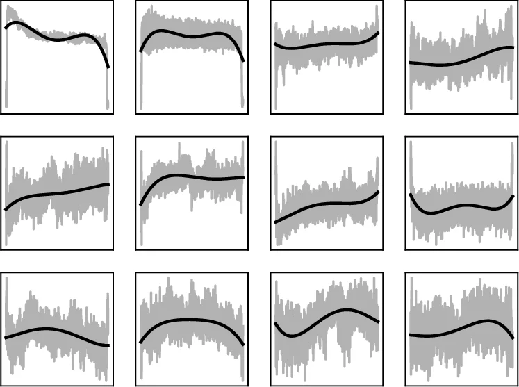
MFCC Polynomials – 13 MFCC coefficients (13 mel filters, 26‑filter bank, 13‑dimensional output) are extracted with a 8 ms window, 11 ms hop, 512‑point FFT, and a pre‑emphasis of 0.97. For each coefficient a 4th‑order polynomial is fitted over the entire frame sequence, yielding 5 coefficients per MFCC (65 features).
-
MFCC Splines – The first 50 frames (~0.5 s) are modeled with a spline that has knots at frames 0, 10, 20, 30, 40, 50. The spline values at these six positions are taken as features, giving 6 × 13 = 78 dimensions. If a sample is shorter than 50 frames, the last frame is repeated.
-
MFCC‑FFT – For the first 150 frames (≈2 s) the magnitude spectrum of each MFCC trajectory is computed via FFT; the first six magnitude bins are retained, resulting in another 78 features. This captures the rate of change rather than the exact shape.
In addition, two conventional voice‑quality descriptors are concatenated:
- Jitter – five jitter‑related measures (absolute jitter, RAP, PPQ5, DDP), fundamental frequency (F0), and harmonic‑to‑noise ratio (HNR) → 7 features.
- Cyclestarts – Turbulent Noise Index and Normalized First Harmonic Energy → 2 features.
Depending on the model version, the final feature vector contains 74 (polynomials + jitter + cyclestarts), 152 (polynomials + splines + jitter + cyclestarts), or 221 (polynomials + splines + FFT) dimensions.
Neural Network Architecture
A fully‑connected DNN with two hidden layers (128 neurons each) is employed. Hidden layers use Exponential Linear Units (ELU) and batch normalization. Dropout is applied before each layer (55–60 % before the first hidden layer, 25 % before the second, and 10 % before the output). The output layer has four neurons with softmax activation, representing the four classes (normal, phonotrauma, neoplasm, vocal palsy).
Training uses categorical cross‑entropy loss optimized with Adam (initial LR = 0.001, multiplied by 0.985 after each epoch). Each fold is trained for 100 epochs with batch size 32. To compensate for the smaller number of normal samples, normal recordings are presented twice per epoch from mid‑October onward.
Cross‑validation and Ensemble
A 5‑fold cross‑validation scheme is repeated 20 times with different random seeds, yielding 100 independently trained models. For each fold‑seed the best epoch (based on validation loss) is selected. At inference time, the probabilities from all 100 models are averaged, forming a strong ensemble.
Scoring Metric
The challenge score is a weighted average of Sensitivity (0.4), Specificity (0.2), and Unweighted Average Recall (UAR, 0.4). Sensitivity and Specificity are computed for a binary normal vs any‑pathology decision; UAR evaluates the three pathological categories separately.
Results
| Model | Features | Sensitivity | Specificity | UAR | Score (CV) |
|---|---|---|---|---|---|
| August | Polynomials + Jitter + Cyclestarts (74) | 89.9 % | 80.5 % | 67.47 % | 79.03 |
| Mid‑Oct | Polynomials + Splines + Jitter + Cyclestarts (152) | 90.7 % | 86.9 % | 60.63 % | 77.91 |
| Final | Polynomials + Splines + FFT (221) | 92.0 % | 85.9 % | 62.0 % | 78.52 |
On the hidden test set (reported by the organizers) the August model scored 76.33, while both the Mid‑Oct and Final models achieved the published 77.44, placing the authors’ submission second overall. The Final model shows the highest sensitivity (92 %) and a respectable specificity (85.9 %), indicating strong ability to detect pathological voices while maintaining a moderate false‑positive rate.
Discussion and Contributions
The core novelty lies in explicitly modeling the temporal evolution of each MFCC coefficient rather than treating each frame independently. By fitting low‑order polynomials, splines, and FFT‑based spectra, the authors compress the entire time series into a small set of interpretable parameters that capture onset dynamics, overall trend, and frequency of change. This approach yields a compact yet informative representation, enabling a relatively shallow DNN to achieve competitive performance without resorting to large convolutional or recurrent architectures.
Combining these MFCC‑derived descriptors with jitter and cyclestarts enriches the feature space with complementary information about voice stability and the acoustic characteristics of vowel onset/offset. The extensive data augmentation and ensemble strategy further improve robustness to variability in recording conditions and speaker differences.
Limitations include the fixed polynomial degree (4) and spline knot placement, which may not adapt optimally to all pathological patterns. The low‑pass filtering at 1 kHz removes high‑frequency content that could be diagnostic for certain lesions. Moreover, hyper‑parameter tuning was performed manually; automated search could potentially yield better network configurations.
Future Directions
Potential extensions involve adaptive polynomial degrees, data‑driven spline knot selection, or replacing the handcrafted temporal parameterization with sequence models such as LSTMs or Transformers that can learn temporal dependencies directly. Integrating additional modalities (e.g., laryngeal imaging) or employing multi‑task learning to jointly predict pathology type and severity could further enhance clinical utility. Finally, calibrating the decision threshold to balance sensitivity and specificity according to specific screening scenarios would be essential for real‑world deployment.
Comments & Academic Discussion
Loading comments...
Leave a Comment