Achieving Human Parity in Conversational Speech Recognition

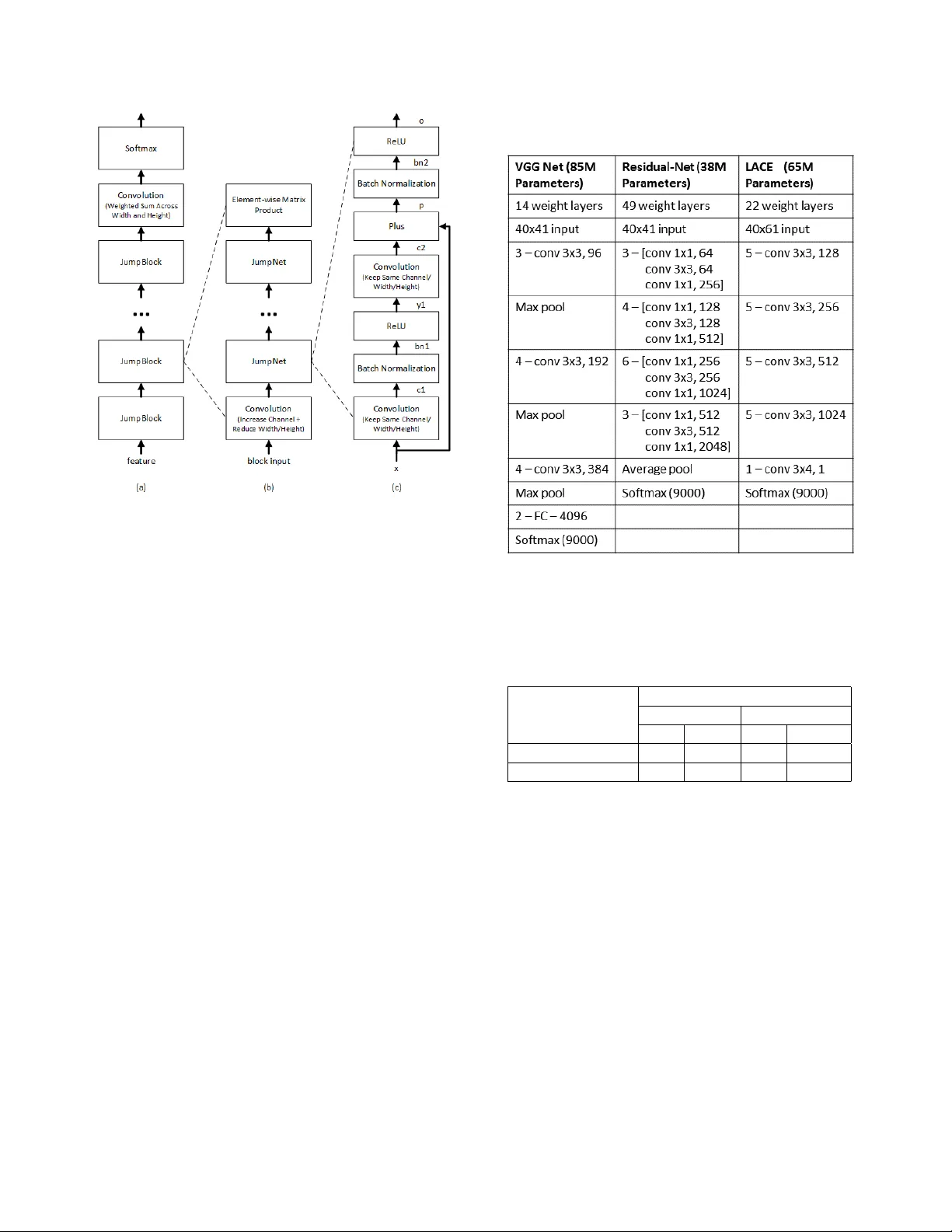
A CHIEVING HUMAN P ARITY IN CONVERSA TIONAL SPEECH RECOGNITION W . Xiong, J . Dr oppo, X. Huang, F . Seide, M. Seltzer , A. Stolc ke , D. Y u and G. Zweig Microsoft Research T echnical Report MSR-TR-2016-71 Re vised February 2017 ABSTRA CT Con versational speech recognition has served as a flagship speech recognition task since the release of the Switchboard corpus in the 1990s. In this paper, we measure the human er- ror rate on the widely used NIST 2000 test set, and find that our latest automated system has reached human parity . The error rate of professional transcribers is 5.9% for the Switch- board portion of the data, in which newly acquainted pairs of people discuss an assigned topic, and 11.3% for the CallHome portion where friends and family members hav e open-ended con versations. In both cases, our automated system estab- lishes a ne w state of the art, and edges past the human bench- mark, achieving error rates of 5.8% and 11.0%, respectively . The key to our system’ s performance is the use of various con v olutional and LSTM acoustic model architectures, com- bined with a novel spatial smoothing method and lattice-free MMI acoustic training, multiple recurrent neural network lan- guage modeling approaches, and a systematic use of system combination. Index T erms — Con versational speech recognition, con- volutional neural networks, recurrent neural networks, VGG, ResNet, LA CE, BLSTM, spatial smoothing. 1. INTR ODUCTION Recent years ha ve seen human performance lev els reached or surpassed in tasks ranging from the games of chess and Go [1, 2] to simple speech recognition tasks like carefully read newspaper speech [3] and rigidly constrained small- vocab ulary tasks in noise [4, 5]. In the area of speech recog- nition, much of the pioneering early work was dri ven by a series of carefully designed tasks with DARP A-funded datasets publicly released by the LDC and NIST [6]: first simple ones like the “resource management” task [7] with a small vocabulary and carefully controlled grammar; then read speech recognition in the W all Street Journal task [8]; then Broadcast Ne ws [9]; each progressi vely more difficult for automatic systems. One of last big initiatives in this area was in con versational telephone speech (CTS), which is especially difficult due to the spontaneous (neither read nor planned) nature of the speech, its informality , and t he self-corrections, hesitations and other disfluencies that are pervasi ve. The Switchboard [10] and later Fisher [11] data collections of the 1990s and early 2000s provide what is to date the largest and best studied of the con versational corpora. The history of work in this area includes ke y contributions by institutions such as IBM [12], BBN [13], SRI [14], A T&T [15], LIMSI [16], Cambridge Univ ersity [17], Microsoft [18] and numerous others. In the past, human performance on this task has been widely cited as being 4% [19]. Howe ver , the error rate estimate in [19] is attrib uted to a “personal communication, ” and the actual source of this number is ephemeral. T o better understand human performance, we hav e used professional transcribers to transcribe the actual test sets that we are working with, specifically the CallHome and Switchboard portions of the NIST ev al 2000 test set. W e find that the human error rates on these two parts are different almost by a factor of tw o, so a single number is inappropriate to cite. The error rate on Switchboard is about 5.9%, and for CallHome 11.3%. W e improve on our recently reported con versational speech recognition system [20] by about 0.4%, and now exceed human performance by a small margin. Our progress is a result of the careful engineering and optimization of conv olutional and recurrent neural net- works. While the basic structures ha ve been well kno wn for a long period [21, 22, 23, 24, 25, 26, 27], it is only recently that they hav e dominated the field as the best models for speech recognition. Surprisingly , this is the case for both acoustic modeling [28, 29, 30, 31, 32, 33] and language modeling [34, 35, 36, 37]. In comparison to the standard feed-forward MLPs or DNNs that first demonstrated breakthrough per - formance on conv ersational speech recognition [18], these acoustic models have the ability to model a large amount of acoustic context with temporal inv ariance, and in the case of con v olutional models, with frequency in variance as well. In language modeling, recurrent models appear to improv e over classical N-gram models through the use of an unbounded word history , as well as the generalization ability of contin- uous word representations [38]. In the meantime, ensemble learning has become commonly used in several neural mod- els [39, 40, 35], to improve robustness by reducing bias and variance. This paper is an expanded version of [20], with the following additional material: 1. A comprehensi ve assessment of human performance on the NIST ev al 2000 test set 2. The description of a nov el spatial regularization method which significantly boosts our LSTM acoustic model performance 3. The use of LSTM rather than RNN-LMs, and the use of a letter-trigram input representation 4. A two-le vel system combination, based on a subsystem of BLSTM-system variants that, by itself, surpasses the best previously reported results 5. Expanded coverage of the Microsoft Cognitiv e T oolkit (CNTK) used to build our models 6. An analysis of human v ersus machine errors, which indicates substantial equi valence, with the exception of the word classes of backchannel acknowledgments (e.g. “uh-huh”) and hesitations (e.g. “um”). The remainder of this paper describes our system in detail. Section 2 describes our measurement of human performance. Section 3 describes the conv olutional neural net (CNN) and long-short-term memory (LSTM) models. Section 4 de- scribes our implementation of i-v ector adaptation. Section 5 presents out lattice-free MMI training process. Language model rescoring is a significant part of our system, and de- scribed in Section 6. W e describe the CNTK toolkit that forms the basis of our neural network models in Section 7. Experimental results are presented in Section 8, followed by an error analysis in section 9, a revie w of relev ant prior work in 10 and concluding remarks. 2. HUMAN PERFORMANCE T o measure human performance, we le veraged an existing pipeline in which Microsoft data is transcribed on a weekly basis. This pipeline uses a large commercial vendor to per- form two-pass transcription. In the first pass, a transcriber works from scratch to transcribe the data. In the second pass, a second listener monitors the data to do error correction. Dozens of hours of test data are processed in each batch. One week, we added the NIST 2000 CTS ev aluation data to the work-list, without further comment. The intention was to measure the error rate of professional transcribers going about their normal ev eryday business. Aside from the standard two- pass checking in place, we did not do a complex multi-party transcription and adjudication process. The transcribers were giv en the same audio se gments as were provided to the speech recognition system, which results in short sentences or sen- tence fragments from a single channel. This makes the task easier since the speakers are more clearly separated, and more difficult since the two sides of the con versation are not in- terleav ed. Thus, it is the same condition as reported for our automated systems. The resulting numbers are 5.9% for the Switchboard portion, and 11.3% for the CallHome portion of the NIST 2000 test set, using the NIST scoring protocol. These numbers should be taken as an indication of the “error rate” of a trained professional working in industry-standard speech transcript production. (W e have submitted the human transcripts thus produced to the Linguistic Data Consortium for publication, so as to facilitate research by other groups.) Past work [41] reports inter -transcriber error rates for data taken from the later R T03 test set (which contains Switch- board and Fisher, but no CallHome data). Error rates of 4.1 to 4.5% are reported for e xtremely careful multiple transcrip- tions, and 9.6% for “quick transcriptions. ” While this is a different test set, the numbers are in line with our findings. W e note that the bulk of the Fisher training data, and the b ulk of the data overall, w as transcribed with the “quick transcrip- tion” guidelines. Thus, the current state of the art is actually far exceeding the noise le vel in its o wn training data. Per- haps the most important point is the e xtreme variability be- tween the two test subsets. The more informal CallHome data has almost double the human error rate of the Switchboard data. Interestingly , the same informality , multiple speakers per channel, and recording conditions that mak e CallHome hard for computers make it difficult for people as well. No- tably , the performance of our artificial system aligns almost exactly with the performance of people on both sets. 3. CONV OLUTIONAL AND LSTM NEURAL NETWORKS 3.1. CNNs W e use three CNN v ariants. The first is the VGG architecture of [42]. Compared to the networks used previously in image recognition, this network uses small (3x3) filters, is deeper , and applies up to five con volutional layers before pooling. The second network is modeled on the ResNet architecture [43], which adds highway connections [44], i.e. a linear trans- form of each layer’ s input to the layer’ s output [44, 45]. The only difference is that we apply Batch Normalization before computing ReLU acti v ations. The last CNN v ariant is the LA CE (layer-wise context expansion with attention) model [46]. LA CE is a TDNN [23] variant in which each higher layer is a weighted sum of nonlinear transformations of a win- dow of lower layer frames. In other words, each higher layer exploits broader context than lower layers. Lower layers fo- cus on extracting simple local patterns while higher layers extract complex patterns that co ver broader conte xts. Since not all frames in a window carry the same importance, an at- tention mask is applied. The LACE model dif fers from the earlier TDNN models e.g. [23, 47] in the use of a learned attention mask and ResNet like linear pass-through. As illus- trated in detail in Figure 1, the model is composed of four blocks, each with the same architecture. Each block starts Fig. 1 . LACE netw ork architecture with a con volution layer with stride 2 which sub-samples the input and increases the number of channels. This layer is followed by four RELU-con volution layers with jump links similar to those used in ResNet. T able 1 compares the layer structure and parameters of the three CNN architectures. W e also trained a fused model by combining a ResNet model and a V GG model at the senone posterior level. Both base models are independently trained, and then the score fusion weight is optimized on dev elopment data. The fused system is our best single system. 3.2. LSTMs While our best performing models are con volutional, the use of long short-term memory netw orks (LSTMs) is a close sec- ond. W e use a bidirectional architecture [48] without frame- skipping [29]. The core model structure is the LSTM defined in [28]. W e found that using networks with more than six layers did not improve the word error rate on the dev elop- ment set, and chose 512 hidden units, per direction, per layer , as that provided a reasonable trade-off between training time and final model accuracy . 3.3. Spatial Smoothing Inspired by the human auditory cortex, where neighboring neurons tend to simultaneously activ ate, we employ a spatial smoothing technique to improv e the accuracy of our LSTM models. The smoothing is implemented as a regulariza- tion term on the activ ations between layers of the acoustic T able 1 . Comparison of CNN architectures T able 2 . Accuracy improvements from spatial smoothing on the NIST 2000 CTS test set. The model is a six layer BLSTM, using i-vectors and 40 dimensional filterbank features, and a dimension of 512 in each direction of each layer . Model WER (%) 9000 senones 27000 senones CH SWB CH SWB Baseline 21.4 9.9 20.5 10.6 Spatial smoothing 19.2 9.3 19.5 9.2 model. First, each vector of acti v ations is re-interpreted as a 2-dimensional image. For example, if there are 512 neu- rons, they are interpreted as the pixels of a 16 by 32 image. Second, this image is high-pass filtered. The filter is imple- mented as a circular con volution with a 3 by 3 kernel. The center tap of the kernel has a value of 1 , and the remaining eight having a value of − 1 / 8 . Third, the energy of this high- pass filtered image is computed and added to the training objectiv e function. W e hav e found empirically that a suitable scale for this energy is 0 . 1 with respect to the existing cross entropy objective function. The ov erall effect of this process is to make the training algorithm prefer models that ha ve correlated neurons, and to improve the word error rate of the acoustic model. T able 2 shows the benefit in error rate for some of our early systems. W e observed error reductions of between 5 and 10% relativ e from spatial smoothing. 4. SPEAKER AD APTIVE MODELING Speaker adaptiv e modeling in our system is based on con- ditioning the network on an i-vector [49] characterization of each speaker [50, 51]. A 100-dimensional i-vector is gener- ated for each con versation side. For the LSTM system, the con versation-side i-vector v s is appended to each frame of input. For con v olutional networks, this approach is inappro- priate because we do not expect to see spatially contiguous patterns in the input. Instead, for the CNNs, we add a learn- able weight matrix W l to each layer, and add W l v s to the activ ation of the layer before the nonlinearity . Thus, in the CNN, the i-vector essentially serves as an speaker-dependent bias to each layer . Note that the i-vectors are estimated us- ing MFCC features; by using them subsequently in systems based on log-filterbank features, we may benefit from a form of feature combination. Performance improvements from i- vectors are shown in T able 3. The full experimental setup is described in Section 8. 5. LA TTICE-FREE SEQUENCE TRAINING After standard cross-entropy training, we optimize the model parameters using the maximum mutual information (MMI) objectiv e function. Denoting a w ord sequence by w and its corresponding acoustic realization by a , the training criterion is X w,a ∈ data log P ( w ) P ( a | w ) P 0 w P ( w 0 ) P ( a | w 0 ) . As noted in [52, 53], the necessary gradient for use in back- propagation is a simple function of the posterior probability of a particular acoustic model state at a gi ven time, as computed by summing over all possible word sequences in an uncon- strained manner . As first done in [12], and more recently in [54], this can be accomplished with a straightforward alpha- beta computation ov er the finite state acceptor representing the decoding search space. In [12], the search space is taken to be an acceptor representing the composition H C LG for a un- igram language model L on w ords. In [54], a language model on phonemes is used instead. In our implementation, we use a mixed-history acoustic unit language model. In this model, the probability of transitioning into a new context-dependent phonetic state (senone) is conditioned on both the senone and phone history . W e found this model to perform better than either purely word-based or phone-based models. Based on a set of initial experiments, we dev eloped the following proce- dure: 1. Perform a forced alignment of the training data to select lexical v ariants and determine frame-aligned senone se- quences. 2. Compress consecutiv e framewise occurrences of a sin- gle senone into a single occurrence. 3. Estimate an unsmoothed, variable-length N-gram lan- guage model from this data, where the history state con- sists of the previous phone and previous senones within the current phone. T o illustrate this, consider the sample senone sequence { s s2.1288, s s3.1061, s s4.1096 } , { eh s2.527, eh s3.128, eh s4.66 } , { t s2.729, t s3.572, t s4.748 } . When predict- ing the state following eh s4.66 the history consists of ( s , eh s2.527, eh s3.128, eh s4.66), and following t s2.729, the history is ( eh , t s2.729). W e construct the denominator graph from this language model, and HMM transition probabilities as determined by transition-counting in the senone sequences found in the training data. Our approach not only lar gely reduces the complexity of b uilding up the language model but also provides very reliable training performance. W e hav e found it con venient to do the full computation, with- out pruning, in a series of matrix-vector operations on the GPU. The underlying acceptor is represented with a sparse matrix, and we maintain a dense likelihood vector for each time frame. The alpha and beta recursions are implemented with CUSP ARSE level-2 routines: sparse-matrix, dense vec- tor multiplies. Run time is about 100 times faster than real time. As in [54], we use cross-entropy regularization. In all the lattice-free MMI (LFMMI) experiments mentioned belo w we use a trigram language model. Most of the gain is usually obtained after processing 24 to 48 hours of data. 6. LM RESCORING AND SYSTEM COMBINA TION An initial decoding is done with a WFST decoder, using the architecture described in [55]. W e use an N-gram lan- guage model trained and pruned with the SRILM toolkit [56]. The first-pass LM has approximately 15.9 million bi- grams, trigrams, and 4grams, and a v ocabulary of 30,500 words. It gi ves a perple xity of 69 on the 1997 CTS e valuation transcripts. The initial decoding produces a lattice with the pronunciation variants marked, from which 500-best lists are generated for rescoring purposes. Subsequent N-best rescor- ing uses an unpruned LM comprising 145 million N-grams. All N-gram LMs were estimated by a maximum entropy cri- terion as described in [57]. The N-best hypotheses are then rescored using a combination of the lar ge N-gram LM and sev eral neural net LMs. W e ha ve experimented with both RNN LMs and LSTM LMs, and describe the details in the following tw o sections. 6.1. RNN-LM setup Our RNN-LMs are trained and ev aluated using the CUED- RNNLM toolkit [58]. Our RNN-LM configuration has sev- eral distinctiv e features, as described belo w . 1. W e trained both standard, forward-predicting RNN- LMs and backw ard RNN-LMs that predict words in T able 3 . Performance improv ements from i-vector and LFMMI training on the NIST 2000 CTS test set Configuration WER (%) ReLU-DNN ResNet-CNN BLSTM LA CE CH SWB CH SWB CH SWB CH SWB Baseline 21.9 13.4 17.5 11.1 17.3 10.3 16.9 10.4 i-vector 20.1 11.5 16.6 10.0 17.6 9.9 16.4 9.3 i-vector+LFMMI 17.9 10.2 15.2 8.6 16.3 8.9 15.2 8.5 rev erse temporal order . The log probabilities from both models are added. 2. As is customary , the RNN-LM probability estimates are interpolated at the word-lev el with corresponding N- gram LM probabilities (separately for the forward and backward models). In addition, we trained a second RNN-LM for each direction, obtained by starting with different random initial weights. The two RNN-LMs and the N-gram LM for each direction are interpolated with weights of (0.375, 0.375, 0.25). 3. In order to make use of LM training data that is not fully matched to the target con versational speech domain, we start RNN-LM training with the union of in-domain (here, CTS) and out-of-domain (e.g., W eb) data. Upon con ver gence, the network undergoes a second training phase using the in-domain data only . Both training phases use in-domain validation data to re gulate the learning rate schedule and termination. Because the size of the out-of-domain data is a multiple of the in- domain data, a standard training on a simple union of the data would not yield a well-matched model, and hav e poor perplexity in the tar get domain. 4. W e found best results with an RNN-LM configuration that had a second, non-recurrent hidden layer . This pro- duced lo wer perplexity and word error than the stan- dard, single-hidden-layer RNN-LM architecture [34]. 1 The ov erall network architecture thus had two hidden layers with 1000 units each, using ReLU nonlineari- ties. T raining used noise-contrastiv e estimation (NCE) [59]. 5. The RNN-LM output vocab ulary consists of all words occurring more than once in the in-domain training set. While the RNN-LM estimates a probability for un- known words, we take a different approach in rescor- ing: The number of out-of-set words is recorded for each hypothesis and a penalty for them is estimated for them when optimizing the relative weights for all model scores (acoustic, LM, pronunciation), using the SRILM nbest-optimize tool. 1 Howe ver , adding more hidden layers produced no further gains. 6.2. LSTM-LM setup After obtaining good results with RNN-LMs we also explored the LSTM recurrent network architecture for language mod- eling, inspired by recent w ork sho wing gains o ver RNN-LMs for con versational speech recognition [37]. In addition to ap- plying the lessons learned from our RNN-LM experiments, we explored additional alternati ves, as described belo w . 1. There are tw o types of input v ectors our LSTM LMs take, word based one-hot v ector input and letter trigram vector [60] input. Including both forward and back- ward models, we trained four dif ferent LSTM LMs in total. 2. For the word based input, we lev eraged the approach from [61] to tie the input embedding and output em- bedding together . 3. Here we also used a two-phase training schedule to train the LSTM LMs. First we train the model on the combination of in-domain and out-domain data for four data passes without any learning rate adjustment. W e then start from the resulting model and train on in-domain data until con ver gence. 4. Overall the letter trigram based models perform a little better than the word based language model. W e tried applying dropout on both types of language models but didn’t see an impro vement. 5. Con vergence w as improv ed through a v ariation of self- stabilization [62], in which each output vector x of non- linearities are scaled by 1 4 ln(1 + e 4 β ) , where a β is a scalar that is learned for each output. This has a similar effect as the scale of the well-known batch normaliza- tion technique, but can be used in recurrent loops. 6. T able 4 shows the impact of number of layers on the fi- nal perplexities. Based on this, we proceeded with three hidden layers, with 1000 hidden units each. The per- plexities of each LSTM-LM we used in the final com- bination (before interpolating with the N-gram model) can be found in T able 5. For the final system, we interpolated two LSTM-LMs with an N-gram LM for the forward-direction LM, and similarly for the backward-direction LM. All LSTMs use three hidden T able 4 . LSTM perplexities (PPL) as a function of hidden layers, trained on in-domain data only , computed on 1997 CTS ev al transcripts. Language model PPL letter trigram input with one layer (baseline) 63.2 + two hidden layers 61.8 + three hidden layers 59.1 + four hidden layers 59.6 + fiv e hidden layers 60.2 + six hidden layers 63.7 T able 5 . Perplexities (PPL) of the four LSTM LMs used in the final combination. PPL is computed on 1997 CTS e val transcripts. All the LSTM LMs are with three hidden layers. Language model PPL RNN: 2 layers + word input (baseline) 59.8 LSTM: word input in forward direction 54.4 LSTM: word input in backward direction 53.4 LSTM: letter trigram input in forward direction 52.1 LSTM: letter trigram input in backward direction 52.0 layers and are trained on in-domain and web data. Unlike for the RNN-LMs, the two models being interpolated differ not just in their random initialization, b ut also in the input encod- ing (one uses a triletter encoding, the other a one-hot word encoding). The forward and backward LM log probability scores are combined additiv ely . 6.3. T raining data The 4-gram language model for decoding was trained on the av ailable CTS transcripts from the D ARP A EARS program: Switchboard (3M words), BBN Switchboard-2 transcripts (850k), Fisher (21M), English CallHome (200k), and the Uni- T able 6 . Performance of various v ersions of neural-net-based LM rescoring. Perplexities (PPL) are computed on 1997 CTS ev al transcripts; word error rates (WER) on the NIST 2000 Switchboard test set. Language model PPL WER 4-gram LM (baseline) 69.4 8.6 + RNNLM, CTS data only 62.6 7.6 + W eb data training 60.9 7.4 + 2nd hidden layer 59.0 7.4 + 2-RNNLM interpolation 57.2 7.3 + backward RNNLMs - 6.9 + LSTM-LM, CTS + W eb data 51.4 6.9 + 2-LSTM-LM interpolation 50.5 6.8 + backward LSTM-LM - 6.6 versity of W ashington con versational W eb corpus (191M). A separate N-gram model was trained from each source and interpolated with weights optimized on R T -03 transcripts. For the unpruned large rescoring 4-gram, an additional LM component was added, trained on 133M w ord of LDC Broad- cast News texts. The N-gram LM configuration is modeled after that described in [51], e xcept that max ent smoothing was used. The RNN and LSTM LMs were trained on Switch- board and Fisher transcripts as in-domain data (20M words for gradient computation, 3M for v alidation). T o this we added 62M words of UW W eb data as out-of-domain data, for use in the two-phase training procedure described abov e. 6.4. RNN-LM and LSTM-LM performance T able 6 gives perplexity and word error performance for vari- ous recurrent neural net LM setups, from simple to more com- plex. The acoustic model used was the ResNet CNN. Note that, unlike the results in T ables 4 and 5, the neural net LMs in T able 6 are interpolated with the N-gram LM. As can be seen, each of the measures described earlier adds incremen- tal gains, which, howe ver , add up to a substantial improve- ment ov erall. The total g ain relativ e to a purely N-gram based system is a 20% relativ e error reduction with RNN-LMs, and 23% with LSTM-LMs. As sho wn later (see T able 8) the gains with different acoustic models are similar . 6.5. System Combination The LM rescoring is carried out separately for each acoustic model. The rescored N-best lists from each subsystem are then aligned into a single confusion network [63] using the SRILM nbest-r over tool. Ho wev er , the number of potential candidate systems is too large to allow an all-out combina- tion, both for practical reasons and due to overfitting issues. Instead, we perform a greedy search, starting with the single best system, and successi vely adding additional systems, to find a small set of systems that are maximally complemen- tary . The R T -02 Switchboard set was used for this search pro- cedure. W e experimented with two search algorithms to find good subsets of systems. W e alw ays start with the system giving the best indi vidual accuracy on the dev elopment set. In one approach, a greedy forward search then adds systems incrementally to the combination, giving each equal weight. If no improvement is found with any of the unused systems, we try adding each with successiv ely lower relativ e weights of 0.5, 0.2, and 0.1, and stop if none of these giv e an impro ve- ment. A second variant of the search procedure that can giv e lower error (as measured on the de vset) estimates the best sys- tem weights for each incremental combination candidate. The weight estimation is done using an e xpectation-maximization algorithm based on aligning the reference words to the con- fusion networks, and maximizing the weighted probability of the correct word at each alignment position. T o av oid ov erfit- ting, the weights for an N -way combination are smoothed hi- erarchically , i.e., interpolated with the weights from the ( N − 1) -way system that preceded it. This tends to giv e robust weights that are biased toward the early (i.e., better) subsys- tems. The final system incorporated a v ariety of BLSTM models with roughly similar performance, but dif fering in various metaparameters (number of senones, use of spatial smoothing, and choice of pronunciation dictionaries). 2 T o further limit the number of free parameters to be estimated i n system combination, we performed system selection in two stages. First, we selected the four best BLSTM systems. W e then combined these with equal weights and treated them as a single subsystem in searching for a larger combination in- cluding other acoustic models. This yielded our best ov erall combined system, as reported in Section 8.3. 7. MICR OSOFT COGNITIVE TOOLKIT (CNTK) All neural networks in the final system were trained with the Microsoft Cognitive T oolkit, or CNTK [64, 65]. on a Linux-based multi-GPU server farm. CNTK allows for flex- ible model definition, while at the same time scaling v ery efficiently across multiple GPUs and multiple servers. The resulting f ast experimental turnaround using the full 2000- hour corpus was critical for our work. 7.1. Flexible, T erse Model Definition In CNTK, a neural network (and the training criteria) are specified by its formula, using a custom functional lan- guage (BrainScript), or Python. A graph-based execution engine, which provides automatic differentiation, then trains the model’ s parameters through SGD. Lev eraging a stock li- brary of common layer types, networks can be specified very tersely . Samples can be found in [64]. 7.2. Multi-Server T raining using 1-bit SGD T raining the acoustic models in this paper on a single GPU would take many weeks or ev en months. CNTK made train- ing times feasible by parallelizing the SGD training with our 1-bit SGD parallelization technique [66]. This data-parallel method distributes minibatches over multiple worker nodes, and then aggregates the sub-gradients. While the necessary communication time would otherwise be prohibiti ve, the 1- bit SGD method eliminates the bottleneck by two techniques: 1-bit quantization of gradients and automatic minibatch-size scaling . In [66], we sho wed that gradient v alues can be quan- tized to just a single bit, if one carries over the quantization er- ror from one minibatch to the next. Each time a sub-gradient is quantized, the quantization error is computed and remem- bered, and then added to the ne xt minibatch’ s sub-gradient. 2 W e used two different dictionaries, one based on a standard phone set and another with dedicated vo wel and nasal phones used only in the pro- nunciations of filled pauses (“uh”, “um”) and backchannel ackno wledgments (“uh-huh”, “mhm”), similar to [63]. This reduces the required bandwidth 32-fold with minimal loss in accuracy . Secondly , automatic minibatch-size scaling progressiv ely decreases the frequency of model updates. At regular intervals (e.g. ev ery 72h of training data), the trainer tries larger minibatch sizes on a small subset of data and picks the largest that maintains training loss. These two techniques allow for excellent multi-GPU/server scalability , and reduced the acoustic-model training times on 2000h from months to between 1 and 3 weeks, making this work feasible. 7.3. Computational performance T able 7 compares the runtimes, as multiples of speech dura- tion, of various processing steps associated with the differ - ent acoustic model architectures (figures for DNNs are giv en only as a reference point, since they are not used in our sys- tem). Acoustic model (AM) training comprises the forward and backward dynamic programming passes, as well as pa- rameter updates. AM ev aluation refers to the forward com- putation only . Decoding includes AM ev aluation along with hypothesis search (only the former mak es use of the GPU). Runtimes were measured on a 12-core Intel Xeon E5-2620v3 CPU clocked at 2.4GHz, with an Nvidia T itan X GPU. W e observe that the GPU gives a 10 to 100-fold speedup for AM ev aluation over the CPU implementation. AM e v aluation is thus reduced to a small faction of ov erall decoding time, mak- ing near-realtime operation possible. 8. EXPERIMENTS AND RESUL TS 8.1. Speech corpora W e train with the commonly used English CTS (Switchboard and Fisher) corpora. Ev aluation is carried out on the NIST 2000 CTS test set, which comprises both Switchboard (SWB) and CallHome (CH) subsets. The w av eforms were segmented according to the NIST partitioned e v aluation map (PEM) file, with 150ms of dithered silence padding added in the case of the CallHome con versations. 3 The Switchboard-1 portion of the NIST 2002 CTS test set was used for tuning and de velop- ment. The acoustic training data is comprised by LDC cor- pora 97S62, 2004S13, 2005S13, 2004S11 and 2004S09; see [12] for a full description. 8.2. Acoustic Model Details Forty-dimensional log-filterbank features were extracted ev- ery 10 milliseconds, using a 25-millisecond analysis windo w . The CNN models used window sizes as indicated in T able 1, and the LSTMs processed one frame of input at a time. The bulk of our models use three state left-to-right triphone mod- els with 9000 tied states. Additionally , we hav e trained sev- eral models with 27k tied states. The phonetic inv entory in- 3 Using the sox tool options pad 0.15 0.15 dither -p 14 . T able 7 . Runtimes as factor of speech duration for various aspects of acoustic modeling and decoding, for different types of acoustic model Processing step Hardware DNN ResNet-CNN BLSTM LA CE AM training GPU 0.012 0.60 0.022 0.23 AM ev aluation GPU 0.0064 0.15 0.0081 0.081 AM ev aluation CPU 0.052 11.7 n/a 8.47 Decoding GPU 1.04 1.19 1.40 1.38 T able 8 . W ord error rates (%) on the NIST 2000 CTS test set with different acoustic models. Unless otherwise noted, models are trained on the full 2000 hours of data and hav e 9k senones. Model N-gram LM RNN-LM LSTM-LM CH SWB CH SWB CH SWB ResNet, 300h training 19.2 10.0 17.7 8.2 17.0 7.7 ResNet 14.8 8.6 13.2 6.9 12.5 6.6 ResNet, GMM alignments 15.3 8.8 13.7 7.3 12.8 6.9 VGG 15.7 9.1 14.1 7.6 13.2 7.1 VGG + ResNet 14.5 8.4 13.0 6.9 12.2 6.4 LA CE 15.0 8.4 13.5 7.2 13.0 6.7 BLSTM 16.5 9.0 15.2 7.5 14.4 7.0 BLSTM, spatial smoothing 15.4 8.6 13.7 7.4 13.0 7.0 BLSTM, spatial smoothing, 27k senones 15.3 8.3 13.8 7.0 13.2 6.8 BLSTM, spatial smoothing, 27k senones, alternate dictionary 14.9 8.3 13.7 7.0 13.0 6.7 BLSTM system combination 13.2 7.3 12.1 6.4 11.6 6.0 Full system combination 13.0 7.3 11.7 6.1 11.0 5.8 T able 9 . Comparativ e error rates from the literature and hu- man error as measured in this work Model N-gram LM Neural net LM CH SWB CH SWB Pov ey et al. [54] LSTM 15.3 8.5 - - Saon et al. [51] LSTM 15.1 9.0 - - Saon et al. [51] system 13.7 7.6 12.2 6.6 2016 Microsoft system 13.3 7.4 11.0 5.8 Human transcription 11.3 5.9 cludes special models for noise, v ocalized-noise, laughter and silence. W e use a 30k-v ocab ulary derived from the most com- mon words in the Switchboard and Fisher corpora. The de- coder uses a statically compiled unigram graph, and dynam- ically applies the language model score. The unigram graph has about 300k states and 500k arcs. T able 3 sho ws the result of i-vector adaptation and LFMMI training on sev eral of our early systems. W e achiev e a 5–8% relative improv ement from i-vectors, including on CNN systems. The last ro w of T able 3 shows the effect of LFMMI training on the different models. W e see a consistent 7–10% further relativ e reduction in error rate for all models. Considering the great increase in procedu- ral simplicity of LFMMI over the pre vious practice of writing lattices and post-processing them, we consider LFMMI to be a significant advance in technology . 8.3. Overall Results and Discussion The performance of all our component models is shown in T able 8, along with the BLSTM combination and full system combination results. (Recall that the four best BLSTM sys- tems are combined with equal weights first, as described in Section 6.5.) Ke y benchmarks from the literature, our own best results, and the measured human error rates are com- pared in T able 9. 4 All models listed in T able 8 are selected for the combined systems for one or more of the three rescor- ing LMs. The only exception is the VGG+ResNet system, which combines acoustic senone posteriors from the V GG and ResNet networks. While this yields our single best acous- tic model, only the individual VGG and ResNet models are used in the overall system combination. W e also observe that the four model variants chosen for the combined BLSTM sub- system differ incrementally by one hyperparameter (smooth- 4 When comparing the last row in T able 3 with the “N-gram LM” results in T able 8, note that the former results were obtained with the pruned N-gram LM used in the decoder and fixed score weights (during lattice generation), whereas the latter results are from rescoring with the unpruned N-gram LM (during N-best generation), using optimized score weighting. Accordingly , the rescoring results are generally somewhat better . ing, number of senones, dictionary), and that the BLSTMs alone achieve an error that is within 3% relative of the full system combination. This validates the rationale that choos- ing different hyperparameters is an ef fecti ve way to obtain complementary systems for combination purposes. W e also assessed the lower bound of performance for our lattice/N- best rescoring paradigm. The 500-best lists from the lattices generated with the ResNet CNN system had an oracle (lo west achiev able) WER of 2.7% on the Switchboard portion of the NIST 2000 evaluation set, and an oracle WER of 4.9% on the CallHome portion. The oracle error of the combined system is even lower (though harder to quantify) since (1) N-best out- put from all systems are combined and (2) confusion network construction generates new possible hypotheses not contained in the original N-best lists. W ith oracle error rates less than half the currently achie ved actual error rates, we conclude that search errors are not a major limiting factor to ev en better ac- curacy . 9. ERR OR ANAL YSIS In this section, we compare the errors made by our artifi- cial recognizer with those made by human transcribers. W e find that the machine errors are substantially the same as human ones, with one large exception: confusions between backc hannel words and hesitations . The distinction is that backchannel words like “uh-huh” are an acknowledgment of the speak er , also signaling that the speaker should keep talking, while hesitations like “uh” are used to indicate that the current speaker has more to say and w ants to keep his or her turn. 5 As turn-management devices, these two classes of words therefore ha ve exactly opposite functions. T able 10 sho ws the ten most common substitutions for both hu- mans and the artificial system. T ables 11 and 12 do the same for deletions and insertions. F ocusing on the substitutions, we see that by far the most common error in the ASR sys- tem is the confusion of a hesitation in the reference for a backchannel in the hypothesis. People do not seem to have this problem. W e speculate that this is due to the nature of the Fisher training corpus, where the “quick transcription” guidelines were predominately used [41]. W e find that there is inconsistent treatment of backchannel and hesitation in the resulting data; the relatively poor performance of the au- tomatic system here might simply be due to confusions in the training data annotations. For perspective, there are over twenty-one thousand words in each test set. Thus the errors due to hesitation/backchannel substitutions account for an error rate of only about 0.2% absolute. The most frequent substitution for people on the Switch- board corpus was mistaking a hesitation in the reference for 5 The NIST scoring protocol treats hesitation words as optional, and we therefore delete them from our recognizer output prior to scoring. This ex- plains why we see many substitutions of backchannels for hesitations, but not vice-versa. the word “hmm. ” The scoring guidelines treat “hmm” as a word distinct from backchannels and hesitations, so this is not a scoring mistake. Examination of the contexts in which the error is made show that it is most often intended to acknowl- edge the other speaker , i.e. as a backchannel. For both people and our automated system, the insertion and deletion patterns are similar: short function words are by far the most frequent errors. In particular, the single most common error made by the transcribers was to omit the word “I. ” While we believe further improvement in function and content words is possi- ble, the significance of the remaining backchannel/hesitation confusions is unclear . T able 13 shows the overall error rates broken down by substitutions, insertions and deletions. W e see that the human transcribers hav e a somewhat lower sub- stitution rate, and a higher deletion rate. The relati vely higher deletion rate might reflect a human bias to a void outputting uncertain information, or the productivity demands on a pro- fessional transcriber . In all cases, the number of insertions is relativ ely small. 10. RELA TION TO PRIOR WORK Compared to earlier applications of CNNs to speech recog- nition [67, 68], our networks are much deeper , and use linear bypass connections across conv olutional layers. They are similar in spirit to those studied more recently by [31, 30, 51, 32, 33]. W e improv e on these architectures with the LA CE model [46], which iterati vely expands the ef fecti ve window size, layer -by-layer, and adds an attention mask to differentially weight distant context. Our spatial regulariza- tion technique is similar in spirit to stimulated deep neural networks [69]. Whereas stimulated networks use a supervi- sion signal to encourage locality of activ ations in the model, our technique is automatic. Our use of lattice-free MMI is distinctiv e, and extends previous work [12, 54] by proposing the use of a mixed triphone/phoneme history in the language model. On the language modeling side, we achiev e a per- formance boost by combining multiple LSTM-LMs in both forward and backward directions, and by using a two-phase training regimen to get best results from out-of-domain data. For our best CNN system, LSTM-LM rescoring yields a rela- tiv e word error reduction of 23%, and a 20% relati ve gain for the combined recognition system, considerably larger than previously reported for conv ersational speech recognition [37]. 11. CONCLUSIONS W e ha ve measured the human error rate on NIST’ s 2000 con- versational telephone speech recognition task. W e find that there is a great deal of variability between the Switchboard and CallHome subsets, with 5.8% and 11.0% error rates re- spectiv ely . For the first time, we report automatic recogni- tion performance on par with human performance on this task. T able 10 . Most common substitutions for ASR system and humans. The number of times each error occurs is followed by the word in the reference, and what appears in the hypothesis instead. CH SWB ASR Human ASR Human 45: (%hesitation) / %bcack 12: a / the 29: (%hesitation) / %bcack 12: (%hesitation) / hmm 12: was / is 10: (%hesitation) / a 9: (%hesitation) / oh 10: (%hesitation) / oh 9: (%hesitation) / a 10: was / is 9: was / is 9: was / is 8: (%hesitation) / oh 7: (%hesitation) / hmm 8: and / in 8: (%hesitation) / a 8: a / the 7: bentsy / bensi 6: (%hesitation) / i 5: in / and 7: and / in 7: is / was 6: in / and 4: (%hesitation) / %bcack 7: it / that 6: could / can 5: (%hesitation) / a 4: and / in 6: in / and 6: well / oh 5: (%hesitation) / yeah 4: is / was 5: a / to 5: (%hesitation) / %bcack 5: a / the 4: that / it 5: aw / oh 5: (%hesitation) / oh 5: jeez / jeeze 4: the / a T able 11 . Most common deletions for ASR system and hu- mans. CH SWB ASR Human ASR Human 44: i 73: i 31: it 34: i 33: it 59: and 26: i 30: and 29: a 48: it 19: a 29: it 29: and 47: is 17: that 22: a 25: is 45: the 15: you 22: that 19: he 41: %bcack 13: and 22: you 18: are 37: a 12: have 17: the 17: oh 33: you 12: oh 17: to 17: that 31: oh 11: are 15: oh 17: the 30: that 11: is 15: yeah Our system’ s performance can be attributed to the systematic use of LSTMs for both acoustic and language modeling, as well as CNNs in the acoustic model, and extensiv e combina- tion of complementary system for both acoustic and language modeling. Acknowledgments W e thank Arul Menezes for access to the Microsoft transcrip- tion pipeline; Chris Basoglu, Amit Agarwal and Marko Rad- milac for their inv aluable assistance with CNTK; Jinyu Li and Partha Parthasarathy for many helpful conv ersations. W e also thank X. Chen from Cambridge University for v aluable assis- tance with the CUED-RNNLM toolkit, and the International Computer Science Institute for compute and data resources. 12. REFERENCES [1] M. Campbell, A. J. Hoane, and F .-h. Hsu, “Deep Blue”, Artificial intelligence , v ol. 134, pp. 57–83, 2002. T able 12 . Most common insertions for ASR system and hu- mans. CH SWB ASR Human ASR Human 15: a 10: i 19: i 12: i 15: is 9: and 9: and 11: and 11: i 8: a 7: of 9: you 11: the 8: that 6: do 8: is 11: you 8: the 6: is 6: they 9: it 7: hav e 5: but 5: do 7: oh 5: you 5: yeah 5: hav e 6: and 4: are 4: air 5: it 6: in 4: is 4: in 5: yeah 6: know 4: they 4: you 4: a T able 13 . Overall substitution, deletion and insertion rates. CH SWB ASR Human ASR Human sub 6.5 4.1 3.3 2.6 del 3.3 6.5 1.8 2.7 ins 1.4 0.7 0.7 0.7 all 11.1 11.3 5.9 5.9 [2] D. Silver , A. Huang, C. J. Maddison, A. Guez, L. Sifre, G. V an Den Driessche, J. Schrittwieser , I. Antonoglou, V . Panneershelv am, M. Lanctot, et al., “Mastering the game of Go with deep neural networks and tree search”, Natur e , v ol. 529, pp. 484–489, 2016. [3] D. Amodei, R. Anubhai, E. Battenberg, C. Case, J. Casper , B. Catanzaro, J. Chen, M. Chrzanowski, A. Coates, G. Diamos, et al., “Deep Speech 2: End-to- end speech recognition in English and Mandarin”, arXiv preprint arXiv:1512.02595, 2015. [4] T . T . Kristjansson, J. R. Hershey , P . A. Olsen, S. J. Ren- nie, and R. A. Gopinath, “Super -human multi-talker speech recognition: the IBM 2006 Speech Separation Challenge system”, in Pr oc. Interspeech , vol. 12, p. 155, 2006. [5] C. W eng, D. Y u, M. L. Seltzer, and J. Droppo, “Single- channel mixed speech recognition using deep neural networks”, in Pr oc. IEEE ICASSP , pp. 5632–5636. IEEE, 2014. [6] D. S. Pallett, “ A look at NIST’ s benchmark ASR tests: past, present, and future”, in IEEE Automatic Speech Recognition and Understanding W orkshop , pp. 483– 488. IEEE, 2003. [7] P . Price, W . M. Fisher , J. Bernstein, and D. S. Pal- lett, “The D ARP A 1000-word resource management database for continuous speech recognition”, in Pr oc. IEEE ICASSP , pp. 651–654. IEEE, 1988. [8] D. B. Paul and J. M. Baker , “The design for the wall street journal-based csr corpus”, in Pr oceedings of the workshop on Speech and Natur al Language , pp. 357– 362. Association for Computational Linguistics, 1992. [9] D. Graf f, Z. W u, R. MacIntyre, and M. Liberman, “The 1996 broadcast ne ws speech and language-model cor- pus”, in Proceedings of the D ARP A W orkshop on Spo- ken Languag e technology , pp. 11–14, 1997. [10] J. J. Godfrey , E. C. Holliman, and J. McDaniel, “Switch- board: T elephone speech corpus for research and dev el- opment”, in Proc. IEEE ICASSP , vol. 1, pp. 517–520. IEEE, 1992. [11] C. Cieri, D. Miller, and K. W alker , “The Fisher corpus: a resource for the ne xt generations of speech-to-text”, in LREC , vol. 4, pp. 69–71, 2004. [12] S. F . Chen, B. Kingsb ury , L. Mangu, D. Po ve y , G. Saon, H. Soltau, and G. Zweig, “ Adv ances in speech transcrip- tion at IBM under the DARP A EARS program”, IEEE T rans. Audio, Speech, and Languag e Pr ocessing , vol. 14, pp. 1596–1608, 2006. [13] S. Matsoukas, J.-L. Gauvain, G. Adda, T . Colthurst, C.- L. Kao, O. Kimball, L. Lamel, F . Lefevre, J. Z. Ma, J. Makhoul, et al., “ Adv ances in transcription of broad- cast news and con versational telephone speech within the combined ears bbn/limsi system”, IEEE T ransac- tions on Audio, Speech, and Language Pr ocessing , vol. 14, pp. 1541–1556, 2006. [14] A. Stolcke, B. Chen, H. Franco, V . R. R. Gadde, M. Graciarena, M.-Y . Hwang, K. Kirchhoff, A. Man- dal, N. Morgan, X. Lei, et al., “Recent innov ations in speech-to-text transcription at SRI-ICSI-UW”, IEEE T ransactions on Audio, Speech, and Languag e Pr ocess- ing , vol. 14, pp. 1729–1744, 2006. [15] A. Ljolje, “The A T&T 2001 L VCSR system”, NIST L VCSR W orkshop, 2001. [16] J.-L. Gauvain, L. Lamel, H. Schwenk, G. Adda, L. Chen, and F . Lefe vre, “Con versational telephone speech recognition”, in Pr oc. IEEE ICASSP , vol. 1, pp. I–212. IEEE, 2003. [17] G. Ev ermann, H. Y . Chan, M. J. F . Gales, T . Hain, X. Liu, D. Mrva, L. W ang, and P . C. W oodland, “De- velopment of the 2003 cu-htk conv ersational telephone speech transcription system”, in Pr oc. IEEE ICASSP , vol. 1, pp. I–249. IEEE, 2004. [18] F . Seide, G. Li, and D. Y u, “Con versational speech transcription using context-dependent deep neural net- works”, in Pr oc. Interspeech , pp. 437–440, 2011. [19] R. P . Lippmann, “Speech recognition by machines and humans”, Speech Communication , v ol. 22, pp. 1–15, 1997. [20] W . Xiong, J. Droppo, X. Huang, F . Seide, M. Seltzer, A. Stolcke, D. Y u, and G. Zweig, “The Mi- crosoft 2016 con versational speech recognition sys- tem”, submitted to ICASSP , 2017, preprint at https://arxiv .org/abs/1609.03528. [21] F . J. Pineda, “Generalization of back-propagation to re- current neural networks”, Physical Review Letters , vol. 59, pp. 2229, 1987. [22] R. J. W illiams and D. Zipser , “ A learning algorithm for continually running fully recurrent neural networks”, Neural Computation , v ol. 1, pp. 270–280, 1989. [23] A. W aibel, T . Hanazawa, G. Hinton, K. Shikano, and K. J. Lang, “Phoneme recognition using time-delay neu- ral networks”, IEEE T rans. Acoustics, Speech, and Sig- nal Pr ocessing , vol. 37, pp. 328–339, 1989. [24] Y . LeCun and Y . Bengio, “Con volutional networks for images, speech, and time series”, The handbook of brain theory and neural networks , v ol. 3361, pp. 1995, 1995. [25] Y . LeCun, B. Boser , J. S. Denker , D. Henderson, R. E. How ard, W . Hubbard, and L. D. Jackel, “Backpropaga- tion applied to handwritten zip code recognition”, Neu- ral computation , v ol. 1, pp. 541–551, 1989. [26] T . Robinson and F . Fallside, “ A recurrent error propa- gation network speech recognition system”, Computer Speech & Languag e , vol. 5, pp. 259–274, 1991. [27] S. Hochreiter and J. Schmidhuber , “Long short-term memory”, Neural Computation , vol. 9, pp. 1735–1780, 1997. [28] H. Sak, A. W . Senior , and F . Beaufays, “Long short- term memory recurrent neural network architectures for large scale acoustic modeling”, in Proc. Interspeech , pp. 338–342, 2014. [29] H. Sak, A. Senior, K. Rao, and F . Beaufays, “Fast and accurate recurrent neural network acoustic models for speech recognition”, in Pr oc. Interspeech , pp. 1468– 1472, 2015. [30] G. Saon, H.-K. J. K uo, S. Rennie, and M. Picheny , “The IBM 2015 English conv ersational telephone speech recognition system”, in Interspeec h , pp. 3140–3144, 2015. [31] T . Sercu, C. Puhrsch, B. Kingsb ury , and Y . LeCun, “V ery deep multilingual conv olutional neural networks for L VCSR”, in Proc. IEEE ICASSP , pp. 4955–4959. IEEE, 2016. [32] M. Bi, Y . Qian, and K. Y u, “V ery deep con volutional neural networks for L VCSR”, in Proc. Interspeech , pp. 3259–3263, 2015. [33] Y . Qian, M. Bi, T . T an, and K. Y u, “V ery deep con v olu- tional neural networks for noise robust speech recogni- tion”, IEEE/ACM T rans. Audio, Speech, and Language Pr ocessing , vol. 24, pp. 2263–2276, Aug. 2016. [34] T . Mikolo v , M. Karafi ´ at, L. Burget, J. Cernock ` y, and S. Khudanpur , “Recurrent neural network based lan- guage model”, in Proc. Interspeec h , pp. 1045–1048, 2010. [35] T . Mikolov and G. Zweig, “Context dependent recurrent neural network language model”, in Pr oc. Interspeech , pp. 901–904, 2012. [36] M. Sundermeyer , R. Schl ¨ uter , and H. Ney , “Lstm neural networks for language modeling. ”, in Interspeec h , pp. 194–197, 2012. [37] I. Medennikov , A. Prudnikov , and A. Zatv ornitskiy , “Improving English con versational telephone speech recognition”, in Proc. Inter speech , pp. 2–6, 2016. [38] T . Mikolov , W .-t. Y ih, and G. Zweig, “Linguistic reg- ularities in continuous space word representations”, in HLT -NAA CL , v ol. 13, pp. 746–751, 2013. [39] I. Sutsk ev er , O. V inyals, and Q. V . Le, “Sequence to sequence learning with neural networks”, in Advances in Neural Information Pr ocessing Systems , pp. 3104– 3112, 2014. [40] A. Hannun, C. Case, J. Casper , B. Catanzaro, G. Di- amos, E. Elsen, R. Prenger, S. Satheesh, S. Sengupta, A. Coates, et al., “Deep speech: Scaling up end-to-end speech recognition”, arXiv preprint 2014. [41] M. L. Glenn, S. Strassel, H. Lee, K. Maeda, R. Zakhary , and X. Li, “T ranscription methods for consistency , vol- ume and efficienc y”, in LREC , 2010. [42] K. Simonyan and A. Zisserman, “V ery deep con vo- lutional networks for large-scale image recognition”, arXiv preprint arXi v:1409.1556, 2014. [43] K. He, X. Zhang, S. Ren, and J. Sun, “Deep resid- ual learning for image recognition”, arXiv preprint arXiv:1512.03385, 2015. [44] R. K. Sriv astava, K. Greff, and J. Schmidhuber , “High- way networks”, CoRR , vol. abs/1505.00387, 2015. [45] P . Ghahremani, J. Droppo, and M. L. Seltzer , “Lin- early augmented deep neural network”, in Pr oc. IEEE ICASSP , pp. 5085–5089. IEEE, 2016. [46] D. Y u, W . Xiong, J. Droppo, A. Stolcke, G. Y e, J. Li, and G. Zweig, “Deep conv olutional neural networks with layer-wise context expansion and attention”, in Pr oc. Interspeech , pp. 17–21, 2016. [47] A. W aibel, H. Sa wai, and K. Shikano, “Consonant recognition by modular construction of large phonemic time-delay neural networks”, in Pr oc. IEEE ICASSP , pp. 112–115. IEEE, 1989. [48] A. Grav es and J. Schmidhuber , “Framewise phoneme classification with bidirectional LSTM and other neural network architectures”, Neural Networks , vol. 18, pp. 602–610, 2005. [49] N. Dehak, P . J. Kenn y , R. Dehak, P . Dumouchel, and P . Ouellet, “Front-end factor analysis for speaker ver- ification”, IEEE T rans. A udio, Speech, and Languag e Pr ocessing , vol. 19, pp. 788–798, 2011. [50] G. Saon, H. Soltau, D. Nahamoo, and M. Picheny , “Speaker adaptation of neural network acoustic models using i-vectors”, in IEEE Speech Recognition and Un- derstanding W orkshop , pp. 55–59, 2013. [51] G. Saon, T . Sercu, S. J. Rennie, and H. J. Kuo, “The IBM 2016 English conv ersational telephone speech recognition system”, in Pr oc. Interspeech , pp. 7–11, Sep. 2016. [52] G. W ang and K. Sim, “Sequential classification crite- ria for NNs in automatic speech recognition”, in Pr oc. Interspeech , pp. 441–444, 2011. [53] K. V esel ` y, A. Ghoshal, L. Burget, and D. Pove y , “Sequence-discriminativ e training of deep neural net- works”, in Pr oc. Interspeech , pp. 2345–2349, 2013. [54] D. Pov ey , V . Peddinti, D. Galvez, P . Ghahrmani, V . Manohar , X. Na, Y . W ang, and S. Khudanpur , “Purely sequence-trained neural networks for ASR based on lattice-free MMI”, in Pr oc. Interspeec h , pp. 2751–2755, 2016. [55] C. Mendis, J. Droppo, S. Maleki, M. Musuv athi, T . Mytkowicz, and G. Zweig, “Parallelizing WFST speech decoders”, in Pr oc. IEEE ICASSP , pp. 5325– 5329. IEEE, 2016. [56] A. Stolcke, “SRILM—an e xtensible language modeling toolkit”, in Proc. Inter speech , v ol. 2002, p. 2002, 2002. [57] T . Alum ¨ ae and M. Kurimo, “Ef ficient estimation of maximum entropy language models with N-gram fea- tures: An SRILM extension”, in Proc. Interspeech , pp. 1820–1823, 2012. [58] X. Chen, X. Liu, Y . Qian, M. J. F . Gales, and P . C. W oodland, “CUED-RNNLM: An open-source toolkit for efficient training and ev aluation of recurrent neural network language models”, in Pr oc. IEEE ICASSP , pp. 6000–6004. IEEE, 2016. [59] M. Gutmann and A. Hyv ¨ arinen, “Noise-contrastive es- timation: A new estimation principle for unnormalized statistical models”, AISTA TS , vol. 1, pp. 6, 2010. [60] P .-S. Huang, X. He, J. Gao, L. Deng, A. Acero, and L. Heck, “Learning deep structured semantic models for web search using clickthrough data”, in Pr oceed- ings of the 22nd A CM international confer ence on Con- fer ence on information & knowledge management , pp. 2333–2338. A CM, 2013. [61] O. Press and L. W olf, “Using the output embed- ding to improve language models”, arXiv preprint arXiv:1608.05859, 2016. [62] P . Ghahremani and J. Droppo, “Self-stabilized deep neu- ral network”, in Pr oc. IEEE ICASSP . IEEE, 2016. [63] A. Stolcke et al., “The SRI March 2000 Hub-5 con ver - sational speech transcription system”, in Proceedings NIST Speech T ranscription W orkshop , College Park, MD, May 2000. [64] Microsoft Research, “The Microsoft Cognition T oolkit (CNTK)”, https://cntk.ai. [65] D. Y u et al., “ An introduction to computational networks and the Computational Network T oolkit”, T echnical Report MSR-TR-2014-112, Microsoft Research, 2014, https://github .com/Microsoft/CNTK. [66] F . Seide, H. Fu, J. Droppo, G. Li, and D. Y u, “1-bit stochastic gradient descent and its application to data- parallel distributed training of speech DNNs”, in Pr oc. Interspeech , pp. 1058–1062, 2014. [67] T . N. Sainath, A.-r . Mohamed, B. Kingsb ury , and B. Ramabhadran, “Deep con volutional neural networks for L VCSR”, in Proc. IEEE ICASSP , pp. 8614–8618. IEEE, 2013. [68] O. Abdel-Hamid, A.-r . Mohamed, H. Jiang, and G. Penn, “ Applying con volutional neural netw orks con- cepts to hybrid NN-HMM model for speech recogni- tion”, in Pr oc. IEEE ICASSP , pp. 4277–4280. IEEE, 2012. [69] C. W u, P . Karanasou, M. J. Gales, and K. C. Sim, “Stim- ulated deep neural network for speech recognition”, in Pr oc. Interspeech , pp. 400–404, 2016.