Data-Driven Nonparametric Existence and Association Problems

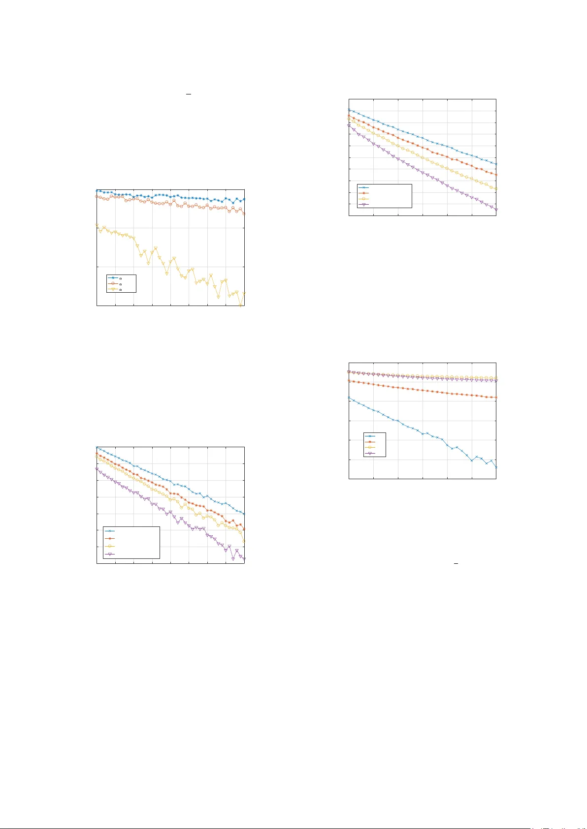
1 Data-Dri v en Nonparametric Existence and Association Problems Y ixian Liu, Y ingbin Liang, Shuguang Cui Abstract —W e in vestigate two closely related nonparametric hypothesis testing problems. In the first problem (i.e., the existence problem), we test whether a testing data stream is generated by one of a set of composite distributions. In the second problem (i.e., the association pr oblem), we test which one of the multiple distributions generates a testing data stream. W e assume that some distributions in the set are unknown with only training sequences generated by the corresponding distributions are a vailable. For both problems, we construct the generalized likelihood (GL) tests, and characterize the error exponents of the maximum error probabilities. For the existence problem, we show that the error exponent is mainly captured by the Chernoff inf ormation between the set of composite distributions and alternative distrib utions. For the association problem, we show that the error exponent is captured by the minimum Chernoff inf ormation between each pair of distributions as well as the KL divergences between the approximated distributions (via training sequences) and the true distributions. W e also show that the ratio between the lengths of training and testing sequences plays an important role in determining the err or decay rate. Index T erms —Multiple hypothesis testing, binary composite hypothesis testing, generalized likelihood test, error exponent, KL divergence I . I N T R O D U C T I O N W E consider two closely related nonparametric hypothe- sis testing problems. W e assume that there are a set of M distinct discrete distributions p 1 , ..., p M , and a training data stream that consists of data samples dra wn from each distribu- tion is av ailable if the corresponding distribution is unknown. Furthermore, a testing data stream is observed, which consists of n samples drawn from an unknown distrib ution. The goal is to solve the following two problems: (1) whether the testing data stream is drawn from one of the M distrib utions; and (2) if the answer is yes, then which distribution generates the testing data stream. Clearly , the first problem tests the existence , i.e., whether the data stream belongs to a set of The work of Y . Liu was supported by University of Chinese Academy of Sciences under UCAS Joint PhD Training Program UCAS[2015]37. The work of Y . Liang was supported in part by D ARP A FunLoL program and by NSF grants ECCS-1609916 and CCF-1617789. The work of S. Cui was supported in part by DoD with grant HDTRA1-13-1-0029, by grant NSFC- 61328102/61629101, and by NSF with grants DMS-1622433, AST -1547436, ECCS-1508051/1659025, and CNS-1343155. Y . Liu is with the Shanghai Institute of Microsystem & Information T echnology , Chinese Academy of Sciences, Shanghai, China and also with the Uni versity of Chinese Academy of Sciences, Beijing, China and also with the School of Information Science & T echnology , ShanghaiT ech University , Shanghai, China (email: liuyx@shanghaitech.edu.cn). Y . Liang is with the Department of Electrical and Computer Engineering, The Ohio State University , Columbus, OH, USA (email: liang.889@osu.edu). S. Cui is with the Department of Electrical and Computer Engineering, Univ ersity of California, Davis, CA, USA (e-mails: sgcu@ucdavis.edu). existent distributions, which is a binary composite hypothesis testing problem. The second problem tests the association , i.e., which distribution the data stream is associated with. For parametric scenarios, where all distributions p 1 , ..., p M are known in advance, both the existence and association prob- lems have been well studied, e.g., [1], [2]. For nonparametric scenarios, where the distributions are unknown, b ut instead, a training data stream generated from each distrib ution is gi ven, previous studies [3]–[5] focused only on the Neyman-Pearson formulation, i.e., giv en the requirement on the error probability for some hypotheses, the error probability for the remaining hypothesis needs to be minimized. The focus of this paper is to solve these problems in the nonparametric case based on a different performance criterion: the maximum of all types of error probabilities. Our focus is on the characterization of the error exponents for such error performance metrics as the sample size enlarges. Our study suggests that such a different performance criterion offers very different understanding and insights about these two problems. The e xistence and association problems naturally corre- spond to two stages of detection problems in many practical applications. For example, in order to detect the operation mode in a cognitive radio (CR) system, a number of CR operation traces are initially collected in the profile, which represent the normal operational patterns of CR systems. Then giv en an observed CR trace, the goal of malware detection is to first determine whether the test CR trace belongs to the existing profile, i.e., whether it is normal or anomalous. If it is anomalous, an alarm of malware infection is triggered. Otherwise, the system needs to determine which existing class the observed operation trace is from, in order to track the operation of the system. The problems considered here can also be used in other applications such as speaker v oice testing [6], [7], signal source and channel detection in wireless networks [8], and homogeneity testing and classification [9], [10]. A. Contributions In this paper , we construct generalized likelihood (GL) tests for the two nonparametric hypothesis testing problems, and characterize the error exponents for the tests. For the existence problem, we show that the error exponent is mainly captured by the Chernoff information between the set of composite distributions and alternative distributions. For the association problem, we show that the error exponent is captured by the minimum Chernoff information between each pair of distribu- tions as well as the KL div ergences between the approximated distributions (via training sequences) and the true distributions. 2 W e also show that the ratio β between the lengths of training and testing sequences plays an important role in determining the error decay behavior . If β → ∞ , i.e., the length of training sequences scales order-wise faster than that of the testing sequence, then the error exponents of the considered nonparametric models conv erge to those of the parametric problems, and hence are optimal. If 0 < β < ∞ , i.e., the lengths of training and testing sequences scale at the same rate, then the GL tests are exponentially consistent (i.e., the error exponents are positi ve). Finally , if β → 0 , i.e., the length of training sequences scales order-wise slower than that of the testing sequence, then the tests are not exponentially consistent. B. Related W ork The multiple hypothesis testing problems have been exten- siv ely studied, e.g., [1] and [2]. For the parametric case, the likelihood ratio test has been studied, and the optimal exponent of the error probability has been characterized in [2]. For the nonparametric case, most studies in the literature, e.g., [3]–[5], focused on the Neyman-Pearson formulation. Our work here on nonparametric hypothesis testing analyzes the exponent of the maximum error probability to quantify the performance. The binary composite hypothesis testing problem has also been studied, e.g., in [11]–[13]. All of these studies focued on the parametric model and adopt the Neyman-Pearson formula- tion. W e study the nonparametric binary composite hypothesis testing in this paper and prov e that the nonparametric test is exponentially consistent in terms of the maximum error probability if the length of training sequences is large enough. Our problem is also related to but dif ferent from the follow- ing models recently studied. One type of anomalous sample detection problems was studied in [14]–[16], in which given a training set of samples generated by one (or more) typical distributions, a new sample needs to be tested whether it is generated from the typical distrib utions or from an anomalous distribution (for example, from a mixture distribution of the typical distribution and another dif ferent distribution). Our model has a sequence of testing samples and our study focuses on characterizing the error exponent, whereas the previous studies did not analyze the error exponent. Furthermore, our existence problem can be viewed as a generalization of the two sample problem, in which two sets of samples respecti vely generated from two unknown distributions are av ailable, and the goal is to test whether the two underlying distributions are identical. Our study is different from the previous studies in [17]–[20] in that our focus is on discrete distrib utions and characterization of the error exponent, whereas previous studies did not characterize the error exponent. Our problem is also related but dif ferent from a class of outlying sequence detection problems studied in [21]–[24]. Our model has training sequences associated with hypotheses, whereas the previous results did not consider such information. The problem on testing closeness of distributions was studied in [25], [26], in which two sets of samples generated from two unknown discrete distributions are av ailable, and the goal is to test whether the two distributions are close in the ℓ 1 norm using as few samples as possible. Our e xistence problem is similar but has composite distributions, and the performance metric of the error exponent is also dif ferent from the pre vious studies. C. Organization The rest of the paper is organized as follows. In Section 2, we describe our problem formulation. In Section 3, we provide our main results on characterization of the error exponents for the two problems. In Section 4, we provide numerical results, and finally in Section 5, we conclude the paper . I I . P R O B L E M F O R M U L A T I O N In this section, we formally define the existence and asso- ciation problems that we study in this paper . Suppose there are in total M distinct discrete distributions p 1 , ..., p M with the support set Y . W e consider a general nonparametric model, in which p i ’ s for 1 6 i 6 M 1 are known, and p i ’ s for M 1 < i 6 M are unknown, where 0 < M 1 6 M . Clearly , if M 1 = M , the problem is fully para- metric with all distributions known. If M 1 = 0 , the problem is fully nonparametric with all distributions unknown. Thus, the model we study here unifies the parametric, semiparametric and nonparametric models; but we refer to such a model as a nonparametric model for simplicity , to which we make our main technical contributions. For each unkno wn distribution p i with i > M 1 , a training sequence t i is a vailable, which consists of ¯ n i.i.d. samples generated by p i . Furthermore, a testing sequence y is observed, which consists of n i.i.d. samples generated by a certain distribution p s ov er the same support Y . W e assume that if p s / ∈ { p 1 , . . . , p M } , then p s is at least a certain distance away from these distributions. More formally , we require that min 1 6 i 6 M C ( p s , p i ) > α, for some α > 0 , (1) where C ( p, q ) is the Chernoff information [2] defined as C ( p, q ) = max λ ∈ [0 , 1] − log    y ∈Y p ( y ) λ q ( y ) 1 − λ   . (2) W e first consider the following two hypotheses: H 0 : p s / ∈ { p 1 , . . . , p M } ; H 1 : p s ∈ { p 1 , . . . , p M } . The goal of our first problem is to determine which hypoth- esis occurs, i.e., whether the testing sequence is generated by one of M existent distributions. W e refer to this problem as the existence pr oblem . Since the hypothesis H 1 contains M sub-hypotheses, the existence problem is a binary composite hypothesis testing problem. W e let δ ( y ) denote a test rule for the existence problem, which maps the testing sequence y to the corresponding hypothesis. Then for the existence problem, we take the following maximum of two types of error probabilities as the performance metric: P e ( δ ) = max { P ( δ = 0 | H 1 ) , P ( δ = 1 | H 0 ) } . (3) 3 W e further define the error exponent of P e ( δ ) as e ( δ ) = lim n →∞ − 1 n log P e ( δ ) . (4) The test δ is consistent if P e ( δ ) con verges to zero as n goes to infinity: lim n →∞ P e ( δ ) = 0 , (5) and the test δ is exponentially consistent if P e ( σ ) con verges to zero exponentially fast with respect to n , i.e., e ( δ ) > 0 . In the existence problem, if the decision is that the testing sequence is generated by one of the existent distributions, then a natural next step is to further identify which distribution generates the testing sequence. W e refer to such a problem as the association pr oblem , which can be formulated as the following multiple hypothesis testing problem: H i : p s = p i , for i = 1 , ..., M , where the goal is to determine which hypothesis occurs. W e let σ ( y ) denote a test rule for the association problem, which maps the testing sequence y to one of the M hypothe- ses. Then, for the association problem, we take the following maximum of M error probabilities as the performance metric: P e ( σ ) = max 1 6 i 6 M P ( σ  = i | H i ) . (6) The error exponent is defined in the same fashion as for the existence problem. I I I . M A I N R E S U LTS In this section, we construct the test rules for the existence and association problems and analyze the performances of these test rules. W e also discuss computational issues of the error exponents. A. Existence Pr oblem: Binary Composite Hypothesis T esting W e first construct a test based on the generalized likelihood. For each kno wn existing distribution, i.e., p i with 1 6 i 6 M 1 , we consider the following likelihood of the testing sequence: P ( y | H i ) = n  k =1 p i ( y k ) = exp {− nH ( γ ( y )) − nD ( γ ( y ) ∥ p i ) } , (7) for 1 6 i 6 M 1 , where γ ( y ) denotes the empirical distrib ution of y giv en by γ ( y ) , number of samples y in y length of y , H ( · ) denotes the entropy given by H ( p ) = −  y ∈Y p ( y ) log p ( y ) , (8) and D ( ·∥· ) denotes the KL div ergence giv en by D ( p ∥ q ) =  y ∈Y p ( y ) log p ( y ) q ( y ) . (9) Since the term H ( γ ( y )) does not depend on the distribution p i , it is dropped from the maximum likelihood test. Hence, the only term that is useful for detection turns out to be D ( γ ( y ) ∥ p i ) , (10) which captures the distance between the empirical distrib ution of the testing sequence and p i . This further suggests that if p i is unknown, i.e., i > M 1 , the corresponding likelihood term should still use the form of (10), but using the empirical distribution γ ( t i ) of p i obtained from the training sequence t i to replace p i in (10), which is hence D ( γ ( y ) ∥ γ ( t i )) . (11) In order to construct a test, it is natural to determine H 0 if the testing sequence is sufficiently far away from all existing distributions, and determine H 1 otherwise. Such a test is given by δ ( y ) : min  min i 6 M 1 D  γ ( y ) ∥ p i  , min i>M 1 D  γ ( y ) ∥ γ ( t i )   H 0 ≷ H 1 α, (12) where α is defined in (1) as the lower bound on the minimum Chernoff information. Note that the left-hand-side of (12) in volv es the KL div er- gence; but the threshold in the right-hand-side corresponds to the Chernof f information. T o e xplain this setup intuitiv ely , we assume that there is only one existing distribution ( M = 1 ), p 0 , in the following argument. With an observed y such that D ( γ ( y ) ∥ p 0 ) > α , there exists an alternative distrib ution d , where C ( p 0 , d ) = α , satisfying D ( γ ( y ) ∥ d ) < α . Hence d can generate y with a larger probability than p 0 and the decision is H 0 . With an observ ed y such that D ( γ ( y ) ∥ p 0 ) < α , we hav e D ( γ ( y ) ∥ d ) > α for any d with C ( p 0 , d ) 6 α . Hence, y is more likely to be generated by p 0 than any alternative distributions and the decision is H 1 . The reader can refer to [2] for more details. In order to understand the nonparametric model, we first analyze the parametric model with M 1 = M . Since all distributions p i ’ s are known, test (12) becomes δ ( y ) : min i D ( γ ( y ) ∥ p i ) H 0 ≷ H 1 α. (13) The performance of such a test is summarized in the following lemma. Lemma 1. T est (13) is exponentially consistent and the exponent of the maximum error pr obability is e = min { e 1 , e 2 } , (14) wher e e 1 is the solution to the following minimization problem: min q,d ∈ ∆ D ( q ∥ d ) (15) s.t. C ( d, p i ) > α , for i 6 M , q ∈ E , with ∆ =  q :  y ∈Y q ( y ) = 1 , 0 6 q ( y ) 6 1  and E = { q : ∃ i s.t. D ( q ∥ p i ) 6 α } , 4 and e 2 is the solution to the following minimization problem: min j 6 M 1 min q ∈ ∆ D ( q ∥ p j ) (16) s.t. q ∈ E , with E being the complementary set of E . Furthermor e, the err or exponent is lower-bounded by α , i.e., e > α . Pr oof. See Appendix B. The above result suggests that the error exponent is lower- bounded by the parameter α , which is the distance between the nearest alternativ e distribution with the set of composite distributions. W e next analyze test (12) for the nonparametric model, in which p i ’ s for i > M 1 are unknown. Clearly , the performance of the test depends on ¯ n n , i.e., the ratio between the lengths of the training and testing sequences. W e let β = lim n →∞ ¯ n n . Then the following theorem summarizes the performance of test (12). Theorem 1. The exponent of the maximum err or pr obability for test (12) is e = min { e 1 , e 2 } , (17) wher e e 1 is the solution to the following minimization problem: min d,q,q M 1 +1 ,...,q M ∈ ∆ D ( q ∥ d ) + β M  k = M 1 +1 D ( q k ∥ p k ) (18) s.t. C ( d, p i ) > α , for i 6 M , ( q , q M 1 +1 , ..., q M ) ∈ E , and e 2 is the solution to the following minimization problem: min i 6 M min q,q M 1 +1 ,...,q M ∈ ∆ D ( q ∥ p i ) + β M  k = M 1 +1 D ( q k ∥ p k ) (19) s.t. ( q , q M 1 +1 , ..., q M ) ∈ E . Her e E =  ( q , q M 1 +1 , ..., q M ) : ∃ i 6 M 1 s.t. D ( q ∥ p i ) 6 α or ∃ i > M 1 s.t. D ( q ∥ q i ) 6 α  , (20) and E is the complementary set of E . If β > 0 , then test (12) is exponentially consistent. If β = ∞ , then the err or exponent is equal to that of the parametric model, and is hence optimal. Pr oof. The proof is provided in Section III-D. The comparison of Lemma 1 and Theorem 1 implies that the error exponent for the nonparametric model is highly affected by the parameter β , which is the ratio between the lengths of training and testing sequences. A larger β results in a better performance. As long as the length of training sequences is not too short compared with the testing sequence such that β > 0 , the test is exponentially consistent. Furthermore, if β = ∞ , i.e., the length of training sequences scales order -wise faster than that of the testing sequence, the error exponent is equal to that of the parametric model. This is reasonable since the hypothesis distributions are well estimated due to the large sample size, so that the performance achiev es that of the parametric case. Corollary 1. If β = 0 and M 1 < M (at least one distribution is unknown), the err or exponent of test (12) is zer o, i.e., the test is not exponentially consistent. Pr oof. Consider the error exponent e 1 giv en in (18). If β = 0 , q M can be set such that C ( q M , p i ) > α , for i 6 M 1 (21) and C ( q M , q i ) > α , for M 1 < i < M . (22) Then let q = q M and d = q M . This setting satisfies the constraint, and thus e 1 = 0 . The condition β = 0 implies that the length of training sequences scales order-wise slower than that of the testing sequence. In such a case, the distributions corresponding to the hypotheses cannot be well estimated, which causes the inconsistency of the test. B. Association Pr oblem: Multiple Hypothesis T esting The problem of the parametric multiple hypothesis testing problem has been well studied in the literature. It has been shown (see [1], [2]) that the following maximum likelihood test achieves the optimal exponent of the maximum error probability: σ ( y ) = arg max i P ( y | H i ) . (23) W e here focus on the nonparametric case. W e construct a generalized maximum likelihood test by replacing each unknown distribution p i (for i > M 1 ) in (23), corresponding to hypothesis i , with the empirical distribution of the training sequence t i . The resulting test is giv en by σ ( y ) = arg max i  P ( y | p i ) , if i 6 M 1 P ( y | γ ( t i )) , if i > M 1  . (24) Applying (7), test (24) is equiv alent to σ ( y ) = arg min i  D ( γ ( y ) ∥ p i ) , if i 6 M 1 D ( γ ( y ) ∥ γ ( t i )) , if i > M 1  . (25) The following theorem characterizes the performance of test (25). Theorem 2. Apply test (25) to the nonpar ametric multiple hy- pothesis testing problem. The err or exponent of the maximum err or pr obability is given by min i,j : i  = j e i,j , wher e e i,j is given as follows. • F or i 6 M 1 and j 6 M 1 , e i,j = C ( p i , p j ) ; • F or i 6 M 1 and j > M 1 , e i,j = min q,q j ∈ ∆ D ( q ∥ p j ) + β D ( q j ∥ p j ) (26) s.t. D ( q ∥ q j ) > D ( q ∥ p i ); 5 • F or i > M 1 and j 6 M 1 , e i,j = min q i ∈ ∆ C ( q i , p j ) + β D ( q i ∥ p i ); (27) • F or i > M 1 and j > M 1 , e i,j = min q,q i ,q j ∈ ∆ D ( q ∥ p j ) + β D ( q i ∥ p i ) + β D ( q j ∥ p j ) (28) s.t. D ( q ∥ q j ) > D ( q ∥ q i ) . Pr oof. The proof is provided in Section III-D. Theorem 2 implies that the error exponent of test (25) is determined by the smallest e i,j , which captures the error exponent for the case where the ground truth is H j but σ ( y ) = i . If both p i and p j are known, e i,j equals the Chernoff information between p i and p j . Thus, if M 1 = M , i.e., all distributions are known, the error exponent reduces to that of the parametric hypothesis testing problem given in [2]. If p i is known, but p j is unknown, (26) consists of two terms: the second term captures the approximation error of the training sequence to p j (where q j can be viewed as the approximation of p j ), and the first term represents the detection error (where q can be viewed as the approximation of the testing distribution). Hence, if q j = p j (i.e., p j is perfectly learned from the training sequence), e i,j becomes C ( p i , p j ) (the parametric case). This also implies that e i,j in such a case is no larger than C ( p i , p j ) . If p i is unknown but p j is known, (27) also consists of two terms: the second term captures the approximation error of the training sequence to p i (where q i can be viewed as the approximation of p i ), and the first term represents the detection error (where q can be viewed as approximation of the testing distrib ution). If neither p i nor p j is known, (28) consists of three terms: the last two terms correspond respectively to the approximation errors of p i and p j , and the first term represents the detection error . In this case, e i,j reduces to C ( p i , p j ) if q i = p i and q j = p j (i.e., the approximations of the distributions are perfect). Thus, the error exponent in this case is no larger than C ( p i , p j ) . The follo wing corollary explains under what conditions the error exponent of test (25) approaches that for parametric hypothesis testing, which serves as an upper bound. Corollary 2. If β > 0 , test (25) is exponentially consis- tent. Especially , if β → ∞ , then the err or exponent goes to min { i,j : i  = j } C ( p i , p j ) , which is optimal, i.e., the error exponent of the nonparametric case appr oaches that of the parametric case if the length of training sequences scales or der-wise faster than that of the testing sequence. Pr oof. Clearly , if β > 0 , the values of (27) is strictly larger than zero. In (26), if q = p j = q j , we have D ( q ∥ q j ) = 0 and D ( q ∥ p i ) > 0 , which contradicts the constraint. The argument is similar for (28). If β → ∞ , then to achie ve the minimum value among (26), (27) and (28), q i and q j must be set as p i and p j . Then it is clear that e i,j in all three cases equals C ( p i , p j ) . Thus, the error exponent of the problem equals min { i,j : i  = j } C ( p i , p j ) . T o further explain the above result, if 0 < β < ∞ , for a larger β , the error between γ ( t i ) and p i is smaller , and hence the exponent of the maximum error probability takes a larger value. The error exponent is strictly larger than zero. In the extreme case with β = ∞ , the error exponent equals that of the fully parametric model, and hence achie ves the optimal v alue. Thus, if the length of training sequences increases much faster than that the testing sequence, the error between γ ( t i ) and p i can be ignored. In such a case, those unknown distributions can be accurately estimated, and hence do not affect the error exponent of the maximum error probability . Corollary 3. If β = 0 and M 1 < M (at least one distribution is unknown), then the err or exponent of the maximum err or pr obability for test (25) equals zer o, i.e., the test is not exponentially consistent. Pr oof. Consider (27). If β = 0 , (27) becomes min q j ∈ ∆ C ( p i , q j ) , which equals zero with q j = p i . Similarly , (28) becomes min q,q i ,q j ∈ ∆ D ( q ∥ p j ) (29) s.t. D ( q ∥ q j ) > D ( q ∥ q i ) , whose optimal value equals zero with q = p j . Since M 1 < M , as least one pair ( i, j ) satisfies i 6 M 1 , j > M 1 , or i > M 1 , j > M 1 . Hence, the error exponent must be zero. The above result implies that if the length of training sequences scales order-wise slower than that of the testing sequence, then the unknown distributions cannot be well estimated, which consequently causes the inconsistency of the test. C. Computation of Err or Exponent It is clear in our analysis that the error exponent in various cases is expressed as the minimum value of an optimization problem, which is noncon ve x and difficult to solve. W e next discuss how to obtain solutions to these optimization problems. First, problem (27) is a min-max problem, which can be written as min max q j ∈ ∆ λ ∈ [0 , 1] F ( q j , λ ) = − log   y ∈Y p j ( y ) λ q i ( y ) 1 − λ  + β  y ∈Y q i ( y ) log q i ( y ) p j ( y ) . (30) It is easy to prov e that the objecti ve function is con vex ov er q j and concav e ov er λ , and for ev ery saddle point ( ˆ q j , ˆ λ ) , we hav e inf sup q j ∈ ∆ λ ∈ [0 , 1] F ( q j , λ ) 6 F ( ˆ q j , ˆ λ ) 6 sup inf λ ∈ [0 , 1] q j ∈ ∆ F ( q j , λ ) . (31) Thus, with the following lemma, all saddle points of prob- lem (30) share the same function value for F ( · , · ) . Lemma 2. (Corollary 37.3.2 in [27]) Let C and D be non- empty closed con vex sets in R m and R n , r espectively , and let 6 K be a continuous finite concave-con vex function on C × D . If either C or D is bounded, we have inf sup v ∈ D u ∈ C K ( u, v ) = sup inf u ∈ C v ∈ D K ( u, v ) . (32) In addition, following from [27], the optimal point of the min-max problem is one of the saddle points of the objective function. Thus, with the discussion above, the problem is solved at a satisfactory le vel as long as we find one saddle point. A sub-gradient method [28] can be utilized to find such a point. Namely , first initialize q (0) j and λ (0) randomly , and then perform sub-gradient decent steps alternatively over q j and λ as q ( k +1) j = P ∆ [ q ( k ) j − s ∇ F q j ( q ( k ) j , λ ( k ) )] (33) λ ( k +1) = P [0 , 1] [ λ ( k ) + s ∇ F λ ( q ( k +1) j , λ ( k ) )] , (34) where s is the step size, P ∆ and P [0 , 1] denote the projections onto the simplex sets ∆ and [0 , 1] , respectiv ely; ∇ F q j and ∇ F λ denote the sub-gradients of F with respect to q j and λ , respectiv ely . Then by choosing an appropriate step size s , the abov e algorithm can be shown to conv erge. The problem in (26) is also a noncon vex problem since the constraint set is nonconv ex. Hence, it is difficult to make the projection onto the constraint set. In this case, we incorporate the constraint set into the objectiv e function as min q,q j ∈ ∆ G ( q , q j ) = D ( q ∥ p j ) + β D ( q j ∥ p j ) + l  D ( q ∥ q j ) − D ( q ∥ p i )  , (35) where l ( x ) =  0 , x > 0 1 2 µx 2 , x < 0 (36) for some µ > 0 . T o minimize the difference between (26) and (35), we need to set a large value for µ . It can be shown that (26) is a Kurdyka-Lojasie wicz (KL) function [29] and Lipschitz continuous near the critical point. Then, we apply the follo wing gradient projection method [29], [30] q ( k +1) j = P ∆ [ q ( k ) j − s ∇ G q j ( q ( k ) , q ( k ) j )] (37) q ( k +1) = P ∆ [ q ( k ) − s ∇ G q ( q ( k ) , q ( k ) j )] , (38) where s is the step size, P ∆ denotes the projection onto the simplex set ∆ , and ∇ G q and ∇ G q j denote the sub-gradients of G with respect to q and q j , respectiv ely . By choosing a q (0) j to be close to p j (e.g., let q (0) j takes the empirical distribution of t j ), and q (0) be in the middle of q (0) j and p i , the iteration can be shown to conv erge to a local minimizer of (35). Problem (28) can be computed similarly as (26), which can be con verted to min q,q i ,q j ∈ ∆ H ( q, q i , q j ) = D ( q ∥ p j ) + β D ( q i ∥ p i ) + β D ( q j ∥ p j ) + l  D ( q ∥ q j ) − D ( q ∥ q i )  . (39) W e then take the gradient projection method as q ( k +1) i = P ∆ [ q ( k ) i − s ∇ H q i ( q ( k ) , q ( k ) i , q ( k ) j )] (40) q ( k +1) j = P ∆ [ q ( k ) j − s ∇ H q j ( q ( k ) , q ( k ) i , q ( k ) j )] (41) q ( k +1) = P ∆ [ q ( k ) − s ∇ H q ( q ( k ) , q ( k ) i , q ( k ) j )] . (42) By choosing a q (0) i near p i , q (0) j near p j , and q (0) in the middle of q (0) j and q (0) i , the iteration con verges to a local minimizer of (39). D. T echnical Pr oofs In this subsection, we pro vide the proofs of Theorems 1 and 2. Pr oof of Theor em 1. Following test (12), the maximum error probability is given by P e ( δ ) = max  P ( δ = 1 | H 0 ) , P ( δ = 0 | H 1 )  . (43) The type I error probability is giv en by P ( δ = 1 | H 0 ) = P  min { min i 6 M 1 D ( γ ( y ) ∥ p i ) , min i>M 1 D ( γ ( y ) ∥ γ ( t i )) } 6 α   H 0  = P  ( γ ( y ) , γ ( t M 1 +1 ) , ..., γ ( t M )) ∈ E   H 0  , where E is defined in (20) and H 0 denotes the hypothesis that y is not generated by one of the M distributions, i.e.,  t k ∼ p k , for k > M 1 ; y ∼ d with C ( d, p i ) > α , for i = 1 , ..., M  . Then the exponent of P ( H 1 | H 0 ) follows from Lemma 3 as the generalization of the Sanov’ s theorem in Appendix A. Similarly , the type II error probability is gi ven by P ( δ = 0 | H 1 ) = max j P  min { min i 6 M 1 D ( γ ( y ) ∥ p i ) , min i>M 1 D ( γ ( y ) ∥ γ ( t i )) } > α   H 1 ,j  = max j P  ( γ ( y ) , γ ( t M 1 +1 ) , ..., γ ( t M )) ∈ E   H 1 ,j  , where E is the complementary set of E and H 1 ,j denotes the hypothesis that y is generated by p j , i.e.,  t k ∼ p k , for k > M 1 ; y ∼ p j  . Then the exponent of P ( H 0 | H 1 ) also follows from Lemma 3 as the generalization of the Sanov’ s theorem in Appendix A. W e next analyze the error exponent. For type I error , the error exponent is e 1 := lim n →∞ 1 n log P ( δ = 1 | H 0 ) . (44) W e compute the v alue of e 1 by Lemma 3 as follows min d,q,q M 1 +1 ,...,q M ∈ ∆ D ( q ∥ d ) + β M  k = M 1 +1 D ( q k ∥ p k ) (45) s.t. C ( d, p i ) > α , for i 6 M , ( q , q M 1 +1 , ..., q M ) ∈ E . Since E in (20) is equal to a union of sets given by E = { ( q , q M 1 +1 , ..., q M ) : D ( q ∥ p 1 ) 6 α } (46) ...... ∪ { ( q , q M 1 +1 , ..., q M ) : D ( q ∥ p M 1 ) 6 α } ∪ { ( q , q M 1 +1 , ..., q M ) : D ( q ∥ q M 1 +1 ) 6 α } ...... ∪ { ( q , q M 1 +1 , ..., q M ) : D ( q ∥ q M ) 6 α } , 7 e 1 equals min j r I ,j , (47) where r I ,j is gi ven as follows. If j > M 1 , then r I ,j is the optimal value of min d,q,q j ∈ ∆ D ( q ∥ d ) + β D ( q j ∥ p j ) (48) s.t. D ( q ∥ q j ) 6 α, C ( d, p i ) > α , for i 6 M . When 0 < β < ∞ , the solution is strictly larger than zero. Otherwise, the objectiv e function equals zero. It means that q = d and q i = p i hold, and then C ( q , q j ) > α , which contradicts D ( q ∥ q j ) 6 α . If β = ∞ and D ( q j ∥ p j ) = 0 , then (48) is equi valent to (49). As a conclusion, the exponent e 1 is strictly larger than zero. If j 6 M 1 , then r I ,j is the optimal value of min d,q ∈ ∆ D ( q ∥ d ) (49) s.t. D ( q ∥ p j ) 6 α, C ( d, p i ) > α , for i 6 M . Problem (49) is similar to (75), which is proved to be no less than α in Appendix B. Thus r I ,j > α for j 6 M 1 . For the type II error , the error exponent is given by e 2 := lim n →∞ 1 n log P ( δ = 0 | H 1 ) . (50) W e compute the value of e 2 by Lemma 3 as follows min i 6 M min q,q M 1 +1 ,...,q M ∈ ∆ D ( q ∥ p i ) + β M  k = M 1 +1 D ( q k ∥ p k ) (51) s.t. ( q , q M 1 +1 , ..., q M ) ∈ E . If 0 < β < ∞ , the optimal value is obviously strictly larger than zero. Otherwise, q = p i and q k = p k for k > M 1 . It contradicts the constraint ( q , q M 1 +1 , ..., q M ) ∈ E . If β = ∞ , D ( q k ∥ p k ) = 0 must hold for ev ery k . Hence, e 2 is the optimal value of min i 6 M min q ∈ ∆ D ( q ∥ p i ) (52) s.t. D ( q ∥ p k ) > α , for k = 1 , ..., M , which is α . Pr oof of Theor em 2. W e first define ¯ p i such that ¯ p i = p i for i 6 M 1 , and ¯ p i = γ ( t i ) for i > M 1 . The maximum error probability is giv en by P e ( σ ) = max i P ( σ  = i | H i ) = max i P {∃ k , D ( γ ( y ) ∥ ¯ p k ) 6 D ( γ ( y ) ∥ ¯ p i ) | H i } . It is easy to see that max j  = i P { D ( γ ( y ) ∥ ¯ p j ) 6 D ( γ ( y ) ∥ ¯ p i ) | H i } 6 P {∃ k , D ( γ ( y ) ∥ ¯ p k ) 6 D ( γ ( y ) ∥ ¯ p i ) | H i } 6  j  = i P { D ( γ ( y ) ∥ ¯ p j ) 6 D ( γ ( y ) ∥ ¯ p i ) | H i } . (53) The exponent of the right-hand-side of (53) can be bounded as lim n →∞ − 1 n log  j  = i P { D ( γ ( y ) ∥ r j ) 6 D ( γ ( y ) ∥ r i ) | H i } ≤ lim n →∞ − 1 n log M max j  = i P { D ( γ ( y ) ∥ r j ) 6 D ( γ ( y ) ∥ r i ) | H i } , = lim n →∞ − 1 n log max j  = i P { D ( γ ( y ) ∥ r j ) 6 D ( γ ( y ) ∥ r i ) | H i } , (54) where the last equality is because M is a fixed constant. Hence, the exponent of the right-hand-side of (53) is equal to that of the left-hand-side of (53). Thus, the error exponent of the maximum error probability is gi ven by E ( σ ) = lim n →∞ − 1 n log P e ( σ ) (55) = lim n →∞ − 1 n log max i P ( σ  = H i | H i ) (56) = min i lim n →∞ − 1 n log max j  = i P { D ( γ ( y ) ∥ ¯ p j ) 6 D ( γ ( y ) ∥ ¯ p i ) | H i } (57) = min i,j : i  = j lim n →∞ − 1 n log P { D ( γ ( y ) ∥ ¯ p j ) 6 D ( γ ( y ) ∥ ¯ p i ) | H i } . (58) Let e i,j := lim n →∞ − 1 n log P { D ( γ ( y ) ∥ ¯ p j ) 6 D ( γ ( y ) ∥ ¯ p i ) | H i } , (59) which represents the exponent of the probability for e vent that y is generated by p i but the GL-test is more likely decide H j than H i . More formally , H i denotes the event  t k ∼ p k , for k > M 1 ; y ∼ p j  . W e next provide the forms for e i,j in four cases. If i 6 M 1 and j 6 M 1 , then ¯ p i = p i and ¯ p j = p j , which are known distributions. Define E = { p : D ( p, p j ) 6 D ( p, p i ) } . Then, follo wing the Sanov’ s theorem in [2], we obtain e i,j = min q ∈ ∆ D ( q ∥ p i ) (60) s.t. D ( q ∥ p j ) 6 D ( q ∥ p i ) = C ( p i , p j ) , where the last equality follows by solving the Lagrangian dual of the optimization problem. If i 6 M 1 and j > M 1 , then ¯ p i = p i which is kno wn; but ¯ p j = γ ( t j ) is the empirical distribution of the training sequence t j . Follo wing from Lemma 3 in Appendix A, we obtain e i,j = min q,q j ∈ ∆ lim n →∞ D ( q ∥ p j ) + β D ( q j ∥ p j ) s.t. D ( q ∥ q j ) > D ( q ∥ p i ) . 8 If i > M 1 and j 6 M 1 , then ¯ p j = p j , which is known; but ¯ p i = γ ( t i ) , which is the empirical distribution of the training sequence. Following from Lemma 3 in Appendix A, we obtain e i,j = min q,q i ∈ ∆ D ( q ∥ p j ) + β D ( q i ∥ p i ) s.t. D ( q ∥ p j ) > D ( q ∥ q i ) = min q i ∈ ∆ β D ( q i ∥ p i ) +  min q D ( q ∥ p j ) s.t. D ( q ∥ p j ) > D ( q ∥ q i ) = min q i ∈ ∆ C ( q i , p j ) + β D ( q i ∥ p i ) , (61) where the last step follows since the inner optimization is the same as (60). If i > M 1 and j > M 1 , then ¯ p i = γ ( t i ) and ¯ p j = γ ( t j ) , both of which are the empirical distributions of the correspond- ing training sequences. Following from the Sanov’ s theorem, we obtain e i,j = min q,q i ,q j ∈ ∆ D ( q ∥ p j ) + β D ( q i ∥ p i ) + β D ( q j ∥ p j ) s.t. D ( q ∥ q j ) > D ( q ∥ q i ) . I V . N U M E R I C A L R E S U LTS In this section, we pro vide numerical results to v alidate the theoretical analyses for both the existence problem and the association problem. 20 25 30 35 40 45 50 55 60 n -0.7 -0.6 -0.5 -0.4 -0.3 -0.2 -0.1 log P e both P 1 P 2 unknown P 1 known, P 2 unknown P 2 known, P 1 unknown both P 1 P 2 known Fig. 1. Existence problem: impact of knowledge of distributions on error decay performance W e first study the existence problem, i.e., the binary com- posite hypothesis testing. For each specific experiment setting, we repeat 5000 random tests for each of the two cases with y respecti vely created by one of the existing distributions or generated by a distribution d , where C ( d, p i ) > α for ev ery p i in the giv en set of composite distributions. In our experiments, d is randomly generated over the support set with probability mass being sampled uniformly from [0 , 1] follo wed by a normalization. Then, bad d ’ s are rejected to make sure C ( d, p i ) > α for every p i . In the the first experiment, we set M = 2 , p 1 = [0 . 1 , 0 . 1 . 0 . 8] , p 2 = [0 . 8 , 0 . 1 , 0 . 1] , α = 0 . 01 , and ¯ n = n , i.e., the length of the training sequences is the same as that of the testing sequence. Fig. 1 plots the changes of log( P e ) with n for four cases with each distributions known or unknown, respectively . It is clear that the parametric case with both distributions known has the best error decay , and the nonparametric case with neither distribution known has the worst error decay . Furthermore, the approximate linearity of the curves implies exponential decay beha viors for all cases, where the slope 1 n log( P e ) of each curve approxi- mates the error exponent. W e then study how the number 20 25 30 35 40 45 50 55 60 n -0.8 -0.7 -0.6 -0.5 -0.4 -0.3 -0.2 -0.1 log P e Only p 1 Only p 1 , p 2 p 1 , p 2 , p 3 Fig. 2. Existence problem: impact of the number of composite distributions on error decay performance of composite distributions affects the performance of the GL test (7). W e consider three distributions: p 1 = [0 . 8 , 0 . 1 , 0 . 1] , p 2 = [0 . 1 , 0 . 1 , 0 . 8] , p 3 = [0 . 6 , 0 . 2 , 0 . 2] , α = 0 . 01 , ¯ n = n , and M 1 = 0 , i.e., all distributions are assumed unknown. W e conduct the experiment for three cases: the set of composite distributions consists of only p 1 , consists of p 1 and p 2 , and consists of all three distributions. Fig. 2 plots the changes of log P e with n for the above cases. It can be seen that the number of composite distributions does not significantly affect the performance in term of the decaying speed. In fact, for the existence problem, the distance between the alternativ e distribution d and the composite set (i.e., the threshold α ) is the major parameter that affects the performance. The number of composite distributions should not affect the performance substantially as long as all composite distributions are far away from the alternative distribution d . 20 25 30 35 40 45 50 55 60 n -0.5 -0.45 -0.4 -0.35 -0.3 -0.25 -0.2 -0.15 -0.1 -0.05 0 log P e =0.1 =0.5 =1 =2 =3 =5 Fig. 3. Existence problem: impact of the length of training sequences on error decay performance 9 W e next study ho w the ratio β = ¯ n n affects the performance. W e set p 1 = [0 . 3 , 0 . 2 , 0 . 5] , p 2 = [0 . 7 , 0 . 2 , 0 . 1] , ¯ n = n , α = 0 . 01 and M 1 = 0 . Fig. 3 plots the changes of log P e with the length n of the sequences for the cases with β = 0 . 1 , 0 . 5 , 1 , 2 , 3 , 5 , respectively . It can be seen that a larger β results in a larger error exponent, which corroborates our theo- rem. W e then study ho w the distance α between the composite 20 25 30 35 40 45 50 55 60 n -1.5 -1 -0.5 0 log P e =0.005 =0.01 =0.05 Fig. 4. Existence problem: impact of the number of composite distributions on error decay performance distributions and the alternativ e distribution affects the test performance. W e set p 1 = [0 . 3 , 0 . 2 , 0 . 5] , p 2 = [0 . 7 , 0 . 2 , 0 . 1] , ¯ n = n , and M 1 = 0 . Fig. 4 plots the changes of log P e with n for the cases with α = 0 . 005 , 0 . 01 , 0 . 05 , respectively . It can be seen that a larger α results a larger error exponent, which corroborates our theorem. In the ne xt se veral experiments, we 20 25 30 35 40 45 50 55 60 n -10 -9 -8 -7 -6 -5 -4 -3 log P e both p 1 p 2 unknown p 1 known, p 2 unknown p 2 known, p 1 unknown both p 1 p 2 known Fig. 5. Association problem: impact of the knowledge of distributions on error decay performance study the association problem, i.e., the multiple hypothesis testing. For each specific experiment setting, we repeat 10000 tests to compute the error probability . W e first study how the knowledge of the distributions affects the error decay performance. W e set the same experiment parameters as that of the first experiment for the existence problem. Fig. 5 plots the performance for the four cases. Similarly as the existence problem, the parametric case has the best error exponent and the nonparametric case has the worst error exponent. W e then study how the number of unknown distrib utions affects the error decay performance of test (25). In this e xper- iment, we set M = 10 , ¯ n = n , and all the 10 distributions are 20 30 40 50 60 70 80 n -2.4 -2.2 -2 -1.8 -1.6 -1.4 -1.2 -1 -0.8 -0.6 -0.4 log P e 0 known distribution 3 known distributions 7 known distributions 10 known distributions Fig. 6. Association problem: impact of the number of unknown distributions on error decay performance created randomly with support size 3 . W e study the cases with M 1 = 0 , 3 , 7 , 10 , respectively . Fig. 6 plots the performance for the four cases. It can be seen that with more distributions known, the error exponent becomes larger , and hence the error decays faster . 20 30 40 50 60 70 80 n -12 -10 -8 -6 -4 -2 0 log P e M=2 M=4 M=6 M=8 Fig. 7. Association problem: impact of the number of distributions (i.e., hypotheses) on error decay performance W e next study how the number of distributions (i.e., hy- potheses) affects the error decay performance. W e study the cases that M = 2 , 4 , 6 , 8 with M 1 = 1 2 M . All distributions are generated randomly with support size 3 and we set ¯ n = n . Fig. 7 plots the performance for all cases, and it can be seen that a larger M yields a worse performance (i.e., smaller error exponent). This is because the error exponent is determined by the smallest distance among all pairs of distributions, and having more distributions may reduce such smallest distance. W e then study ho w the Chernoff information affects the error decay performance. In this experiment, we set M = 2 , M 1 = 0 , ¯ n = n , and study the following three cases. W e set p 1 = [0 . 9 , 0 . 05 , 0 . 05] and p 2 = [0 . 05 , 0 . 05 , 0 . 9] for Case 1, where C ( p 1 , p 2 ) = 0 . 746 ; p 1 = [0 . 8 , 0 . 1 , 0 . 1] and p 2 = [0 . 1 , 0 . 1 , 0 . 8] for Case 2, where C ( p 1 , p 2 ) = 0 . 4069 ; p 1 = [0 . 6 , 0 . 2 , 0 . 2] and p 2 = [0 . 2 , 0 . 2 , 0 . 6] for Case 3, where C ( p 1 , p 2 ) = 0 . 1134 . Fig. 8 plots the performance for all cases, and it can be seen that larger Chernoff distances result in larger error exponents, which corroborates our result. 10 20 25 30 35 40 45 50 55 60 n -12 -11 -10 -9 -8 -7 -6 -5 -4 -3 -2 log P e Large C Middle C Little C Fig. 8. Association problem: impact of the Chernoff information on error decay performance 20 25 30 35 40 45 50 55 60 n -10 -9 -8 -7 -6 -5 -4 -3 -2 -1 log P e Only p 1 , p 2 Only p 1 , p 3 p 1 , p 2 , p 3 Fig. 9. Association problem: impact of the minimum Chernoff information on error decay performance W e ne xt study how the minimum Chernoff information affects the error decay performance. W e consider three dis- tributions: p 1 = [0 . 8 , 0 . 1 , 0 . 1] , p 2 = [0 . 1 , 0 . 1 , 0 . 8] , and p 3 = [0 . 6 , 0 . 2 , 0 . 2] . W e study the following three cases. In Case 1, the hypothesis testing is between p 1 and p 2 , where C ( p 1 , p 2 ) = 0 . 4069 . In Case 2, the hypothesis testing is between p 1 and p 3 , where C ( p 1 , p 3 ) = 0 . 0247 . In Case 3, the hypothesis testing is among p 1 , p 2 and p 3 , where the minimum Chernoff information is given by C ( p 1 , p 3 ) = 0 . 0247 . All distributions are assumed to be unknown and ¯ n = n . Fig. 9 plots the performance for the three cases, and it can be seen that case 1 has the largest error exponent due to its largest minimum Chernof f distance. Furthermore, although case 3 has one more distribution in the hypothesis testing compared to case 2, its error performance is similar to that of case 2 since both cases have the same minimum Chernoff distance. This is in contrast to the existence problem, in which the distance between the composite distributions and the alternati ve distribution determines the performance. W e finally study how the ratio β = ¯ n n affects the error decay performance. W e set p 1 = [0 . 1 , 0 . 1 , 0 . 8] , p 2 = [0 . 8 , 0 . 1 , 0 . 1] , and M 1 = 0 . Fig. 10 plots the error decay performance for the cases respectively with β = 0 . 1 , 0 . 5 , 1 , 2 , 3 , 5 , respectiv ely . It can be seen that a larger β yields a larger error exponent for test (25), which corroborates Corollary 2. 20 25 30 35 40 45 50 55 60 n -12 -11 -10 -9 -8 -7 -6 -5 -4 -3 -2 log P e =0.1 =0.5 =1 =2 =3 =5 Fig. 10. Association problem: impact of the ratio β = ¯ n n of the training and testing sequences on error decay performance V . C O N C L U S I O N In this paper , we have studied the existence and association problems. Our focus has been on the characterization of the error exponent for the maximum error probability . W e have showed that the GL tests are exponentially consistent as long as the number of training samples in each sequence scales no slower than the number of testing samples. As future work, it will be interesting to study the regime where the number of composite distributions in the existence problem or the number of hypotheses in the association problem also goes to infinity , and explore how the number of samples should scale accordingly in order to guarantee the exponential consistency of the GL tests. A P P E N D I X A P RO O F O F A N E X T E N S I O N O F S A N OV ’ S T H E O R E M In this section, we provide an extension of the Sanov’ s Theorem in [2], which is useful for our proofs. Lemma 3. Consider a set P of M + 1 distinct distributions P , P 1 , ..., P M . Suppose t is a sequence with n i.i.d. samples generated by P , and t i is a sequence with ¯ n i.i.d. samples generated by P i , for i = 1 , ..., M , wher e ¯ n is a function of n . Define β = lim n →∞ ¯ n n . Let E ∈ P M +1 be a set of vectors of distributions. Assume E is the closur e of its interior and ¯ n = o ( e n ) . Then we have lim n →∞ − 1 n P  t , t 1 , ..., t M :  γ ( t ) , γ ( t 1 ) , ..., γ ( t M )  ∈ E  = min ( p,p 1 ,...,p M ) ∈ E D ( p ∥ P ) + β ·  i D ( p i ∥ P i ) . (62) Pr oof. The proof follows that of the Sanov’ s theorem in [2]. For a distrib ution P , let T ( P ) denote the set of sequences, the empirical distributions of which are the same as P , i.e., T ( P ) denotes the type of P [2]. 11 W e first deri ve an upper bound: P  t , t 1 , ..., t M :  γ ( t ) , γ ( t 1 ) , ..., γ ( t M )  ∈ E  (63) =  ( p,p 1 ,...,p M ) ∈ E P  T ( p )   i P i  T ( p i )  (64) 6  ( p,p 1 ,...,p M ) ∈ E exp  − nD ( p ∥ P ) −  i ¯ nD ( p i ∥ P i )  (65) 6  ( p,p 1 ,...,p M ) ∈ E max ( p,p 1 ,...,p M ) ∈ E exp  − nD ( p ∥ P ) −  i ¯ nD ( p i ∥ P i )  (66) 6 ( n + M ¯ n + 1) |X | exp  − min ( p,p 1 ,...,p M ) ∈ E  nD ( p ∥ P ) +  i ¯ nD ( p i ∥ P i )   , (67) where |X | is the size of the support set of P . Considering ¯ n = o ( e n ) , we have lim n →∞ 1 n log P  t , t 1 , ..., t M :  γ ( t ) , γ ( t 1 ) , ..., γ ( t M )  ∈ E  6 min ( p,p 1 ,...,p M ) ∈ E D ( p ∥ P ) + β  i D ( p i ∥ P i ) . W e next derive a lower bound. Since E is a close set, we can find a sequence of distributions ( p ( n ) , p ( n ) 1 , ..., p ( n ) M ) such that ( p ( n ) , p ( n ) 1 , ..., p ( n ) M ) ∈ E ∩ P n, ¯ n,..., ¯ n and lim n →∞ D ( p ( n ) ∥ P ) + ¯ n n  i D ( p ( n ) i ∥ P i ) = D ( p ∥ P ) + β  i D ( p i ∥ P i ) , (68) where P n denotes the set of distributions such that the probability of every element is k n for some integer k . Now for any sufficiently large n , we have P  t , t 1 , ..., t m :  γ ( t ) , γ ( t 1 ) , ..., γ ( t M )  ∈ E  =  ( p,p 1 ,...,p M ) ∈ E P  T ( p )   i P i  T ( p i )  > P  T ( p ( n ) )   i P i  T ( p ( n ) i )  > 1  ( n + 1)( ¯ n + 1) M  |X | exp  − nD ( p ( n ) ∥ P ) −  i ¯ nD ( p ( ¯ n ) i ∥ P i )  . (69) Then lim n →∞ − 1 n log P  t , t 1 , ..., t M :  γ ( t ) , γ ( t 1 ) , ..., γ ( t M )  ∈ E  > min ( p,p 1 ,...,p M ) ∈ E D ( p ∥ P ) + β  i D ( p i ∥ P i ) . Combining the upper and lower bounds establishes the lemma. A P P E N D I X B P RO O F O F L E M M A 1 W e separately bound the two terms in the maximum error probability P e = max  P ( δ = 1 | H 0 ) , P ( δ = 0 | H 1 )  . (70) For the test giv en in (12), we deriv e P ( δ = 1 | H 0 ) = P  min i D ( γ ( y ) ∥ p i ) 6 α   H 0  = P  γ ( y ) ∈ E   H 0  , (71) where H 0 denotes the hypothesis that y is not generated by one of the M distributions, i.e.,  y ∼ d with C ( p i , d ) > α , for i = 1 , ..., M  , and the set E is giv en by E = { q : ∃ i s.t. D ( q ∥ p i ) 6 α } . Applying the Sanov’ s theorem, the error exponent of P ( H 1 | H 0 ) is given by e 1 = min d,q ∈ E D ( q ∥ d ) (72) s.t. C ( d, p i ) > α, for i 6 M . W e note that the constraint set E can be further written as the union of m subsets as E = { q : D ( q ∥ p 1 ) 6 α } ∪ { q : D ( q ∥ p 2 ) 6 α } ... ∪ { q : D ( q ∥ p M ) 6 α } . (73) Thus, the optimization problem (72) is equiv alent to finding the optimal solution ov er each subset and then taking the minimum among the solutions as e 1 = min i r i , (74) where r i is the solution of min q D ( q ∥ d ) (75) s.t. D ( q ∥ p i ) 6 α, C ( d, p i ) > α, for i 6 M . W e note that C ( p i , d ) is the optimal v alue of the following optimization problem: min q ′ D ( q ′ ∥ d ) (76) s.t. D ( q ′ ∥ p i ) 6 D ( q ′ ∥ d ) , or equi valently min q ′′ D ( q ′′ ∥ p i ) (77) s.t. D ( q ′′ ∥ p i ) > D ( q ′′ ∥ d ) . W e next prov e by contradiction that if D ( q ∥ p i ) 6 C ( d, p i ) , then D ( q ∥ d ) > C ( d, p i ) for any distributions d and p i ’ s. If D ( q ∥ d ) < C ( d, p i ) , then q does not belong to the constraint set (76). Hence, D ( q ∥ p i ) > D ( q ∥ d ) . As mentioned before, (77) takes the optimal value only when D ( q ′′ ∥ p i ) = D ( q ′′ ∥ d ) . Hence, D ( q ∥ p i ) > D ( q ∥ d ) implies D ( q ∥ p i ) > C ( d, p i ) , 12 which contradicts the assumption. Thus, the original claim is true. Now since C ( d, p i ) > α for all i due to the assumption of the problem, the constraint in (75) implies D ( q ∥ p i ) 6 C ( d, p i ) . Due to the above claim, we conclude that r i > C ( d, p i ) > α for all i . Thus, the error exponent has e 1 > α . W e next deriv e the error exponent e 2 of P ( δ = 0 | H 1 ) and show that it is no less than α . P ( δ = 0 | H 1 ) = max j P  min i D ( γ ( y ) ∥ p i ) > α   H 1 ,j  = max j P  γ ( y ) ∈ E   H 1 ,j  , (78) where H 1 ,j denote the sub-hypothesis that y is generated by p j , i.e., { y ∼ p j } , and E is the complementary set of E giv en by E = { q : min i D ( q ∥ p i ) > α } . (79) Applying Sanov’ s theorem, we obtain the error exponent of P  γ ( y ) ∈ E   H 1 ,j  is e 2 ,j = min q ∈ E D ( q ∥ p j ) , (80) which is clearly no less than α due to the definition of E . Thus, the error exponent of P ( δ = 0 | H 1 ) is min j e 2 ,j , (81) which is also no less than α . A C K N O W L E D G M E N T Y . Liu would like to thank Dr . Zhi Ding for his support of Y ixian Liu’ s visit to Syracuse Uni versity , where this work was performed. R E F E R E N C E S [1] B. C. Levy , Principles of Signal Detection and P arameter Estimation . Springer Science & Business Media, 2008. [2] T . M. Cover and J. A. Thomas, Elements of Information Theory . John W iley & Sons, 2012. [3] J. Ziv , “On classification with empirically observed statistics and uni- versal data compression, ” IEEE T ransactions on Information Theory , vol. 34, no. 2, pp. 278–286, Mar . 1988. [4] M. Gutman, “ Asymptotically optimal classification for multiple tests with empirically observed statistics, ” IEEE T ransactions on Information Theory , vol. 35, no. 2, pp. 401–408, Mar . 1989. [5] O. Zeitouni, J. Ziv , and N. Merhav , “When is the generalized likelihood ratio test optimal?” IEEE T ransactions on Information Theory , vol. 38, no. 5, pp. 1597–1602, Sep. 1992. [6] D. Oshaughnessy , “Speaker recognition, ” IEEE ASSP Magazine , vol. 3, no. 9, pp. 4–17, Oct. 1986. [7] J. P . Campbell, “Speaker recognition: a tutorial, ” Pr oceedings of the IEEE , vol. 85, no. 9, pp. 1437–1462, Sep. 1997. [8] M. Feder and A. Lapidoth, “Universal decoding for channels with memory , ” IEEE Tr ansactions on Information Theory , vol. 44, no. 5, pp. 1726–1745, Sep. 1998. [9] K. Pearson, “On the probability that two independent distributions of frequency are really samples from the same population, ” Biometrika , vol. 8, no. 1/2, pp. 250–254, Jul. 1911. [10] J. Unnikrishnan, “On optimal two sample homogeneity tests for finite alphabets, ” in Pr oc. IEEE International Symposium on Information Theory (ISIT) , Cambridge, MA, USA, Jul. 2012, pp. 2027–2031. [11] E. L. Lehmann and C. Stein, “Most po werful tests of composite hypothe- ses. I. Normal distributions, ” The Annals of Mathematical Statistics , vol. 19, no. 4, pp. 495–516, Dec. 1948. [12] O. Zeitouni, J. Ziv , and N. Merhav , “When is the generalized likelihood ratio test optimal?” IEEE T ransactions on Information Theory , vol. 38, no. 5, pp. 1597–1602, Sep. 1992. [13] Y . W . Huang and P . Moulin, “Strong large deviations for composite hy- pothesis testing, ” in Proc. IEEE International Symposium on Information Theory (ISIT) , Honolulu, HI, USA, Jul. 2014, pp. 556–560. [14] A. O. Hero, “Geometric entropy minimization (GEM) for anomaly detection and localization, ” in Proc. Advances in Neural Information Pr ocessing Systems (NIPS) , V ancouver , BC, Canada, Dec. 2006, pp. 585–592. [15] A. O. Hero and O. Michel, “ Asymptotic theory of greedy approximations to minimal k -point random graphs, ” IEEE T ransactions on Information Theory , vol. 45, no. 6, pp. 1921–1938, Sep. 1999. [16] M. Zhao and V . Saligrama, “ Anomaly detection with score functions based on nearest neighbor graphs, ” in Proc. Advances in Neural Infor- mation Pr ocessing Systems (NIPS) , V ancouver , BC, Canada, Dec. 2009, pp. 2250–2258. [17] P . R. Rosenbaum, “ An exact distribution-free test comparing two multi- variate distributions based on adjacency , ” Journal of the Royal Statistical Society: Series B (Statistical Methodology) , vol. 67, no. 4, pp. 515–530, Aug. 2005. [18] J. H. Friedman and L. C. Rafsky , “Multiv ariate generalizations of the wald-wolfo witz and smirnov two-sample tests, ” The Annals of Statistics , vol. 7, no. 4, pp. 697–717, Jul. [19] P . Hall and N. T ajvidi, “Permutation tests for equality of distributions in high-dimensional settings, ” Biometrika , vol. 89, no. 2, pp. 359–374, Jun. [20] A. Gretton, K. Borgwardt, M. Rasch, B. Sch ¨ olkopf, and A. Smola, “ A kernel two-sample test, ” Journal of Machine Learning Research , vol. 13, pp. 723–773, Mar . 2012. [21] L. Lai, H. V . Poor , Y . Xin, and G. Georgiadis, “Quickest search over multiple sequences, ” IEEE T ransactions on Information Theory , vol. 57, no. 8, pp. 5375–5386, Jul. 2011. [22] Y . Li, S. Nitinawarat, and V . V . V eeravalli, “Univ ersal outlier hypothesis testing, ” IEEE T ransactions on Information Theory , vol. 60, no. 7, pp. 4066–4082, Apr . 2014. [23] S. Zou, Y . Liang, H. V . Poor , and X. Shi, “Nonparametric detection of anomalous data streams, ” IEEE T ransactions on Signal Processing , vol. 65, no. 21, 2017. [24] Y . Bu, S. Zou, and V . V . V eera valli, “Linear complexity exponentially consistent tests for outlying sequence detection, ” in Pr oc. IEEE Inter- national Symposium on Information Theory (ISIT) , Aachen, Germany , Jun. 2017, pp. 988–992. [25] T . Batu, L. Fortnow , R. Rubinfeld, W . D. Smith, and P . White, “T esting closeness of discrete distributions, ” Journal of the A CM , vol. 60, no. 1, pp. 4:1–4:25, Feb . 2013. [26] S.-O. Chan, I. Diakonikolas, G. V aliant, and P . V aliant, “Optimal algorithms for testing closeness of discrete distributions, ” in ACM-SIAM Symposium on Discrete Algorithms (SODA) , Portland, OR, USA, Jan. 2014. [27] R. T . Rockafellar, Conve x Analysis . Princeton Uni versity Press, 2015. [28] A. Nedi ´ c and A. Ozdaglar, “Subgradient methods for saddle-point problems, ” Journal of Optimization Theory and Applications , vol. 142, no. 1, pp. 205–228, Mar . 2009. [29] H. Attouch, J. Bolte, and B. F . Svaiter , “Con vergence of descent methods for semi-algebraic and tame problems: proximal algorithms, forward– backward splitting, and regularized gauss–seidel methods, ” Mathemati- cal Pr ogramming , vol. 137, no. 1-2, pp. 91–129, Aug. 2013. [30] J. C. Dunn, “On the conver gence of projected gradient processes to sin- gular critical points, ” Journal of Optimization Theory and Applications , vol. 55, no. 2, pp. 203–216, Nov . 1987.