Lightweight and Optimized Sound Source Localization and Tracking Methods for Open and Closed Microphone Array Configurations

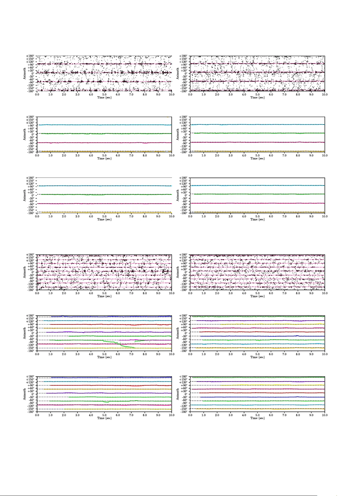
Ligh t w eigh t and Optimized Sound Source Lo calization and T rac king Metho ds for Op en and Closed Microphone Arra y Configurations F rançois Grondin , F rançois Mic haud Dep artment of Ele ctric al Engine ering and Computer Engine ering, Inter disciplinary Institute for T e chnolo gical Innovation (3IT), Université de Sherbr o oke, Sherbr o oke, Québ e c, Canada {fr anc ois.grondin2,fr anc ois.michaud}@usherbr o oke.ca Abstract Human-rob ot interaction in natural settings requires filtering out the different sources of sounds from the environmen t. Suc h ability usually in volv es the use of microphone arrays to lo calize, track and separate sound sources online. Multi- microphone signal processing techniques can improv e robustness to noise but the pro cessing cost increases with the n umber of microphones used, limiting resp onse time and widespread use on different types of mobile rob ots. Since sound source lo calization metho ds are the most expensive in terms of computing resources as they in volv e scanning a large 3D space, minimizing the amount of computations required would facilitate their implemen tation and use on rob ots. The rob ot’s shap e also brings constraints on the microphone array geometry and configurations. In addition, sound source lo calization metho ds usually return noisy features that need to b e smo othed and filtered by tracking the sound sources. This pap er presents a nov el sound source lo calization metho d, called SRP-PHA T-HSD A, that scans space with coarse and fine resolution grids to reduce the n um b er of memory lookups. A microphone directivit y model is used to reduce the n umber of directions to scan and ignore non significant pairs of microphones. A configuration metho d is also introduced to automatically set parameters that are normally empirically tuned according to the shap e of the microphone array . F or sound source trac king, this pap er presents a mo dified 3D Kalman (M3K) metho d capable of simultaneously tracking in 3D the directions of sound sources. Using a 16-microphone array and low cost hardware, results show that SRP-PHA T- HSD A and M3K p erform at least as well as other sound source lo calization and tracking metho ds while using up to 4 and 30 times less computing resources resp ectiv ely . Keywor ds: Sound source lo calization, sound source tracking, microphone array , online pro cessing, em b edded system, mobile rob ot, rob ot audition 1. In tro duction Distan t Sp eec h Recognition (DSR) o ccurs when sp eec h is acquired with one or man y microphone(s) mov ed aw a y from the mouth of the sp eak er, making recognition diffi- cult b ecause of bac kground noise, ov erlapping sp eec h from other sp eak ers, and reverberation [1, 2]. DSR is neces- sary for enabling verbal in teractions without the necessity of using intrusiv e bo dy- or head-moun ted devices. But still, recognizing distant sp eec h robustly remains a c hal- lenge [3]. Microphone arra ys make it p ossible to capture sounds for DSR [2] in h uman-rob ot interaction (HRI). This requires the installation of multiple microphones on the rob ot platform, and pro cess distant sp eec h p erceiv ed b y filtering out noise from fans and actuators on the rob ot and non-stationary background sound sources in reverber- an t environmen ts, fast enough to support live in teractions. This pro cess usually relies first on lo calizing and tracking the p erceiv ed sound sources, to then be able to separate them [4] for sp ecific pro cessing such as sp eec h recognition [5, 6]. Using sound source localization and tracking meth- o ds robust to noise and low computational cost is imp or- tan t [7], as it is usually the first step to engage speech based h uman-rob ot in teraction (HRI). A natural sp eec h HRI re- quires the rob ot to b e able to detect sp eec h commands in noisy en vironments, while av oiding false detections. Figure 1: Block diagram of sound source lo calization and trac king As illustrated by Fig. 1, sound source lo calization (SSL) and sound source trac king (SST) are done in sequence. F or each frame l , SSL uses the captured signals from the M -microphone array X l = { X l 1 , X l 2 , . . . , X l M } and gener- ates V p oten tial sources Ψ l = { ψ l 1 , ψ l 2 , . . . , ψ l V } , where eac h p oten tial source ψ l v consists of a direction of arriv al (DoA) λ l v in Cartesian co ordinates, and the steered b eam- Pr eprint submitte d to R ob otics and Autonomous Systems De c ember 4, 2018 former energy level Λ l v . SSL metho ds provide noisy ob- serv ations of the DoAs of sound sources, caused by the sp oradic activities of sound sources (e.g., the sparsity of sp eec h), combined with the presence of multiple comp et- ing sound sources. SST then uses the p otential sources and returns I track ed sources Φ l = { φ l 1 , φ l 2 , . . . , φ l I } to filter out this noise and pro vide a smooth tra jectory of the sound sources. Improv ed capabilities for SSL and SST can be directly asso ciated with the n umber of microphones used, whic h influences pro cessing requirements [8]. In this process, SSL is the most exp ensive in terms of computation, and a v ariety of SSL algorithms exists. Ras- con et al. [9] present a light weigh t SSL metho d that uses little memory and CPU resources, but is limited to three microphones and scans the DoA of sound source only in 2D. Nesta and Omologo [10] describe a generalized state coherence transform to perform SSL, which is particularly effectiv e when multiple sound sources are present. Ho w- ev er, this metho d relies on indep enden t comp onent anal- ysis (ICA), whic h tak es many seconds to conv erge. Drude et al. [11] use a kernel function that relies on b oth phase and lev el differences, at the cost of increasing the computa- tional load. Lo esch and Y ang [12] also in tro duce a localiza- tion method based on time-frequency sparseness, which re- mains sensitiv e to high reverberation levels. Multiple Sig- nal Classification b ased on Standard Eigenv alue Decompo- sition (SEVD-MUSIC) makes SSL robust to additiv e noise [13]. SEVD-MUSIC, initially used for narrowband signal [14], has b een adapted for broadband sound sources such as sp eech [15], and is robust to noise as long as the latter is less p ow erful than the signals to b e lo calized. Multi- ple Signal Classification based on Generalized Eigenv alue Decomp osition (GEVD-MUSIC) metho d [16] has b een in- tro duced to cop e with this issue, but the latter metho d increases the computations. Multiple Signal Classifica- tion based on Generalized Singular V alue Decomp osition (GSVD-MUSIC) reduces computational load of GEVD- MUSIC and improv es lo calization accuracy [17], but still relies on eigen decomposition of a matrix. Other metho ds tak e adv antage of sp ecific arra y geometries (linear, circular or spherical) to improv e robustness and reduce computa- tional load [18, 19, 20]. Even though in teresting prop erties arise from these geometries, these configurations are less practical for a mobile robot due to physical constraints in- tro duced by its sp ecific shape. SSL can also b e p erformed using a Steered Response Po wer with Phase T ransform (SRP-PHA T). The SRP-PHA T is usually computed using w eighted Generalized Cross-Correlation with Phase T rans- form (GCC-PHA T) at eac h pair of microphones [4, 8]. SRP-PHA T requires less computations than MUSIC-based metho ds, but still requires a significant amoun t of compu- tations when scanning the 3D-space for a large num b er of microphones. Stochastic region con traction [21], hierarc hi- cal search [22, 23, 24] and v ectorization [25] ha v e also been studied to sp eed up scanning with SRP-PHA T, but usu- ally limit the search to a 2D surface and a single source. Marti et al. [26] also prop ose a recursive search o v er coarse and fine grids. This metho d divides space in rectangular v olumes, and maps p oints from the fine grid to only one p oin t on the coarse grid. It how ever neglects microphone directivit y , and also uses an a veraging window ov er the GCC v alues, whic h may reduce the con tribution of a p eak during the coarse scan when neighboring v alues are nega- tiv e. SST metho ds can b e categorized into four types: • Viterbi search. Anguera et al. [27] prop ose a p ost- pro cessing Viterbi method to trac k a sound source o ver time. This metho d introduces a significant la- tency when used online, making it appropriate only for offline pro cessing. T racking is also p erformed on discrete states, whic h restrains the direction of the trac ked source to a fixed grid. • Sequential Mon te Carlo (SMC) filtering. The SMC metho d, also called particle filtering, p erforms lo w la- tency trac king for a single sound source [28, 29, 30]. V alin et al. [4, 8] adapt the SMC metho d to track m ultiple sound sources. This metho d consists in sam- pling the space with finite particles to mo del the non- Gaussian state distribution. SMC allows tracking with con tin uous tra jectories, but requires a significan t amoun t of computations, and is undeterministic be- cause it uses randomly generated particles. • Kalman filtering. Rascon et al. [9] prop ose a ligh tw eigh t method that relies on Kalman filters, whic h allows tracking with contin uous tra jectories and reduce considerably the amoun t of computations. This metho d is how ev er limited to DoAs in spherical co ordinates, using elev ation and azimuth, which gen- erates distortion as the azimuth resolution changes with elev ation. It also introduces azimuth wrapping. Mark ović et al. [31] present an extended Kalman fil- ter on Lie groups (LG-EKF) to p erform directional trac king with an 8-microphone arra y . LG-EKF solv es the azimuth wrapping phenomenon, but limits the trac king to a 2D circle, and is therefore unsuitable for trac king sources on a 3D spherical surface. • Joint probabilistic data asso ciation filter (JPDA). Mark ović et al. [32] introduces this tracking metho d for 3D spherical surface that relies on Ba yesian v on Mises-Fisher estimator. This approach how- ev er requires prior kno wledge of the n um b er of ac- tiv e sources, and neglects the motion mo del for each trac ked source, which leads to switc hed or merged tra- jectories when t wo sources cross each other. T o impro ve SSL and SS T, this pap er introduces a SRP- PHA T metho d referred to as SRP-PHA T-HSDA, for Hier- arc hical Search with Directivity mo del and Automatic cal- ibration, and a tracking metho d based on a mo dified 3D Kalman filter (M3K) using Cartesian coordinates. SRP- PHA T-HSDA scans the 3D space ov er a coarse resolution 2 grid, and then refines search o ver a specific area. It in- cludes a Time Difference of Arriv al (TDOA) uncertaint y mo del to optimize the scan accuracy using v arious grid resolution levels using op en and closed microphone array configurations. A microphone directivity mo del is also used to reduce the num b er of directions to scan and ig- nore non significant pairs of microphones. M3K replaces the SMC filters used in V alin et al. [8] b y Kalman filters, and introduces three new concepts: 1) normalization of the states to restrict the space to a unit sphere; 2) deriv ation of a closed-form expression for the lik elihoo d of a coheren t source to speed up computations; and 3) w eighted update of the Kalman mean vector and cov ariance matrix for si- m ultaneous tracking of sound sources. These mo difications pro vide efficien t trac king of m ultiple sound sources, makes the metho d conv enien t for low-cost em b edded hardware as it requires less computations than the SMC metho d, and solv es the distortion and wrapping introduced b y Kalman filtering with spherical co ordinates. The paper is organized as follo ws. First, Section 2 c har- acterizes the computing requirements of SRP-PHA T in comparison to SEVD-MUSIC, to justify and situate the impro vemen ts brought b y SRP-PHA T-HSDA. Sections 3 and 4 then describe SRP-PHA T-HSD A and M3K, resp ec- tiv ely . Section 5 presen ts the experimental setup in v olv- ing 8 and 16-microphone circular and closed cubic arrays on a mobile rob ot, implementing SSL and SST meth- o ds on a Raspb erry Pi 3. Section 6 presen ts the results obtained from exp eriments comparing SRP-PHA T with SRP-PHA T-HSDA, and M3K with SMC. Finally , Section 7 concludes this pap er with final remarks and future work. 2. Computing Requiremen ts of SRP-PHA T v ersus SEVD-MUSIC SSL is usually divided in tw o tasks: 1) estimation of TDO A, and 2) DoA search o v er the 3D space around the microphone array . The main difference b etw een SRP- PHA T and SEVD-MUSIC lies in T ask 1: SRP-PHA T relies on the Generalized Cross-Correlation with Phase T rans- form metho d (GCC-PHA T), while SEVD-MUSIC uses Singular Eigenv alue Decomp osition (SEVD). The intend here is to demonstrate which metho d is the most efficient for T ask 1, and th en, using this metho d, how can T ask 2 b e further improv ed to reduce computing needs. Both metho ds first capture synchronously the acoustic signals x m from the M microphones in the arra y . These signals are divided in frames of N samples, spaced b y ∆ N samples and m ultiplied by a the sine window w [ n ] : x l m [ n ] = w [ n ] x m [ n + l ∆ N ] (1) with l , i and n representing the frame, microphone and sample indexes, resp ectiv ely . The metho ds then com- pute the Short-Time F ourier T ransform (STFT) with a N - samples real F ast F ourier T ransform (FFT), where the ex- pression X l m [ k ] stands for the sp ectrum at each frequency bin k , and the constant j is the complex num b er √ − 1 : X l m [ k ] = N − 1 X n =0 x l m [ n ] exp ( − j 2 π k n/ N ) (2) The sine window allo ws reconstruction in the time- domain with a 50% frame ov erlap, and thus the same STFT results can b e used for b oth the lo calization and separation steps, which reduces the total amount of com- putations. SRP-PHA T relies on the Generalized Cross- Correlation with Phase T ransform (GCC-PHA T), whic h is computed for each pair of microphones p and q (where p 6 = q ). The Inv erse F ast F ourier T ransform (IFFT) pro- vides an efficien t computation of the GCC-PHA T, giv en that the time dela y n is an integer: r l pq [ n ] = 1 N N − 1 X k =0 X l p [ k ] X l q [ k ] ∗ | X l p [ k ] || X l q [ k ] | +  exp ( j 2 π k n/ N ) (3) The IFFT complexit y dep ends on the num ber of sam- ples per frame N , whic h is usually a pow er of 2. The order of complexity for a real IFFT is O ( N log N ) ). With M ( M − 1) / 2 pairs of microphones, SRP-PHA T computing complexit y reaches O ( M 2 N log N ) . SEVD-MUSIC relies on singular eigenv alue decomp osi- tion of the cross-correlation matrix. The M × M correla- tion matrix R [ k ] is defined as follows, where E { . . . } and { . . . } H stand for the expectation and Hermitian op erators, resp ectiv ely: R [ k ] = E { X [ k ] X [ k ] H } (4) The M × 1 v ector X l [ k ] concatenates the sp ectra of all microphones for each frame l and frequency bin k (where the op erator { . . . } T stands for the transp ose): X l [ k ] =  X l 1 [ k ] X l 2 [ k ] . . . X l M [ k ]  T (5) In practice, the correlation matrix is usually computed at each frame l with an estimator that sums vectors ov er time (a windo w of L frames) for each frequency bin k : R l [ k ] = 1 L L − 1 X ∆ L =0 X l +∆ L [ k ] X l +∆ L [ k ] H (6) SEVD-MUSIC complexit y depends on the size of the matrix R l [ k ] , and is O ( M 3 ) [33]. This op eration is p er- formed at each frequency bin k , for a total of N / 2 bins, whic h leads to an ov erall complexit y of O ( M 3 N ) . T o b etter express the computing requiremen ts of both metho ds, T able 1 presents simulation results of the time (in sec) required to pro cess one frame l , with v arious v al- ues of N and M , on a Raspb erry Pi 3. SRP-PHA T com- pute M ( M − 1) / 2 real N -sample FFT s using the FFTW C library [34], and SVD-MUSIC ev aluates N / 2 SEVD of M × M matrices using the Eigen C++ library [35]. Some metho ds (e.g., [13, 16, 17]) compute SEVD only in the lo wer frequency range (where sp eech is usually observed) 3 to reduce the computational load. How ev er, this discards some useful spectral information in the higher frequen- cies (in speech fricative sounds for instance), which are considered with the SRP-PHA T metho d. T o ensure a fair comparison, both methods treat the whole sp ectral range. F or N = 256 , when the num b er of microphones increase from M = 8 to M = 32 , the pro cessing time in- creases by a factor of 17 . 8 ≈ ( M 1 / M 2 ) 2 = (32 / 8) 2 = 16 for SRP-PHA T, and a factor of 36 . 6 < ( M 1 / M 2 ) 3 = (32 / 8) 3 = 64 for SEVD-MUSIC. The latter factor is less than the exp ected complexity of M 3 , which is probably explained by truncated computation of SVD for small singular v alues. Similarly , for a fixed num ber of micro- phones M = 8 , the complexity increases by a factor of 8 . 9 ≈ ( N 1 / N 2 ) log( N 1 / N 2 ) = (2048 / 256) log(2048 / 256) = 11 for SRP-PHA T, and by a factor of 7 . 3 ≈ ( N 1 / N 2 ) = (2048 / 256) = 8 for SEVD-MUSIC. SRP-PHA T requires from 206 ( M = 8 and N = 2048 ) to 525 ( M = 32 and N = 512 ) less computing time that the SEVD-MUSIC metho d. This suggests that SRP-PHA T is more suitable for online pro cessing, as it p erforms T ask 1 effectiv ely . It is therefore desirable to use SRP-PHA T for T ask 1, and optimize T ask 2 to get an efficient SSL metho d. 3. SRP-PHA T-HSDA Metho d T o understand how SRP-PHA T-HSDA w orks, let us start by explaining SRP-PHA T, to then explain the added particularities of SRP-PHA T-HSDA. Figure 2 illustrates the SRP-PHA T-HSD A metho d, using M microphone sig- nals to lo calize V p oten tial sources. The Microphone Di- rectivit y mo dule and the MSW Automatic Calibration mo dule are used at initialization, and pro vide parame- ters to p erform optimized GCC-PHA T, Maximum Sliding Windo w (MSW) filtering and Hierarchical Search online. Figure 2: Block diagram of SRP-PHA T-HSDA The underlying mec hanism of SRP-PHA T is to search for V p otential sources for each frame l ov er a discrete space [4, 36]. F or eac h potential source, the computed GCC-PHA T frames are filtered using a Maxim um Sliding Windo ws (MSW). The sum of the filtered GCC-PHA T frames for all pairs of microphones provide the acoustic energy for each direction on the discrete space, and the direction with the maximum energy corresp onds to a p o- ten tial source. Once a potential source is obtained, its con tribution is remov ed from the GCC-PHA T frames b y setting the amplitude of the corresponding TDO A to zero, and the space is scanned again. This pro cess is repeated V times until the DoAs ( λ v , v = 1 , . . . , V ) and energy levels ( Λ v , v = 1 , . . . , V ) of all p oten tial sources are generated. A discrete unit sphere pro vides potential DoAs for sound sources. As in [4] and [8], a regular conv ex icosahedron made of 12 p oints defines the initial discrete space, and is refined recursiv ely L times until the desired space resolu- tion is obtained. Figure 3 sho ws the regular icosahedron ( L = 0 ), and subsequent refining iterations levels ( L = 1 and L = 2 ). (a) L = 0 (b) L = 1 (c) L = 2 Figure 3: Discrete unit spheres Eac h p oint on the discrete sphere corresp onds to a unit vector u k , where k stands for the p oint inde x where k = 1 , 2 , . . . , K , and S = { u 1 , u 2 , . . . , u K } is the set that con tains all vectors, where the n umber of p oints K = 10 × 4 L + 2 dep ends on the resolution lev el L . In the SRP-PHA T metho d prop osed in [8], the scan space is refined four times ( L = 4 ) to generate 2562 p oints and obtain a spatial resolution of 3 degrees. T o further reduce SRP-PHA T computations, and main- tain a high lo calization accuracy regardless of the micro- phone array shap e, SRP-PHA T-HSDA adds the follo wing elemen ts: • Micr ophone Dir e ctivity (MD) : When the num ber of microphone M increases, the computational load also increases b y a complexity of O ( M 2 ) . The proposed metho d assumes that microphone ha v e a directivit y pattern, and this introduces constraints that reduces the space to be scanned and the num b er of pairs of mi- crophones to use, which in turn decreases the amoun t of computations. • Maximum Sliding Window Automatic Calibr ation (MSW AC) : TDOA estimation is influenced by the un- certain ty in the sp eed of sound and the microphones p ositions (whic h ma y b e difficult to measure precisely with microphone arra ys of complex geometry), and scan grid discretization, which should be mo delled someho w. The MSW size can b e tuned manually b y hand to maximize lo calization accuracy , but this re- mains a time consum ing task whic h has to be repeated for each new microphone array geometry . The TDO A 4 T able 1: Processing time in sec/frame for {SRP-PHA T, SEVD-MUSIC} and ratio b etw een b oth (between parentheses) M N = 256 N = 512 N = 1024 N = 2048 8 { 1 . 8 E − 4 , 4 . 1 E − 2 } (228) { 3 . 3 E − 4 , 8 . 1 E − 2 } (245) { 7 . 1 E − 4 , 1 . 6 E − 1 } (225) { 1 . 6 E − 3 , 3 . 3 E − 1 } (206) 16 { 7 . 6 E − 4 , 2 . 3 E − 1 } (303) { 1 . 4 E − 3 , 4 . 5 E − 1 } (321) { 3 . 1 E − 3 , 9 . 0 E − 1 } (290) { 6 . 9 E − 3 , 1 . 8 E +0 } (260) 24 { 1 . 8 E − 3 , 7 . 0 E − 1 } (389) { 3 . 3 E − 3 , 1 . 4 E +0 } (424) { 7 . 0 E − 3 , 2 . 8 E +0 } (400) { 1 . 6 E − 2 , 5 . 6 E +0 } (350) 32 { 3 . 2 E − 3 , 1 . 5 E +0 } (469) { 5 . 9 E − 3 , 3 . 1 E +0 } (525) { 1 . 3 E − 2 , 6 . 2 E +0 } (477) { 2 . 9 E − 2 , 1 . 2 E +1 } (524) uncertain ty mo del solves this challenge as it automat- ically tunes the MSW size to maximize lo calization accuracy . • Hier ar chic al Se ar ch (HS) : Searching for p oten tial sources in v olves scanning the 3D space according to a grid with a sp ecific resolution. Finer resolution means b etter precision but higher computation. T o reduce computations, a solution is to first do a scan with a grid at coarse resolution to identify a p otential sound source, and then do another scan with a grid with a fine resolution using the lo cation found during the first scan to pinp oint a more accurate direction. 3.1. Micr ophone Dir e ctivity In a microphone arra y , microphones are usually assumed to be omnidirectional, i.e., acquiring signals with equal gain from all directions. In practice ho w ever, microphones on a robot platform are often mounted on a rigid b o dy , whic h may blo ck the direct propagation path b etw een a sound source and a microphone. The atten uation is mostly due to diffraction, and changes as a function of frequency . Since the exact diffraction mo del is not av ailable, the pro- p osed model relies on simpler assumptions: 1) there is a unit gain for sound sources with a direct propagation path, and 2) the gain is null when the path is blo ck ed by the rob ot b o dy . As the signal to noise ratio is generally unkno wn for the block ed microphones, it is safer to assume a low SNR, and setting the gain to zero preven ts noise to b e injected in the observ ations. Moreo v er, the gain is set constan t for all frequencies, and a smo oth transition band connects the unit and n ull gain regions. This transition band preven ts abrupt changes in gains when the sound source p osition v aries. Figure 4 in tro duces θ ( u , d ) , as de- fined by (7), the angle b etw een a sound source lo cated at u , and the orientation of the microphone mo deled by the unit v ector d . θ ( u , d ) = arccos  u · d | u || d |  (7) Figure 5 illustrates the logistic function that models the gain G ( u , D ) as a function of the angle θ ( u , d ) , giv en in (8). The expression D is a set that con tains the parameters { d , α, β } , where α stands for the angle where the gain is one while β corresponds to the angle at which the gain is n ull. The region b etw een b oth angles can b e viewed as a transition band. Figure 4: Microphone directivit y angle θ as a function of microphone orientation and source direction Figure 5: Microphone gain resp onse G ( u , D ) = 1 1 + exp  20 β − α   θ ( u , d ) − α + β 2  (8) T o mak e SSL more robust to rev erb eration, the scan space is restricted to a sp ecific direction. F or instance, the scan space is limited to the hemisphere that p oints to the ceiling to ignore reflections from the flo or. The unit v ector d 0 stands for the orien tation of the scan space. Since microphone directivity in troduces some con- strain ts on the scan space, the spatial gains G ( u k , D p ) and G ( u k , D q ) need to be large enough for a source lo cated in the direction u k to excite b oth microphones p and q . The gain G ( u k , D 0 ) also needs to b e large enough for this di- rection to be part of the scan space. The mask ζ pq ( u k ) mo dels this condition, where the constan t G min stands for 5 the minimal gain v alue: ζ pq ( u k ) = ( 1 G ( u k , D 0 ) G ( u k , D p ) G ( u k , D q ) ≥ G min 0 otherwise (9) When the mask ζ pq ( u k ) is zero, the v alue of the cor- resp onding sample in the GCC-PHA T frame is negligible and can b e ignored. When all pairs of microphones are uncorrelated ( ζ pq ( u k ) = 0 for all v alues of p and q ), the direction u k can simply b e ignored ( ζ ( u k ) = 0 ): ζ ( u k ) = ( 1 P M p =1 P M q = p +1 ζ pq ( u k ) > 0 0 otherwise (10) Similarly , the GCC-PHA T b etw een microphones p and q needs to b e computed only when ζ pq = 1 , that is when these microphones are excited sim ultaneously at least once for a giv en direction u k : ζ pq = ( 1 P K k =1 ζ pq ( u k ) > 0 0 otherwise (11) 3.2. MSW Automatic Calibr ation The TDO A b etw een t w o microphones m p and m q is giv en b y the expression τ pq ( u ) . Under the far field as- sumption, the TDOA is set according to (12), where u represen ts the normalized direction of the sound source, f S stands for the sample rate (in samples/sec) and c for the sp eed of sound (in m/s). Note that the TDOA is usu- ally given in sec, but is provided in samples here since all pro cessing is p erformed on discrete-time signals. τ pq ( u ) = f S c ( m p − m q ) · u (12) The sp eed of sound v aries according to air temp era- ture, humidit y and pressure. These parameters usually lie within a known range in a ro om (and ev en outside), but it remains difficult to calculate the exact sp eed of sound. In SRP-PHA T-HSDA, the sp eed of sound is mo deled using a random v ariable c ∼ N ( µ c , σ c ) , where µ c is the mean and σ c the standard deviation of the normal distribution. The exact p osition of each microphone is also mo deled by a triv ariate normal distribution m p ∼ N ( µ p , Σ p ) , where µ p stands for the 1 × 3 mean v ector and Σ p for the 3 × 3 co v ariance matrix. The first step consists in solving for the expression a = f S /c (in samples/m). T o make calculations easier, a normally distributed random v ariable η ∼ N (0 , 1) is in- tro duced: a = f S µ c + σ c η (13) The previous equation can b e linearized giv en that µ c  σ c . Expanding this function as a T a ylor series, the follo wing approximation holds: a ≈ f S µ c  1 − σ c µ c η  (14) This results in a b eing a normally distributed random v ariable, with mean µ a and standard deviation σ a . The second step consists in solving the pro jection of the distance b etw een b oth microphones represented by ran- dom v ariables m p and m q , on the deterministic unit v ector u , represen ted b elow as b pq ( u ) : b pq ( u ) = ( m p − m q ) · u (15) The in termediate expression ( m p − m q ) is a random v ariable with a normal distribution ∼ N ( µ pq , Σ pq ) , where µ pq = µ p − µ q and Σ pq = Σ p + Σ q . The p osition un- certain ty is usually significan tly smaller than the distance b et ween b oth microphones, suc h that k µ pq k 2  k Σ pq k , where the expression k . . . k stands for the v ector and ma- trix norms. The random v ariable b pq ( u ) has a normal dis- tribution: b pq ( u ) = µ b,pq ( u ) + σ b,pq ( u ) η = µ pq · u + η q u T Σ pq u (16) The random v ariable τ pq ( u ) is the pro duct of the normal random v ariables a and b pq ( u ) , which gives the follo wing expression: τ pq ( u ) = ( µ a + σ a η a )( µ b,pq ( u ) + σ b,pq ( u ) η b ) (17) where η a and η b are tw o indep endent random v ariables with standard normal distribution. Since µ a  σ a , and µ b,pq ( u )  σ b,pq ( u ) (for all p and q ), the following appro x- imation holds: τ pq ( u ) ≈ µ a µ b,pq ( u ) + µ a σ b,pq ( u ) η b + µ b,pq ( u ) σ a η a (18) The random v ariable τ pq ( u ) therefore exhibits a normal distribution ∼ N ( µ τ ,pq ( u ) , σ τ ,pq ( u )) where: µ τ ,pq ( u ) =  f S µ c  ( µ p − µ q ) · u (19) σ τ ,pq ( u ) = f S µ c s u T ( Σ p + Σ q ) u + [( µ p − µ q ) · u ] 2 σ 2 c µ 2 c (20) This mo dels the TDOA estimation uncertaint y , and is used to configure MSW size. In practice, GCC-PHA T based on FFT generates frames with discrete indexes, and therefore the estimated TDO A v alue (denoted by ˆ τ pq ( u k ) ) for eac h discrete direction u k can be rounded to the closest in teger if no interpolation is p erformed: ˆ τ pq ( u k ) =  f S µ c  ( µ p − µ q ) · u k  (21) T o cop e with the disparity betw een ˆ τ pq ( u k ) and the ob- serv ation of the random v ariable τ pq ( u ) , a MSW filters eac h GCC-PHA T frame for all pairs of microphones, where ˆ r l pq [ n ] stands for the filtered frame. The MSW has a size of 2∆ pq + 1 samples (the frame index l is omitted here for clarit y): ˆ r pq [ n ] = max { r pq [ n − ∆ τ pq ] , . . . , r pq [ n + ∆ τ pq ] } (22) 6 Figure 6: MSW and PDF of the TDOA random v ariable Figure 6 illustrates how the partial area under the prob- abilit y density function (PDF) of τ pq ( u ) stands for the probabilit y the MSW captures the TDOA v alue. The area under the curve corresp onds to the in tegral of the PDF that lies within the in terv al of the MSW, given b y I ( u k ) = [ α ( u k ) , β ( u k )] : α ( u k ) = ˆ τ pq ( u k ) − ∆ τ pq − 0 . 5 (23) β ( u k ) = ˆ τ pq ( u k ) + ∆ τ pq + 0 . 5 (24) P ( τ pq ( u ) ∈ I ( u k )) = Z β ( u k ) α ( u k ) 1 √ 2 π σ 2 exp  − ( τ − µ ) 2 2 σ 2  dτ (25) where µ = µ τ ,pq ( u ) and σ = σ τ ,pq ( u ) . A discrete in tegration ov er space D k is used to estimate the probabilit y P pq that the MSW captures a s ource in a neigh b oring direction to u : P pq ( u ∈ D k ) ≈ E X e =1 P ( τ pq ( v k,e ) ∈ I ( u k )) E (26) An octagon made of E = 4(2 D + 4 D ) + 1 points estimates the discretized surface, where D stands for the num b er of recursiv e iterations. The radius of the octagon corresponds to the distance betw een u k and its closest neigh b or. Figure 7 sho ws o ctagons for D = 0 , 1 and 2 iterations: (a) D = 0 (b) D = 1 (c) D = 2 Figure 7: Discrete octogons F or all directions in the set S = { u 1 , u 2 , . . . , u K } , the probabilit y that the MSW captures sources in neighboring directions is estimated as follows: P pq ( u ∈ D k , 1 ≤ k ≤ K ) ≈ K X k =1 E X e =1 P ( τ pq ( v k,e ) ∈ I ( u k )) K E (27) F or a given discrete direction u k , the probability that the discrete point v k,e is captured for all pairs of micro- phones is estimated with the following expression: P ( v k,e , u k ) ≈ M X p =1 M X q = p +1 P ( τ pq ( v k,e ) ∈ I ( u k )) M ( M − 1) (28) The ob jective is to maximize P ( v k,e , u k ) for all direc- tions u k and discrete p oints v k,e , while keeping the MSW windo w size as small as p ossible to preserve the lo caliza- tion accuracy . T o ac hieve this, Algorithm 1 incremen ts the parameters ∆ τ pq progressiv ely un til the threshold C min is reac hed. This calibration is p erformed once at initializa- tion. Algorithm 1 MSW Automatic Calibration – Offline 1: for all pairs pq do 2: ∆ τ pq ← 0 3: Compute P pq ( u ∈ D k , 1 ≤ k ≤ K ) with (27) 4: end for 5: Compute P ( v k,e , u k ) for all k and e with (28) 6: while min k,e { P ( v k,e , u k ) } < C min do 7: ( pq ) ∗ ← arg min pq { P pq ( u ∈ D k , 1 ≤ k ≤ K ) } 8: ∆ τ ( pq ) ∗ ← ∆ τ ( pq ) ∗ + 1 9: Up date P ( pq ) ∗ ( u ∈ D k , 1 ≤ k ≤ K ) 10: Up date P ( v k,e , u k ) for all k and e 11: end while 3.3. Hier ar chic al Se ar ch Hierarc hical searc h inv olves t wo discrete grids: one with a coarse resolution and the other with a fine resolution. A matc hing matrix M provides a mean to connect at initial- ization the coarse and fine resolution grids, whic h are then used to p erform the hierarchical search. Algorithm 2 first p erforms a scan using the coarse res- olution grid, and then a second scan ov er a region of the fine resolution grid to impro ve accuracy . The expressions ˆ r 0 pq and ˆ r 00 pq stand for the GCC-PHA T frames at pair pq fil- tered b y the MSW for the coarse and fine resolutions grids, resp ectiv ely . T o consider the microphone directivity in the scanning pro cess, the GCC-PHA T result for eac h pair pq and directions u 0 c or u 00 f is summed only when the binary masks ζ pq ( u 0 c ) or ζ pq ( u 00 f ) are set to 1 . The energy levels (defined b y the expressions E 0 and E 00 ) are normalized with the num b er of activ e pairs for each direction (expressed b y T ). The v ariable  is set to a small v alue to a void division b y zero. The coarse scan returns the maximum index c ∗ on the coarse grid, and then the fine scan searc hes all p oin ts f where M ( c ∗ , f ) = 1 . The p oint f ∗ then corresponds to the index of the p oint on the fine grid with the maximum v alue. Scanning for the v potential source returns the DoA λ v = u 00 f ∗ and the corresponding energy lev el Λ v = E 00 ( f ∗ ) . The prop osed Hierarc hical Search inv olv es K 0 + K 00 U /K 0 directions to scan in a verage, compared with K 00 directions 7 for a fixed grid with the same resolution. F or instance, with L 0 = 2 , L 00 = 4 and U = 10 for SRP-PHA T-HSDA, and L = 4 for SRP-PHA T, there are in a verage 320 direc- tions to scan, instead of 2562 . Algorithm 2 Hierarc hical Search Scanning – Online 1: for c = 1 to K 0 do 2: E 0 ( c ) ← 0 , T ← 0 3: for all pairs pq do 4: if ζ pq ( u 0 c ) = 1 then 5: E 0 ( c ) ← E 0 ( c ) + ˆ r 0 pq [ ˆ τ pq ( u 0 c )] 6: T ← T + 1 7: end if 8: end for 9: E 0 ( c ) ← E 0 ( c ) / ( T +  ) 10: end for 11: c ∗ ← arg max c E 0 ( c ) 12: for f = 1 to K 00 do 13: E 00 ( f ) ← 0 , T ← 0 14: if M ( c ∗ , f ) = 1 then 15: for all pairs pq do 16: if ζ pq ( u 00 f ) = 1 then 17: E 00 ( f ) ← E 00 ( f ) + ˆ r 00 pq [ ˆ τ pq ( u 00 f )] 18: T ← T + 1 19: end if 20: end for 21: E 00 ( f ) ← E 00 ( f ) / ( T +  ) 22: end if 23: end for 24: f ∗ ← arg max f E 00 ( f ) 25: return { u 00 f ∗ , E 00 ( f ∗ ) } The matching matrix M that connects the coarse and fine resolution spaces (denoted by S 0 and S 00 , respectively) needs to be generated offline prior to online hierarchical searc h. This K 0 × K 00 matrix, denoted b y the v ariable M , connects each direction from the fine resolution grid (comp osed of K 00 directions) to man y directions in the coarse resolution grid (made of K 0 directions). The similitude betw een a direction u 0 c in S 0 and a direc- tion u 00 f in S 00 is given by δ pq ( c, f ) , which is the length of the in tersection b etw een subsets I 0 pq ( u 0 c ) and I 00 pq ( u 00 f ) : δ pq ( c, f ) =   I 0 pq ( u 0 c ) ∩ I 00 pq ( u 00 f )   (29) where: I 0 pq ( u 0 c ) = [ ˆ τ pq ( u 0 c ) − ∆ τ 0 pq , ˆ τ pq ( u 0 c ) + ∆ τ 0 pq ] (30) I 00 pq ( u 00 f ) = [ ˆ τ pq ( u 00 f ) − ∆ τ 00 pq , ˆ τ pq ( u 00 f ) + ∆ τ 00 pq ] (31) The expressions ∆ τ 0 pq and ∆ τ 00 pq dep end on the window size of the MSW s, computed for the coarse and fine resolu- tions grids, for each pair of microphones pq . Each direction u 00 f in the fine resolution grid is mapped to the U most sim- ilar directions in the coarse resolution grid, derived using Algorithm 3. Algorithm 3 Hierarc hical Search Matching – Offline 1: for f = 1 to K 00 do 2: for c = 1 to K 0 do 3: M ( c, f ) ← 0 4: V ( c ) ← 0 5: for all pairs pq do 6: if ζ pq ( u 0 c ) = 1 and ζ pq ( u 00 f ) = 1 then 7: V ( c ) ← V ( c ) + δ pq ( c, f ) 8: end if 9: end for 10: end for 11: for u = 1 to U do 12: c ∗ ← arg max c V ( c ) 13: M ( c ∗ , f ) ← 1 14: V ( c ∗ ) ← 0 15: end for 16: end for 4. Mo dified 3D Kalman Filters for SST Figure 8 illustrates the nine steps of the M3K metho d, where Normalization (Step B), Likelihoo d (Step D) and Up date (Step H) are introduced to include Kalman filter- ing and replace particle filtering in the m ultiple sources trac king metho d presented by V alin et al. [8]. First, the new states of eac h track ed source are predicted (Step A) and normalized (Step B) in relation to the search space. Second, the p oten tial sources are then assigned (Step C) to either a source curren tly track ed, a new source of a false detection (Steps D, E, F). Third, the metho d then adds (Step G) new sources to b e track ed if needed, and remov es inactiv e sources previously track ed. F ourth, the states of eac h trac k ed source are up dated (Step H) with the relev ant observ ations, and the direction of eac h track ed source is fi- nally estimated (Step I) from the Gaussian distributions. Before presen ting in more details these nine steps in the follo wing subsections, let us first define the Kalman filter mo del used in M3K. A Kalman filter estimates recursively the state of eac h source and pro vides the estimated source direction. Normally distributed random v ariables mo del the 3D-direction ( ( d x ) l i , ( d y ) l i and ( d z ) l i ) and 3D-v elocity ( ( s x ) l i , ( s y ) l i and ( s z ) l i ), where { . . . } T stands the transpose op erator: d l i =  ( d x ) l i ( d y ) l i ( d z ) l i  T (32) s l i =  ( s x ) l i ( s y ) l i ( s z ) l i  T (33) The 6 × 1 random v ector x l i concatenates these p ositions and v elo cities: x l i =  d l i s l i  (34) The Kalman mo del assumes the state evolv es ov er time according to the follo wing linear mo del: x l i = Fx l − 1 i + Bu l i + w i (35) 8 Figure 8: T racking sim ultaneous sound sources using M3K. T rack ed sources are lab eled i = 1 , 2 , 3 and potential sources are labeled v = 1 , 2 , 3 , 4 . where the matrix F stands for the state transition model, B represen ts the control-input matrix, u i l is the con trol v ector and w i mo dels the pro cess noise. In the 6 × 6 matrix F , the expression ∆ T = ∆ N /f S denotes the time interv al (in second) b etw een t wo successiv e frames, with ∆ N b eing the hop size in samples betw een t w o frames, and f S the sample rate in samples p er second: F =          1 0 0 ∆ T 0 0 0 1 0 0 ∆ T 0 0 0 1 0 0 ∆ T 0 0 0 1 0 0 0 0 0 0 1 0 0 0 0 0 0 1          (36) With M3K, there is no control input, and therefore the expression ( Bu i l ) in (35) is ignored. The pro cess noise w i exhibits a multiv ariate normal distribution, where w i ∼ N ( 0 , Q ) . In M3K, the pro cess noise lies in the velocity state and is parametrized with the v ariance σ 2 Q . In this metho d, the parameter σ 2 Q is set to a constan t v alue, but it w ould b e p ossible to hav e it dep end on ∆ T as uncertaint y increases for larger v alues of ∆ T . Q =          0 0 0 0 0 0 0 0 0 0 0 0 0 0 0 0 0 0 0 0 0 σ 2 Q 0 0 0 0 0 0 σ 2 Q 0 0 0 0 0 0 σ 2 Q          (37) The observ ations z i l are represen ted b y random v ariables in the x -, y - and z -directions, obtained from the states: z i l = Hx i l + v (38) where z i l =  ( z x ) l i ( z y ) l i ( z z ) l i  T (39) The 3 × 6 matrix H stands for the observ ation mo del: H =   1 0 0 0 0 0 0 1 0 0 0 0 0 0 1 0 0 0   (40) Expression v ∼ N ( 0 , R ) mo dels the observ ation noise, where the 3 × 3 diagonal cov ariance matrix R is defined as: R =   σ 2 R 0 0 0 σ 2 R 0 0 0 σ 2 R   (41) M3K therefore requires only tw o man ually-tuned param- eters, σ 2 Q and σ 2 R , which influence the tracking sensitivity and inertia of eac h track ed source. 4.1. Pr e diction (Step A) The v ector ˆ x l | l i is the posterior mean of the state, where the 6 × 6 matrix P l | l i stands for the state error p osterior co v ariance matrix of each track ed source i . The trac k- ing metho d predicts new states (also referred to as prior states) for eac h sound source i . Predicted mean v ector and co v ariance matrix are obtained as follo ws: ˆ x l | l − 1 i = F ˆ x l − 1 | l − 1 i (42) P l | l − 1 i = FP l − 1 | l − 1 i F T + Q (43) Eac h prediction step increases the states uncertaint y , whic h is then reduced in the Up date step (Step H) when the trac ked source is asso ciated to a relev ant observ ation. 4.2. Normalization (Step B) The observ ations λ l v stands for sound direction of the p oten tial source v , which constitutes a unit vector. A nor- malization constraint is therefore introduced and generates a new state mean v ector ( ˆ x 0 ) l | l − 1 i , for which the predicted direction ( ˆ d 0 ) l | l − 1 i lies on a unitary sphere and v elo city ( ˆ s 0 ) l | l − 1 i is tangen tial to the sphere surface: ( ˆ x 0 ) l | l − 1 i = " ( ˆ d 0 ) l | l − 1 i ( ˆ s 0 ) l | l − 1 i # (44) where ( ˆ d 0 ) l | l − 1 i = ˆ d l | l − 1 i k ˆ d l | l − 1 i k (45) 9 and ( ˆ s 0 ) l | l − 1 i = ˆ s l | l − 1 i − ˆ d l | l − 1 i ˆ s l | l − 1 i · ˆ d l | l − 1 i k ˆ d l | l − 1 i k 2 ! (46) This manipulation violates the Kalman filter assump- tions, whic h state that all pro cesses are Gaussian and that the system is linear [37]. In practice ho wev er, Kalman filtering remains efficient as this normalization only in- v olves a slight perturbation in direction and v elo cit y , whic h mak es the nonlinearity negligible. During the normalization pro cess, the co v ariance matrix remains unchanged. The Up date step (Step H) ensures that the radial comp onent of the matrix P l | l − 1 i sta ys as small as p ossible such that the PDF (Probability Density F unction) lies mostly on the unit sphere surface. 4.3. Assignment (Step C) Assuming that I sources are track ed, the function f g ( v ) assigns the p otential source at index v to either a false detection ( − 2 ), a new source ( − 1 ), or a previously trac ked source (from 1 to I ): f g ( v ) ∈ {− 2 , − 1 , 1 , 2 , . . . , I } (47) There are V p otential sources that can b e assigned to I + 2 v alues, which leads to G = ( I + 2) V p ossible assign- men ts. The v ector for the assignation g concatenates the V assignment functions for the p oten tial sources: f g =  f g (1) f g (2) . . . f g ( V )  (48) 4.4. Likeliho o d (Step D) The energy lev el Λ l v giv es significan t information regard- ing sound source activit y . When a sound source is active ( A ), which means the source emits a sound, a Gaussian distribution mo dels the energy level and the PDF is given b y: p (Λ l v |A ) = N (Λ l v | µ A , σ A ) (49) where µ A and σ A stand for the mean and standard devia- tion of the normal distribution, resp ectively (for simplicity , w e omit µ A and σ A from the left-hand side of the equa- tion). When the source is inactive, the energy level is mo deled with the same distribution but different parameters: p (Λ l v |I ) = N (Λ l v | µ I , σ I ) (50) where µ I and σ I also represen t the mean and standard de- viation of the normal distribution, resp ectively . Typically the standard deviation σ I is similar to σ A , but the mean µ I is smaller than µ A . Moreov er, the probability that the p oten tial source λ l v is generated b y the track ed source i is obtained with the follo wing volume integral: P ( λ l v |C i ) = Z Z Z p ( λ l v | ( d 0 ) l | l − 1 i ) p (( d 0 ) l | l − 1 i ) dx dy dz (51) The sym b ol C i stands for a coherent source, which de- scrib es a sound source lo cated at a sp ecific direction in space. As mo deled b y the Kalman filter, the probability p (( d 0 ) l | l − 1 i ) follo ws this normal distribution: ( d 0 ) l | l − 1 i ∼ N  µ l i , Σ l i  (52) where µ l i = H ( ˆ x 0 ) l | l − 1 i (53) and Σ l i = HP l | l − 1 i H T (54) Giv en the normalized trac ked source direction ( d 0 ) l | l − 1 i , the following expression represents the PDF when the p o- ten tial source λ l v is observ ed : p ( λ l v | ( d 0 ) l | l − 1 i ) = N  λ l v | ( d 0 ) l | l − 1 i , R  (55) Note that swapping the mean and the random v ariable leads to the same PDF (the expression | . . . | stands for the matrix determinan t): p ( λ l v | ( d 0 ) l | l − 1 i ) = (2 π ) − 3 2 | R | 1 / 2 e − 1 2 ( λ l v − ( d 0 ) l | l − 1 i ) T R − 1 ( λ l v − ( d 0 ) l | l − 1 i ) (56) p (( d 0 ) l | l − 1 i | λ l v ) = (2 π ) − 3 2 | R | 1 / 2 e − 1 2 (( d 0 ) l | l − 1 i − λ l v ) T R − 1 (( d 0 ) l | l − 1 i − λ l i ) (57) The follo wing PDF is therefore defined: p (( d 0 ) i l | l − 1 | λ l v ) = N  ( d 0 ) i l | l − 1 | µ l v , Σ l v  (58) where µ l v = λ l v (59) and Σ l v = R (60) The expression p ( λ l v | ( d 0 ) l | l − 1 i ) is equiv alent to p (( d 0 ) l | l − 1 i | λ l v ) , whic h results in the pro duct of tw o Gaussian distributions. A ccording to [38], this results in a new Gaussian distribution, scaled by the factor ω l iv : p ( λ l v | ( d 0 ) l | l − 1 i ) p (( d 0 ) l | l − 1 i ) = ω l iv N (( d 0 ) l | l − 1 i | µ l iv , Σ l iv ) (61) As derived in [38], the mean vector µ l iv and cov ariance matrix Σ l iv of the resulting distribution are equal to: µ l iv = Σ l iv (( Σ l i ) − 1 µ l i + ( Σ l v ) − 1 µ l v ) (62) Σ l iv = (( Σ l i ) − 1 + ( Σ l v ) − 1 ) − 1 (63) The scaling factor equals to: ω l iv = e ( 1 2 [ ( C 1 ) l iv +( C 2 ) l iv − ( C 3 ) l iv − ( C 4 ) l iv ]) (64) where ( C 1 ) l iv = log | Σ l iv | − log  8 π 3 | Σ l i || Σ l v |  (65) 10 ( C 2 ) l iv = ( µ l iv ) T ( Σ l iv ) − 1 µ l iv (66) ( C 3 ) l iv = ( µ l i ) T ( Σ l i ) − 1 µ l i (67) ( C 4 ) l iv = ( µ l v ) T ( Σ l v ) − 1 µ l v (68) The new Gaussian distribution is substituted in (51), and since the v olume in tegral ov er a triv ariate normal PDF is equal to 1 , the probability is simply equal to the scaling factor computed in (64): P ( λ l v |C i ) = ω l iv Z Z Z N (( d 0 ) l | l − 1 i | µ l iv , Σ l iv ) dx dy dz = ω l iv (69) This provides a direct wa y to compute the probabilit y p ( λ l v |C i ) , which is far more efficient than SMC where the probabilit y is estimated b y sampling the distribution. Fig- ure 9 illustrates the analytic simplification of ho w M3K simplifies the computation of the triple in tegral introduced in (51). Figure 9: Analytic simplification of M3K compared to SMC. The probability that the observ ation λ l v occurs corresp onds to the sum of the pro duct of the probability of eac h state (in blue) with the probability this state generates the observ ation λ l v (in pink). Eac h state probability (in the blue area) is m ultiplied b y the probabilit y that λ l v is observ ed (in pink) by this state. This in v olves a significan t amoun t of computations to sam- ple the state space: this is in fact what the particle filter do es, and wh y the computational load is imp ortant. It is therefore more efficient to compute the closed expression that represents the ov erlap (in green) b etw een state PDF (in blue) and the PDF obtained in (58) from swapping v ariables (in yello w). When a new source app ears or a false detection o ccurs, the observ ation lies anywhere on the scanned space. This is denoted by the symbol D for diffused signal. The SSL mo dule generates DoAs from the scanned space around the microphone array . This space is mo deled b y a unit sphere around the arra y , but the search often partially co vers the complete area due to blind sp ots in tro duced by the microphone array geometry and other constraints. A uniform distribution therefore mo dels the PDF, where ˆ K denotes the num ber of p oints scanned, and K the total n umber of p oints needed to discretize the entire sphere: p ( λ l v |D ) = ˆ K K  1 4 π  = ˆ K 4 π K (70) where 1 / 4 π stands for the uniform distribution o ver a com- plete sphere. The o verall likelihoo d for each p ossible potential-trac k ed source assignation results in the com bination of the energy lev el Λ l v and p otential source p ositions λ l v observ ations, concatenated in the v ector ψ l v . Figure 10 illustrates the three t yp es of assignment: 1. F alse detection: the perceived signal is diffused ( D ) and the source is inactive ( I ). 2. New source: the p erceived signal is diffused ( D ) and the source is activ e ( A ). 3. T rac k ed source i : the p otential source direction is co- heren t with the track ed source i ( C i ) and the source is activ e ( A ). In Fig. 10, it is assumed that the p otential sources are generated only in the top hemisphere, which motiv ates the use of a uniform distribution in this region only for new sources and false detection assignments. Figure 10: T yp es of assignmen ts for each p otential source The probability P ( ψ q l | f g ( q )) is therefore computed as follo ws: P ( ψ l v | f g ( v )) =      P (Λ l v |I ) P ( λ l v |D ) f g ( v ) = − 2 P (Λ l v |A ) P ( λ l v |D ) f g ( v ) = − 1 P (Λ l v |A ) P ( λ l v |C f g ( v ) ) f g ( v ) ≥ 1 (71) Assuming conditional indep endence, the product of the individual probabilities generates the probability for eac h assignmen t: P ( Ψ l | f g ) = V Y v =1 P ( ψ l v | f g ( v )) (72) 4.5. Prior Pr ob abilities (Step E) The prior probabilities that a false detection, a new source or a trac k ed source o ccur are simply defined with the constant parameters P f alse , P new , and P track , resp ec- tiv ely: 11 P ( f g ( v )) =      P f alse f g ( v ) = − 2 P new f g ( v ) = − 1 P track f g ( v ) ≥ 1 (73) These parameters are set empirically but it is observed they hav e little impact on the p erformance of tracking. The prior probabilit y for a given permutation corresp onds to the pro duct of each individual assignment: P ( f g ) = V Y v =1 P ( f g ( v )) (74) 4.6. Posterior Pr ob abilities (Step F) Ba yes’ theorem provides a metho d to obtain the p oste- rior probabilit y for each p ermutation f g : P ( f g | Ψ l ) = P ( Ψ l | f g ) P ( f g ) P G g =1 P ( Ψ l | f g ) P ( f g ) (75) T o calculate the probabilit y that a sp ecific assignment is observ ed, the discrete Kroneck er delta δ [ n ] is introduced: δ [ n ] = ( 0 n 6 = 0 1 n = 0 (76) The probability that the track ed source i generates the p oten tial source v is therefore computed as follo ws: P ( i | ψ l v ) = G X g =1 P ( f g | Ψ l ) δ [ f g ( v ) − i ] (77) The probability that a new source is observed is com- puted similarly: P ( new | ψ l v ) = G X g =1 P ( f g | Ψ l ) δ [ f g ( v ) + 1] (78) Finally , the probabilit y that a trac k ed source is observ ed b y any p otential sources is computed using the com bina- tions where there is an assignmen t b etw een at least one p oten tial source and the track ed source: P ( i | Ψ l ) = G X g =1 P ( f g | Ψ l ) 1 − V Y v =1 (1 − δ [ f g ( v ) − i ]) ! (79) 4.7. A dding and R emoving Sour c es (Step G) Sound sources may app ear and disapp ear dynamically as a new sound source starts or a track ed source stops b eing activ e. When a new source is detected ( p ( new | ψ l v ) > θ new ), this step waits N prob frames to confirm this is really a v alid source and not just a sp oradic detection. During this probation in terv al, the observ ation noise v ariance is set to the parameter ( σ 2 R ) prob to take a small v alue, as it is assumed the observ ations should lie close to each others during this time interv al. The av erage of the probability p ( i | ψ l v ) of the newly track ed sound source is ev aluated, and the source is k ept only if the av erage exceeds the threshold θ prob . Once the existence of a source is confirmed, it is trac k ed un til the source b ecomes inactiv e ( p ( i | Ψ l ) < θ dead ) for at least N dead frames. During this active state, the observ a- tion noise v ariance is increased to the v alue of ( σ 2 R ) activ e , to deal with noisy observ ations and possible motion of the sources. When the source no longer exists, it is deleted and trac king of this source stops. 4.8. Up date (Step H) F or each track ed source, the Kalman gain is computed as follo ws: K l | l − 1 i = P l − 1 | l i H T ( HP l | l − 1 i H T + R ) − 1 (80) The expression ˆ v ( i ) stands for the index of the p otential source that maximizes the probability p ( i | Ψ l ) ): ˆ v ( i ) = arg max v  p ( i | Ψ l )  (81) This pro cess is similar to gating, excepts that the prob- abilit y p ( i | Ψ l ) is used instead of the Mahalanobis distance b et ween the observ ation and the track ed source p osition [39]. The weigh ting factor p ( i | Ψ l ) mo dulates the up date rate of the mean v ector and cov ariance matrix: ˆ x l | l i = ( ˆ x 0 ) l | l − 1 i + p ( i | Ψ l ) K l | l − 1 i ( λ l ˆ v ( i ) − H ( ˆ x 0 ) l | l − 1 i ) (82) P l | l i = P l | l − 1 i − p ( i | Ψ l ) K l | l − 1 i HP l | l − 1 i (83) When no p otential source is clearly asso ciated to the trac ked source i , the probabilit y P ( i | Ψ l ) gets close to zero. The mean of the up dated state ˆ x l | l i is then similar to the mean of the predicted state ˆ x l | l − 1 i . Similarly , the up dated co v ariance matrix P l | l i is similar to the predicted matrix P l | l − 1 i , which grows after each prediction steps. In other w ords, when the observ ations do not provide useful infor- mation, the track ed source mov es according to its inertia while the exact p osition uncertaint y grows. 4.9. Dir e ction Estimation (Step I) The up dated states provide an estimation for eac h sound source direction. This estimated direction φ l i corresp onds to the first moment of the posterior random v ariable ( d 0 ) l | l i : φ l i = Z Z Z N (( d 0 ) l | l i | H ˆ x l | l i , HP l | l i H T )( d 0 ) l | l i dx dy dz (84) whic h simplifies to φ l i = H ˆ x l | l i (85) 12 5. Exp erimen tal Setup Exp erimen ts in v olve tw o 16-microphone arra y configu- rations installed on a mobile rob ot: 1) an op ened micro- phone arra y (OMA) with microphones placed on a circular plane, and 2) a close microphone arra y (CMA) with micro- phones placed on a cubic structure. Figure 11 shows these t wo configurations. The microphones in green are used for exp erimen ts that inv olve only 8 microphones, while b oth green and orange microphones are considered for ex- p erimen ts with 16 microphones. The OMA configuration consists of a circular surface with a diameter of 0 . 254 m, while the CMA configuration in v olves a cubic structure with 0 . 250 m edges, where microphones form many squares with 0 . 145 m edges. With the OMA configuration, all microphones hav e a direct path with the sound sources around the robot, while with the CMA sounds ma y be blo c ked by the cubic structure. (a) OMA (b) CMA Figure 11: 8- and 16-microphone array configurations A diagonal cov ariance matrix mo dels the uncertaint y of microphone p ositions: Σ p =   ( σ xx ) p 0 0 0 ( σ y y ) p 0 0 0 ( σ z z ) p   (86) and is set according to the microphone arra y configuration: • F or OMA, the v ariance ( σ z z ) p in the z -direction is set to zero, while the v ariances ( σ xx ) p and ( σ y y ) p in di- mensions x and y are equal to σ 2 mic . All microphones p oin t to the ceiling, and therefore the direction unit v ector d p is oriented in the p ositive z -axis for all mi- crophones. • F or CMA, all microphones p oint outw ards the cub e, and therefore the direction unit vector d p is oriented in the p ositive or negativ e x and y -axes. The v ari- ances ( σ xx ) p , ( σ y y ) p and ( σ z z ) p are set resp ectively to σ 2 mic if the microphone lies on a face in the plane that spans the corresp onding x -, y - or z -axis, or are set to 0 otherwise. This shape fits in the rob ot perime- ter and leav es ro om for additional sensors on the top of the cub e. All exp eriments are p erformed in a 10 m x 10 m x 5 m ro om. The reverberation level in the ro om (measured b e- t ween 0 Hz and 24000 Hz) reaches RT 60 = 600 msec, and there is no background noise. The rob ot is p ositioned at the cen ter of the ro om. T able 2 lists SRP-PHA T-HSDA parameters used for the exp erimen ts. The frame sizes N corresp ond to a duration of 16 msec ( N /f S ) to match speech stationarity . The hop size ∆ N is se t to provide a 50% ov erlap b etw een frames. The refining lev el is set to D = 1 , which ensures a reliable in tegration and main tains the memory usage and execu- tion time as low as p ossible during initialization. W e set V = 4 to detect up to four simultaneously active sound sources. The parameter σ 2 mic is chosen to mo del the un- certain ty in tro duced b y the mem brane area of all micro- phones. The minimum gain G min gets a v alue close to zero to generate the appropriate masks to limit the searc h space. The mean and standard deviation µ c and σ c are set to model the speed of sound in typical indo or and outdoor conditions. The minimum probability threshold C min is c hosen to ensure a go o d cov erage of the random distribu- tion of the TDO As, while keeping the resolution high. The scan space directivity d 0 p oin ts to the ceiling to remov e reflections from the flo or, whic h corresp onding v alues of α 0 and β 0 to k eep only the top hemisphere. The n umber of links U b et ween the directions in the fine and coarse resolution grids is chosen to ensure an effective mapping while minimizing the num b er of sc anned directions. The resolution levels of the coarse ( L 0 ) and fine ( L 00 ) grids are set to minimize the n umber of lo okups while maintaining a go o d resolution. The parameters α p and β p are c hosen to ensure a smooth directivit y response for all microphones that neglects signals coming from behind the microphones. T able 2: SRP-PHA T-HSDA parameters P arameter V alue P arameter V alue f S (samples/sec) 16000 µ c (m/s) 343 . 0 N (samples) 256 σ c (m/s) 5 . 0 ∆ N (samples) 128 C min 0 . 3 D 1 d 0 [ 0 0 1 ] U 10 L 0 2 V 4 L 00 4 α p ( p > 0) 80 ◦ α 0 80 ◦ β p ( p > 0) 100 ◦ β 0 90 ◦ G min 0 . 1 σ 2 mic 1 E − 6 T able 3 lists the M3K parameters used for the ex- p erimen ts. In these exp eriments, M3K can track up to I max = 10 sources simultaneously . The n umber of track ed sources can exceed the n umber of p otential sources pro- vided b y SSL because the sources are active at different 13 frames. The energy lev el for active and inactiv e sound sources follo ws a Gaussian distribution with means µ A and µ I , and v ariances σ 2 A and σ 2 I . The Ba yesian Extension metho d has b een used to automatically tune these param- eters [40]. How ev er, for these exp eriments, setting these parameters empirically leads to go o d detection rates and trac king accuracy . The parameters ( σ 2 R ) prob and ( σ 2 R ) activ e matc h standard deviations of approximately 3 ◦ and 8 ◦ on the grid, respectively . The expression ( σ 2 R ) prob is smaller than ( σ 2 R ) activ e since the observ ations lie close to eac h other during the short probation interv al. The v ariance of the pro cess noise σ 2 Q is set to a v alue high enough to follo w a source that c hanges direction, but low enough to preserve the source inertia. Parameters P f alse , P new and P track are c hosen empirically: they hav e little impact on trac king p erformance as long as P track is greater than P f alse and P new . New source detection requires θ new to b e close to a probability of 1 , but small enough to detect new sources, and is therefore set empirically to 0 . 7 . Probation corresp onds to the time interv al while a source is track ed but not displa y ed. It is defined as N prob ∆ N /f S sec, whic h lies within the duration range of a single phoneme (i.e., 40 msec) [41]. The num b er of inactiv e frames N dead ∆ N /f S is set to matc h a duration of 1.2 sec, whic h is a reasonable silence p erio d to consider a source is no longer active. T able 3: SST Module Parameters P arameters V alues P arameters V alues I max 10 P f alse 0 . 1 µ A 0 . 20 P new 0 . 1 σ 2 A 0 . 0025 P track 0 . 8 µ I 0 . 10 θ new 0.7 σ 2 I 0 . 0025 N prob 5 ( σ 2 R ) prob 0 . 0015 θ prob 0.8 ( σ 2 R ) activ e 0 . 0030 N dead 150 σ 2 Q 0 . 000009 θ dead 0 . 9 6. Results In this section results are presented for SSL by compar- ing SRP-PHA T-HSD A with SRP-PHA T, and for SST by comparing M3K with SMC and using SRP-PHA T-HSDA. 6.1. Sound Sour c e L o c alization Lo calization accuracy is computed with the prop osed metho d to v alidate the MSW Automatic Calibration metho d. The C PU usage for a single core b etw een SRP- PHA T and the proposed SRP-PHA T-HSDA is measured to compare computational load on a Raspb erry Pi 3 (equipp ed with a ARM Cortex-A53 Quad-Core pro cessor clo c ked at 1.2 GHz). P erformance with multiple sp eech sources around the rob ot is also ev aluated. Both metho ds are implemented with the ODAS framew ork (Open em bed- deD Audition System) in C language (without Neon/SSE optimization), whic h is av ailable online as op en source 1 . 6.1.1. L o c alization A c cur acy T o ev aluate lo calization accuracy , the rob ot is installed in the middle of a large ro om and a loudspeaker is p osi- tioned r = 3 m a wa y at an height of h = 1 . 15 m referenced to origin of the microphone array , at azimuths of φ = 0 ◦ , 10 ◦ , . . . , 350 ◦ , for a total of 36 p ositions. F or eac h p o- sition, a white noise signal plays in the loudsp eaker for 2 sec. The recorded signals are then mixed to generate t wo activ e sources at differen t azim uths φ 1 and φ 2 , as sho wn in Fig. 12. All p ermutations of { φ 1 , φ 2 } , where φ 1 6 = φ 2 , Figure 12: Setup for SSL ( { 0 ◦ , 10 ◦ } , { 0 ◦ , 20 ◦ } , . . . , { 350 ◦ , 340 ◦ } ) are in vestigated, for a total of 1260 p ermutations. The expression γ ( φ ) stands for the DoA in Cartesian co ordin ates that corre- sp onds to azimuth φ : γ ( φ ) = 1 √ r 2 + h 2  r cos( φ ) r sin( φ ) h  (87) The Root Mean Square Error (RMSE) corresp onds to the smallest distance b etw een p otential source v and b oth theoretical DoAs at angles φ 1 and φ 2 : RMSE v = min {k λ v − γ ( φ 1 ) k , k λ v − γ ( φ 2 ) k} (88) The av erage RMSE for b oth p otential sources v = 1 and v = 2 provide insight regarding lo calization accuracy: RMSE = RMSE 1 + RMSE 2 2 (89) T able 4 present the RMSE results with 16 microphones, resp ectiv ely . The SRP-PHA T metho d for a single grid with refining level L = 1 , 2 , 3 , 4 and omni-directional mi- crophone mo del p erforms localization with fixed v alu es for the size of MSW ( ∆ τ pq = 0 , 1 , 2 , 3 ), and is compared with the SRP-PHA T-HSD A metho d which automatically calibrates ∆ τ pq (MSW A C) and uses the microphone di- rectivit y mo del. Moreov er, Hierarchical Searc h using t wo grids with differen t refining lev els L = { 2 , 4 } (which means L 0 = 2 and L 00 = 4 ) is also examined, for fixed and au- tomatically selected v alues of ∆ τ pq . The RMSE v alues in b old stand for the smallest v alues across ∆ τ pq = 0 , 1 , 2 , 3 and MSW A C, for a given refining level. 1 http:/odas.io 14 T able 4: SSL RMSE with tw o active sound sources and 16 microphones Configuration ∆ τ pq Microphone Directivit y L 1 2 3 4 { 2 , 4 } OMA 0 Omni-directional 0 . 279 0 . 140 0 . 081 0 . 064 0 . 064 1 Omni-directional 0 . 231 0 . 186 0 . 208 0 . 222 0 . 222 2 Omni-directional 0 . 311 0 . 349 0 . 375 0 . 384 0 . 385 3 Omni-directional 0 . 501 0 . 559 0 . 584 0 . 596 0 . 596 MSW A C Directive 0 . 232 0 . 148 0 . 080 0 . 063 0 . 064 CMA 0 Omni-directional 0 . 528 0 . 282 0 . 153 0 . 128 0 . 165 1 Omni-directional 0 . 414 0 . 286 0 . 272 0 . 273 0 . 285 2 Omni-directional 0 . 477 0 . 448 0 . 454 0 . 456 0 . 454 3 Omni-directional 0 . 599 0 . 624 0 . 649 0 . 657 0 . 649 MSW A C Directive 0 . 300 0 . 195 0 . 117 0 . 094 0 . 103 Results suggest that when set to a constan t, the ideal v alue of ∆ τ pq c hanges according to the grid resolution lev el L . F or the OMA configuration, setting automatically the v alue of ∆ τ pq leads to the same accuracy as when the b est constan t v alue of ∆ τ pq is c hosen except for the case when L = 1 and L = 2 , where the RMSE is slightly higher, yet almost equal. This o ccurs when the size of the MSW is o verestimated. F or the CMA configuration, the automatic calibration com bined with the directivit y model leads to b etter accuracy compared to constan t v alues chosen em- pirically and the omni-directional mo del. Finally , Hierar- c hical Search ( L = { 2 , 4 } ) provides the same accuracy as the high resolution ( L = 4 ) grid with OMA, and increases the RMSE marginally with CMA. It is p ossible to impro ve the accuracy of Hierarc hical Search such that it matches the fixed grid with L = 4 b y increasing the parameters U , at the cost of increasing slightly the computational load. 6.1.2. Computational L o ad Figure 13 shows the CPU usage for a single core on the Raspb erry Pi 3. Results demonstrate that SRP-PHA T- HSD A reduces considerably computational load. CPU us- age reduces by a factor of four for the CMA configura- tion with 16 microphones. The SRP-PHA T-HSDA uses less computations with CMA than OMA, which is due to the microphone directivity mo del that disregards the non significan t pairs of microphones. SRP-PHA T-HSD A is ca- pable of online p erformance with 16 microphones, while SRP-PHA T can not b e processed online past 12 micro- phones, as the CPU usage exceeds 100% (106% and 105% with 13 microphones for CMA and OMA, resp ectively). 6.1.3. L o c alization of Multiple Sp e e ch Sour c es Fiv e sp eech sources are play ed in loudsp eakers lo cated at azimuths φ 1 = 0 ◦ , φ 2 = 60 ◦ , φ 3 = 120 ◦ , φ 4 = 200 ◦ and φ 5 = 270 ◦ . Sources 1 , 3 and 5 are male sp eakers while sources 2 and 4 are female sp eakers. They all sp eak con- tin uously during 10 seconds. Since potential sources are Figure 13: CPU Usage on a single core on a Raspberry Pi 3 significan t when the energy level Λ v is high, only the most energetic p otential sources (25% of all potential sources whic h ha ve the highest v alues of Λ v ) are plotted in Fig. 14 and Fig. 15, for the OMA configuration with 8 and 16 microphones, resp ectively , and in Fig. 16 and Fig. 17, for the CMA configuration with 8 and 16 microphones, resp ectiv ely . Results show that for the OMA configuration, b oth SRP-PHA T and SRP-PHA T-HSDA p erform similarly: with b oth metho ds, there are few false detections. The HSD A metho d therefore p erforms similarly with the stan- dard PHA T for OMA configurations, but requires less computations. On the other hand, the SRP-PHA T-HSDA outp erforms the SRP-PHA T metho d with the CMA con- figuration: there are numerous false detections with SRP- PHA T for 8 microphones, while there are fewer with SRP- PHA T-HSDA, and there are many false detections with SRP-PHA T with 16 microphones, while there is only one at 5 sec with the prop osed SRP-PHA T-HSD A. This ro- bustness is due to the Microphone Directivity mo del that exploits the direct path of sound propagation with closed microphone arra y shapes. This suggests that the HSD A 15 (a) SRP-PHA T (b) SRP-PHA T-HSDA Figure 14: Azimuths obtained with the OMA configuration for five speech sources and 8 microphones (true azim uths are plotted in blue, and false detections are in red) (a) SRP-PHA T (b) SRP-PHA T-HSDA Figure 15: Azimuths obtained with the OMA configuration for five speech sources and 16 microphones (true azimuths are plotted in blue, and false detections are in red) (a) SRP-PHA T (b) SRP-PHA T-HSDA Figure 16: Azimuths obtained with the CMA configuration for fiv e speech sources and 8 microphones (true azim uths are plotted in blue, and false detections are in red) metho d should b e used with CMA configurations to reduce false detections. (a) SRP-PHA T (b) SRP-PHA T-HSDA Figure 17: Azimuths obtained with the CMA configuration for fiv e speech sources and 16 microphones (true azimuths are plotted in blue, and false detections are in red) 6.2. Sound Sour c e T r acking The prop osed M3K metho d is tested in a real en vi- ronmen t on a mobile rob ot and compared with the SMC metho d. The computational load of M3K is first mea- sured on a low-cost embedded hardware, and compared to the load with SMC. T rac king exp erimen ts with static and mo ving sound sources are then examined. Male and fe- male speakers talking in English are used as sound sources. Only the tracking of the azimut is presented, b ecause for b oth metho ds elev ation matc hed the height of the sound sources for all trials. 6.2.1. Computational L o ad A Raspberry Pi 3 is used to compare CPU usage of M3K and SMC for a single core with C co de, whic h is not optimized with Neon/SSE instructions. T o assess the per- formance in terms of the num b er of trac ked sources, the maxim um num b er of simultaneously trac ked sources I max is set from 1 to 10 , while there are 10 active sound sources lo cated at the follo wing azim uths: 0 ◦ , 40 ◦ , 70 ◦ , 100 ◦ , 140 ◦ , 180 ◦ , 220 ◦ , 260 ◦ , 300 ◦ and 330 ◦ . Figure 18 sho ws the CPU usage with b oth metho ds. The SMC method allows on- line pro cessing for up to four track ed sources, and then CPU usage exceeds 100% (the usage increases to 127% with fiv e trac ked sources). The M3K reduces significan tly the amoun t of computations, pro viding online pro cessing with eigh t track ed sources (the usage is slightly ab ov e 100% with nine track ed sources). When a single source is track ed, M3K uses 0 . 8% of the CPU (rounded to 1% on Fig. 18), while SMC reaches a CPU usage of 24% . The M3K metho d is therefore up to 30 times more effective in terms of computational load. As the num ber of trac ked sources increases, the n umber of assignments ( I + 2) V rises exp onen tially , which explains the high CPU usage for large v alues of I . 6.2.2. Static Sound Sour c es The first expriment conducted inv olves four static sources, to repro duce the test conditions of [8]. In this 16 Figure 18: CPU Usage of SMC and M3K on a Raspberry Pi 3 exp erimen t, a loudspeaker is p ositioned r = 3 m a wa y from the rob ot, at azimuths of 10 ◦ , 100 ◦ , 190 ◦ , and 280 ◦ , and a heigh t of 1 . 2 m related to the rob ot microphone arra y origin, as shown in Fig. 19. Figure 20 sho ws the p o- Figure 19: Setup for SST ten tial sources generated b y SRP-PHA T-HSD A and the corresp onding track ed sources using SMC and M3K for the OMA and CMA configurations. T rack ed sources tra- jectories illustrate that M3K p erforms as well as SMC for b oth OMA and CMA configurations. W e then increased the n umber of track ed sound sources to nine, reaching the limit of acceptable trac king perfor- mance. These nine static sp eech sources, at azim uths of 10 ◦ , 50 ◦ , 90 ◦ , 130 ◦ , 170 ◦ , 210 ◦ , 250 ◦ , 290 ◦ and 330 ◦ . Fig- ure 21 shows the p otential sources and the tracking results. The high n umber of sources makes detection and trac king more challenging for tw o reasons: 1) sources are closer to eac h other, which mak es differen tiation difficult betw een t wo static sources; and 2) observ ations sparsity increases, whic h means eac h sound source gets assigned fewer p oten- tial sources from the SSL mo dule as they are distributed o ver all active sources. SMC p erforms tracking accurately with the CMA configuration, but there is an error in track- ing with the OMA that starts at 5 sec. The source drifts, and another source is created to trac k the source at 290 ◦ . M3K, whic h assumes all sources hav e a n ull or constan t v e- lo cit y , mo dels more accurately the static sound source dy- namics with b oth configurations. With nine sources, b oth M3K and SMC also take more time to detect all sources (up to 1 sec of latency) due to observ ations sparsity . 6.2.3. Moving Sound Sour c es T wo tests conditions are examined. The first in volv es four moving sources crossing, tested with OMA and CMA. F or this exp eriment, a male speaker p erforms four tra jecto- ries at r = 3 m aw a y from the robot, starting from different p ositions as illustrated by Fig. 22a. These recordings are com bined to generate the case of four sim ultaneous mo ving sources that cross each other. The second test condition in volv es mo ving sound sources follo wing each other. A male sp eaker p erformed four tra jectories at r = 3 m aw a y from the rob ot, whic h are mixed together such that sources are follo wing each other, as shown in Fig. 22b. Figure 23 presents trac king results using b oth methods, with the OMA and CMA configurations. Results demon- strate that M3K performs as well as SMC with OMA, and M3K p erforms b etter than SMC with CMA. In fact, sources crossing at 5 sec are p ermuted with SMC, while they keep their resp ectiv e tra jectories with M3K. This is caused b y the mo del dynamics that pro vides more inertia with M3K than with SMC. There is also a false detection at 6 sec, with the same azimuth and a differen t elev ation, whic h is due to reverberation from the flo or. Figure 24 shows the p otential sources and trac king re- sults with the OMA and CMA configurations. With OMA, b oth tracking metho ds p erform w ell, except when one source b ecomes inactive around 6 sec: M3K remov es the source in Fig. 24e as required, but SMC k eeps tracking it and even tually div erges in the wrong direction, as the particle filter with the parameters prop osed in [8] is more sensitiv e to noisy observ ations. Similarly , with CMA, M3K and SMC track the sources accurately , except that both k eep tracking the source that b ecomes inactiv e around 7 sec. T o remov e inactive source quickly , the parameter µ A defined in T able 3 could be increased, at the cost of de- tecting new sources with more latency . 7. Conclusion This pap er introduces nov el SSL and SST metho ds de- signed to impro v e robustness to noise by allo wing to in- crease the num ber of microphones used while reducing computational load. F or SSL, SRP-PHA T-HSD A scans the 3D space more efficiently using t wo grids of coarse and fine resolution. A microphone directivity mo del also reduces the amount of computations and reduces false de- tections with Closed Microphone Arra y (CMA) configura- tions. The TDOA uncertaint y mo del optimizes the MSW sizes according to the array geometry and the uncertain- ties in the sp eed of sound and the p ositions of the micro- phones. M3K provides efficient tracking of sound sources in v arious conditions (simultaneous static sources, sim ul- taneous moving sources crossing and sim ultaneous mo ving sources follo wing eac h other), with accuracy comparable or b etter compared to SMC, and reduces by up to 30 times the amoun t of computations. This efficiency mak es the metho d more appropriate for implementing SST on low- cost em b edded hardware. In future w ork, the SRP-PHA T-HSD A metho d could in- clude a mo del that optimizes the Maximum Sliding Win- do w size for each individual p oint to scan and pair of mi- crophones (instead of only eac h pair of microphones as it is currently the case). M3K relies on a single dynamic 17 (a) Potential sources (OMA) (b) Potential sources (CMA) (c) T racked sources with SMC (OMA) (d) T racked sources with SMC (CMA) (e) T racked sources with M3K (OMA) (f ) T rac ked sources with M3K (CMA) Figure 20: Azim uths of four static speech sources (a) Potential sources (OMA) (b) Potential sources (CMA) (c) T racked sources with SMC (OMA) (d) T racked sources with SMC (CMA) (e) T racked sources with M3K (OMA) (f ) T rac ked sources with M3K (CMA) Figure 21: Azim uths of nine static sources 18 (a) Crossing sources (b) Parallel sources Figure 22: T ra jectories of four mo ving sources mo del with a constant v elo city for the sound sources. P ar- ticle filtering provides m ultiple dynamic mo dels (accelerat- ing sources, sources with constan t velocity , and stationary sources [8]), which may improv e tracking p erformance. As future work, it w ould b e interesting to replace the single Kalman filter with multiple Kalman filters that ob ey dif- feren t dynamic models. The next step is to include sound source separation to implemen t a complete pre-filtering system for distan t sp eech recognition. A c knowledgmen t This w ork w as supported in part b y the Natural Sciences and Engineering Researc h Council of Canada (NSERC) and the F onds de recherc he du Québ ec – Nature et tech- nologies (FRQNT). The authors would like to thank Do- minic Létourneau, Cédric Go din and Vincent-Philippe Rhéaume for their help in the exp erimental setup. References [1] M. W oelfel, J. McDonough, Distant Speech Recognition, Wiley , 2009. [2] K. Kumatari, J. McDonough, B. Ra j, Microphone array pro- cessing for distant sp eech recognition: from close-talking micro- phones to far-field sensors, IEEE Signal Pro cess. Mag. (2012) 127–140. [3] M. V acher, B. Lecouteux, F. Portet, On distant sp eech recog- nition for home automation, in: Smart Health: Op en Problems & F uture Challenges, Lecture Notes in Computer Science, 2015, pp. 161–188. [4] F. Grondin, D. Létourneau, F. F erland, V. Rousseau, F. Michaud, The ManyEars op en framework, Auton. Rob ots 34 (2013) 217–232. [5] D. Brodeur, F. Grondin, Y. Attabi, P . Dumouchel, F. Michaud, Integration framework for sp eech pro cessing with liv e visual- ization interfaces, in: Pro c. 2016 IEEE Int. Symp. Rob ot & Human Interactive Comm. [6] M. F réchette, D. Létourneau, J.-M. V alin, F. Michaud, Inte- gration of sound source lo calization and separation to improv e dialogue management on a robot, in: Pro c. 2012 IEEE/RSJ Int. Conf. Intell. Rob ots & Systems. [7] K. Hoshiba, K. W ashiaki, M. W ak abay ashi, T. Ishiki, M. Ku- mon, Y. Bando, D. Gabriel, K. Nak adai, H. G. Okuno, Design of UA V-em b edded microphone array system for sound source localization in outdoor en vironments, Sensors 17 (2017) 1–16. [8] J.-M. V alin, F. Mic haud, J. Rouat, Robust localization and tracking of sim ultaneous mo ving sound sources using b eamform- ing and particle filtering, Rob. Auton. Syst. 55 (2007) 216–228. [9] C. Rascon, G. F uentes, I. Meza, Light weigh t multi-DO A track- ing of mobile speech sources, EURASIP J. Audio Sp eech 2015 (2015) 1–16. [10] F. Nesta, M. Omologo, Generalized state coherence transform for multidimensional TDO A estimation of m ultiple sources, IEEE T rans. Audio, Sp eech, Language Process. 20 (2012) 246– 260. [11] L. Drude, F. Jacob, R. Haeb-Umbac h, DOA-estimation based on a complex W atson kernel metho d, in: Pro c. 2015 Europ ean Signal Pro c. Conf., pp. 255–259. [12] B. Lo esch, B. Y ang, Blind source separation based on time- frequency sparseness in the presence of spatial aliasing, in: Pro c. 2010 Int. Conf. Latent V ariables Analysis & Signal Separation, pp. 1–8. [13] K. Nak adai, T. T ak ahashi, H. G. Okuno, H. Nak a jima, Y. Hasega wa, H. T sujino, Design and implementation of rob ot audition system ‘HARK’ – Op en source softw are for listening to three simultaneous speakers, Adv. Robotics 24 (2010) 739–761. [14] R. O. Sc hmidt, Multiple emitter lo cation and signal parameter estimation, IEEE T rans. Antennas Propag. 34 (1986) 276–280. [15] C. T. Ishi, O. Chatot, H. Ishiguro, N. Hagita, Ev aluation of a MUSIC-based real-time sound lo calization of multiple sound sources in real noisy environmen ts, in: Pro c. 2009 IEEE/RSJ Int. Conf. Intell. Rob ots & Systems, pp. 2027–2032. [16] K. Nak am ura, K. Nak adai, F. Asano, G. Ince, Intelligen t sound source localization and its application to m ultimodal human tracking, in: Pro c. 2011 IEEE/RSJ In t. Conf. Intell. Robots & Systems, pp. 143–148. [17] K. Nak amura, K. Nak adai, G. Ince, Real-time sup er-resolution sound source lo calization for rob ots, in: Proc. 2012 IEEE/RSJ Int. Conf. Intell. Rob ots & Systems, pp. 694–699. [18] P . Danès, J. Bonnal, Information-theoretic detection of broad- band sources in a coherent beamspace MUSIC sc heme, in: Pro c. 2010 IEEE/RSJ In t. Conf. Intell. Robots & Systems, pp. 1976– 1981. [19] D. Pa vlidi, M. Puigt, A. Griffin, A. Mouc htaris, Real-time m ul- tiple sound source lo calization using a circular microphone ar- ray based on single-source confidence measures, in: Proc. 2012 IEEE In t. Conf. Acoustics, Speech & Signals Pro cess., pp. 2625– 2628. [20] B. Rafaely , Y. Peled, M. Agmon, D. Khaykin, E. Fisher, Spher- ical microphone arra y b eamforming, in: Sp eech Pro cessing in Modern Communication, Springer, 2010, pp. 281–305. [21] H. Do, H. F. Silverman, Y. Y u, A real-time SRP-PHA T source location implemen tation using stochastic region contrac- tion (SR C) on a large-ap erture microphone arra y , in: Pro c. 2007 IEEE In t. Conf. Acoustics, Speech & Signals Pro cess., v olume 1, pp. 121–124. [22] D. N. Zotkin, R. Duraiswami, Accelerated sp eech source lo cal- ization via a hierarchical search of steered resp onse pow er, IEEE T rans. Audio, Sp eech, Language Process. 12 (2004) 499–508. [23] H. Do, H. F. Silverman, Sto chastic particle filtering: A fast SRP-PHA T single source localization algorithm, in: 2009 IEEE W orkshop on Applications of Signal Pro cessing to Audio and Acoustics, pp. 213–216. [24] L. O. Nunes, W. A. Martins, M. V. Lima, L. W. Biscainho, M. V. Costa, F. M. Goncalves, A. Said, B. Lee, A steered- response power algorithm emplo ying hierarc hical searc h for acoustic source lo calization using microphone arrays, IEEE T rans. Signal Pro cess. 62 (2014) 5171–5183. [25] B. Lee, T. Kalker, A vectorized metho d for computationally efficient SRP-PHA T sound source lo calization, in: 2010 In t. W orkshop on Acoust. Echo and Noise Control. [26] A. Marti, M. Cobos, J. J. Lop ez, J. Escolano, A steered resp onse power iterativ e metho d for high-accuracy acoustic source local- ization, J. Acoust. Soc. Am. 134 (2013) 2627–2630. [27] X. Anguera, C. W o oters, J. Hernando, Acoustic b eamforming for sp eaker diarization of meetings, IEEE T rans. Audio, Speech, Language Pro cess. 15 (2007) 2011–2022. [28] R. Williamson, D. B. W ard, P article filtering b eamforming for acoustic source lo calization in a reverberant environmen t, in: 19 (a) Potential sources (OMA) (b) Potential sources (CMA) (c) T racked sources with SMC (OMA) (d) T racked sources with SMC (CMA) (e) T racked sources with M3K (OMA) (f ) T rac ked sources with M3K (CMA) Figure 23: Azim uths of four crossing sources (a) Potential sources (OMA) (b) Potential sources (CMA) (c) T racked sources with SMC (OMA) (d) T racked sources with SMC (CMA) (e) T racked sources with M3K (OMA) (f ) T rac ked sources with M3K (CMA) Figure 24: F our speech sources following each other 20 Proc. 2002 IEEE Int. Conf. Acoustics, Speech & Signals Pro- cess., pp. 1777–1780. [29] D. B. W ard, E. A. Lehmann, R. C. Williamson, Particle filter- ing algorithms for tracking an acoustic source in a reverberant environmen t, IEEE T rans. Sp eech Audio Process. 11 (2003) 826–836. [30] J. V ermaak, A. Blake, Nonlinear filtering for sp eaker trac king in noisy and reverberant environmen ts, in: Pro c. 2001 IEEE Int. Conf. A coustics, Sp eech & Signals Pro cess., volume 5, pp. 3021–3024. [31] I. Mark ović, J. Ćesić, I. Petro vić, On wrapping the Kalman filter and estimating with the so (2) group, in: Proc. 2016 IEEE Int. Conf. Inf. F usion, pp. 2245–2250. [32] I. Mark ović, M. Buk al, J. Ćesić, I. Petro vić, Multitarget tracking with the von mises-fisher filter and probabilistic data asso cia- tion, J. Adv. Inf. F usion (2016) 157–172. [33] M. Holmes, A. Gray , C. Isbell, F ast SVD for large-scale matri- ces, in: 2007 W orkshop on Efficient Mac hine Learning at Neural Info. Pro cess. Systems Conf., volume 58, pp. 249–252. [34] M. F rigo, S. G. Johnson, FFTW: An adaptive softw are archi- tecture for the FFT, in: Pro c. 1998 IEEE Int. Conf. Acoustics, Speech & Signals Process., v olume 3, pp. 1381–1384. [35] G. Guennebaud, B. Jacob, Eigen C++ T emplate Library for Linear Algebra, http://eigen.tuxfamily.org (2014). [36] J. H. DiBiase, H. F. Silverman, M. S. Brandstein, Robust lo cal- ization in reverberant rooms, in: Microphone Arrays, Springer, 2001, pp. 157–180. [37] S. J. Julier, J. K. Uhlmann, A new extension of the Kalman fil- ter to nonlinear systems, in: Proc. 1997 In t. Symp. A ero./Def., Sensing, Sim. and Con trol, v olume 3, pp. 182–193. [38] P . Bromiley , Pro ducts and con v olutions of Gaussian probabilit y density functions, T echnical Report, Universi ty of Manc hester, 2003. [39] J. J. Leonard, H. F. Durrant-Wh yte, Mobile robot lo calization by tracking geometric b eacons, IEEE T rans. Rob ot. Auto. 7 (1991) 376–382. [40] T. Otsuka, K. Nak adai, T. Ogata, H. G. Okuno, Bay esian ex- tension of music for sound source localization and tracking, in: Proc. 2011 Int. Conf. Speech Comm. Asso ciation, pp. 3109– 3112. [41] A. Anastasakos, R. Sch wartz, H. Shu, Duration mo deling in large vocabulary speech recognition, in: Pro c. 1995 IEEE Int. Conf. Acoustics, Speech & Signals Process., v olume 1, pp. 628– 631. 21