Sparse Gaussian Process Audio Source Separation Using Spectrum Priors in the Time-Domain

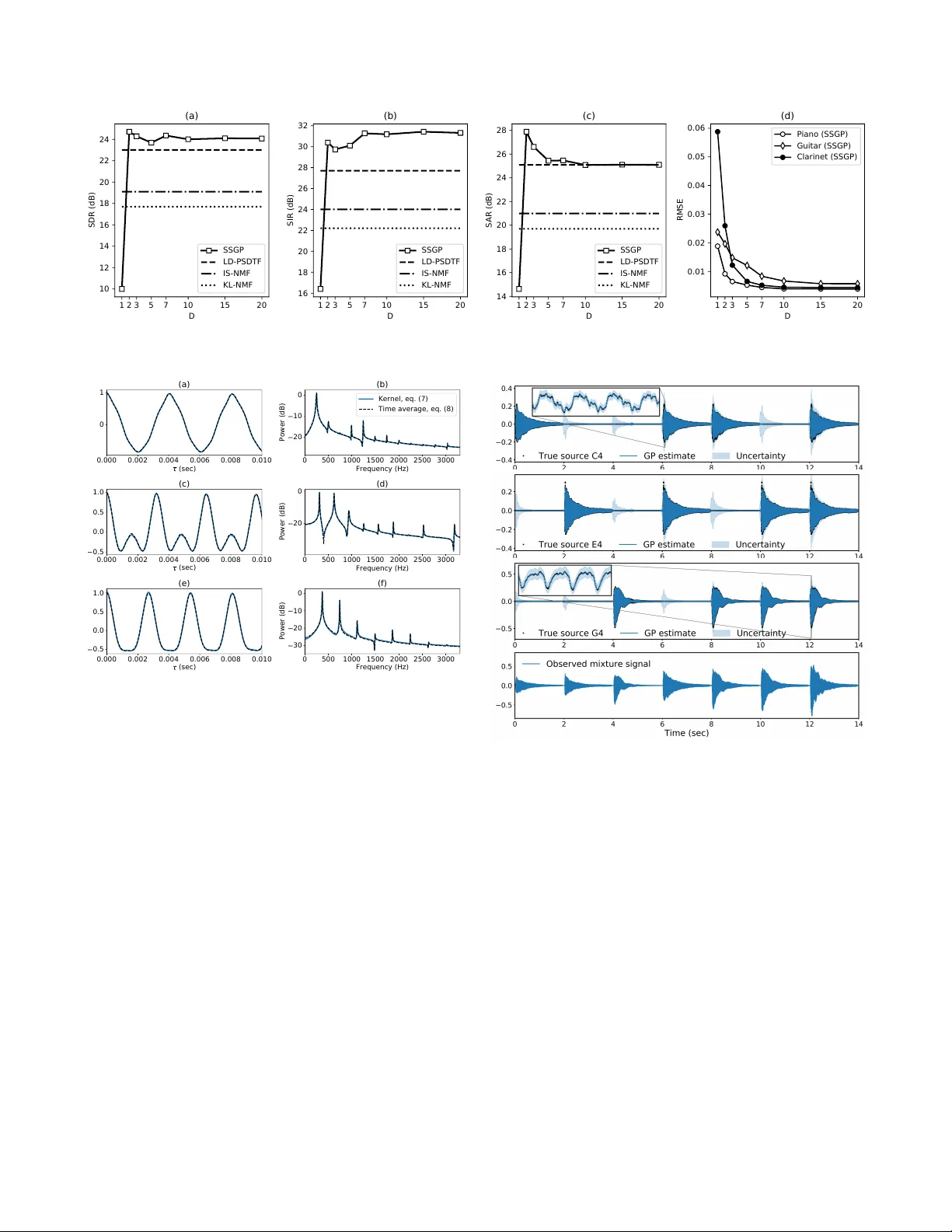
SP ARSE GA USSIAN PR OCESS A UDIO SOURCE SEP ARA TION USING SPECTR UM PRIORS IN THE TIME-DOMAIN P ablo A. Alvar ado ? ∗ Mauricio A. ´ Alvar ez § Dan Stowell ? † ? Centre for Digital Music, Queen Mary Uni versity of London, London, UK § Department of Computer Science, The Uni versity of Shef field, Sheffield, UK ABSTRA CT Gaussian process (GP) audio source separation is a time- domain approach that circumvents the inherent phase approx- imation issue of spectrogram based methods. Furthermore, through its kernel, GPs elegantly incorporate prior kno wl- edge about the sources into the separation model. Despite these compelling adv antages, the computational complexity of GP inference scales cubically with the number of audio samples. As a result, source separation GP models ha ve been restricted to the analysis of short audio frames. W e intro- duce an efficient application of GPs to time-domain audio source separation, without compromising performance. For this purpose, we used GP regression, together with spectral mixture kernels, and variational sparse GPs. W e compared our method with LD-PSDTF (positive semi-definite tensor factorization), KL-NMF (K ullback-Leibler non-negati ve ma- trix f actorization), and IS-NMF (Itakura-Saito NMF). Results show that the proposed method outperforms these techniques. Index T erms — T ime-domain source separation, Gaus- sian processes, spectral mixture kernels, variational inference. 1. INTR ODUCTION Single-channel audio source separation is a central problem in signal processing research. Here, the task is to estimate a certain number of latent signals or sources that were mixed together in one recorded mixture signal [1]. State of the art time-frequency methods for source separation include non- negati ve matrix factorisation (NMF) [2], and probabilistic la- tent component analysis (PLCA) [3]. These approaches de- compose the po wer spectrogram of the mixture into elemen- tary components. Then, the components are used to calculate the individual source-spectrograms. Time-frequenc y meth- ods often arbitrarily discard phase information. As a result, the phase of each source-spectrogram must be approximated, corrupting the reconstructed sources. In contrast, time-domain source separation approaches can av oid the phase approximation issue of time-frequency methods [4, 5]. For example, Y oshii et al. [6] reconstructed ∗ Supported by Colciencias scholarship 679. † Supported by EPSRC Fellowship EP/L020505/1. source signals from the mixture wa veform directly in the time domain. T o this end, Gaussian processes (GPs) were used to predict each source wa veform. GPs are probability distributions over functions [7]. A Gaussian process is com- pletely defined by a mean function, and a k ernel or cov ariance function. In fact, the kernel determines the properties of the functions sampled from a GP . A particularly influential w ork in time domain approaches is Liutkus et al. [1], who first formulated source separation as a GP regression task. Although source separation Gaussian process (SSGP) models circumv ent phase approximation, the computational complexity of GP inference scales cubically with the number of audio samples. Hence, different approximate techniques hav e been proposed to make the separation tractable. For instance, various authors partitioned the mixture signal into independent frames [1, 6]. Further , approximate inference in the frequency domain was used to learn model hyperparam- eters [1]. Alternativ ely , Adam et al. [8] recently proposed to use variational sparse GPs for source separation, howe ver audio signals were beyond the scope of their study . V aria- tional approaches rely on a set of inducing variables to build a low-rank approximation of the full cov ariance matrix. Here, the approximate distribution and hyperparameters are learned together by maximising a lower bound of the true marginal likelihood [9]. Moreov er , v ariational inference has allowed the application of GPs models to large datasets [10, 11]. Despite the kernel selection in SSGP models determines the properties of sources, only standard cov ariance functions hav e been used so f ar . For example, Adam et al. [8] consid- ered stationarity , smoothness and periodicity , using exponen- tiated quadratic times cosine kernels. Standard periodic ker- nels [12] were applied in [1]. These kernels assume that the source spectrum is composed of a fundamental frequency and perfect harmonics. Ho wever , real audio signals hav e more in- tricate spectra [13], and so separating audio sources requires more flexible cov ariance functions. One such covariance, the spectral mixture (SM) kernel [14], is intended for intricate spectrum patterns. SM k ernels approximate the spectral den- sity of any stationary cov ariance function, using a Gaussian mixture. Alternati vely , non-parametric kernels are implicitly considered when the cov ariance matrix of each source is di- rectly optimised by maximum likelihood [6]. Ho wever , that study did not contemplate variational sparse GPs. T o our knowledge, it has not been determined whether incorporating SM kernels together with variational sparse GPs into source separation models leads to more efficient and accurate audio source reconstructions. In this paper we introduce a method that combines GP re- gression [7, 1], spectral mixture kernels [14], and variati onal sparse GPs [9]. W e consider the mixture data as noisy obser - vations of a function of time, composed as the sum of a known number of sources. Further , we assume that each source fol- lows a different GP with a distinctiv e spectral mixture kernel. In addition, we adapt the kernels to reflect prior kno wledge about the typical spectral content of each source. Also, we frame the mixture data, and for ev ery frame we maximize a variational lower bound of the true mar ginal likelihood to learn the hyperparameters that control the amplitude of each source. Finally , to separate the sources, we use the learned priors to calculate the true posterior ov er each source. 2. GA USSIAN PR OCESS SOURCE SEP ARA TION W e notate the mixture data as y = [ y i ] n i =1 at time instants t = [ t i ] n i =1 . As mentioned previously , we consider each mix- ture audio sample y i as an observation of a mixture function f ( t ) corrupted by independent Gaussian noise. Further, we assume f ( t ) as the sum of J independent source functions { s j ( t ) } J j =1 . These functions represent the sources to be re- constructed. Each source s j ( t ) follo ws a dif ferent GP with zero mean, and a distinctive spectral mixture kernel. That is, y i = f ( t i ) +  i , where f ( t ) = P J j =1 s j ( t ) , and s j ( t ) ∼ G P ( 0 , k j ( t, t 0 ) ) for j = 1 , 2 , . . . , J. (1) Here, the noise follows  i ∼ N (0 , ν 2 ) , with v ariance ν 2 . The kernel for the j -th source is represented by k j ( t, t 0 ) (in- troduced shortly in section 2.1). In addition, it is a well known property that the sum of GPs is also a Gaussian process [7]. Therefore, the mixture function follows f ( t ) ∼ G P   0 , J X j =1 k j ( t, t 0 )   , (2) where its kernel is the sum of source kernels, i.e. k f ( t, t 0 ) = P J j =1 k j ( t, t 0 ) . W e focus only on predicting the mixture func- tion (2) as well as the sources (1) ev aluated at t . Any finite set of ev aluations of a GP function follows a multiv ariate normal distrib ution [7]. Therefore, the prior o ver the mixture function, and each source ev aluated at t , corre- spond to f ∼ N ( 0 , K f ) , and s j ∼ N  0 , K s j  respec- tiv ely , where the column vectors f = [ f ( t 1 ) , . . . , f ( t n )] > , s j = [ s j ( t 1 ) , . . . , s j ( t n )] > , and the covariance matrix K f = P J j =1 K s j . The matrices  K s j  J j =1 are computed by ev aluating the source kernels at all pair of time instants. That is, K s j [ l, l 0 ] = k j ( t l , t l 0 ) for l = 1 , 2 , . . . , n , and l 0 = 1 , 2 , . . . , n . Also, when a Gaussian likelihood is as- sumed, the priors are conjugate to the likelihood [7]. Hence, the posterior distributions are also Gaussian. That is, y | f ∼ n Y i =1 N  y i | f i , ν 2  , (3) f | y ∼ N  f | K > f H − 1 y , ˆ K f  , (4) s j | y ∼ N  s i | K > s j H − 1 y , ˆ K s j  . (5) Here, the likelihood (3) factorizes across the mixture data, and the posterior ov er the mixture function (4) has cov ari- ance matrix ˆ K f = K f − K > f H − 1 K f . Also, the posterior distribution over the i -th source (5) has covariance matrix ˆ K s j = K s j − K > s j H − 1 K s j , where the matrix H = K f + ν 2 I , and I is the identity matrix. Further, the model hyperparame- ters are usually learned by maximizing the log-marginal lik e- lihood log p ( y ) = − 1 2  y > H − 1 y + log | H | + n log 2 π  , (6) where H needs to be in verted. Although the source separation GP model introduced so far is elegant, its application to large audio signals becomes intractable. This is because the computational complexity of GP inference scales cubically with the number of audio samples. Specifically , learning the hyperparameters by max- imizing the true marginal likelihood (6) is computationally demanding, as it requires the inv ersion of a n × n matrix. T o overcome the limitations imposed by matrix in version, we instead maximized a variational lower bound of the true marginal lik elihood (6) (introduced shortly in section 2.2). In addition, we divided the mixture data into overlapping frames of size ˆ n  n . Finally , to reconstruct the sources, we used the hyperparameters learned for each frame to calculate the true posterior distribution ov er the sources (eq. (5)). The rest of this section is structured as follows. Section 2.1 intro- duces the spectral mixture k ernel used for each source. Then, section 2.2 presents the lower bound of the true marginal likelihood we maximized for learning the hyperparameters. 2.1. Spectral mixture kernels for isolated sources The kernel k j ( t, t 0 ) in (1) determines the properties of each source s j ( t ) , that is, smoothness, stationarity , and more im- portantly , its spectrum. T o model the typical spectral content of each isolated source, we used spectral mixture kernels [14]. These kernels approximate the spectral density of any station- ary cov ariance function using a Gaussian mixture. Further , Alvarado et al. [15] assumed a Lorentzian mixture instead, resulting in the Mat ´ ern- 1 / 2 spectral mixture (MSM) kernel k j ( τ ) = σ 2 j exp  − τ ` j  × D X d =1 α 2 j d cos( ω j d τ ) , (7) where τ = | t − t 0 | , the set of parameters n α 2 j d , ω j d o D d =1 controls the energy distribution throughout all the harmon- ics/partials of the j -th source spectrum. In addition, the variance σ 2 j controls the source amplitude, whereas the lengthscale ` j determines how fast s j ( t ) ev olves in time. W e grouped all the kernel parameters in the set θ j =  σ 2 j , ` j , n α 2 j d , ω j d o D d =1  . W e fitted a MSM kernel (7) to the spectrum of e very source. For this purpose, we used training data consisting of one audio recording of each iso- lated source. W e denoted the training data as  g ( j )  J j =1 , where g ( j ) = [ g ( j ) ( x i )] ˜ n i =1 is the training data vector for the j -th source, and x = [ x i ] ˜ n i =1 is the corresponding time vector . In addition, because only one single realization g ( j ) was av ailable for each source in { s j ( t ) } J j =1 , we assumed the sources to be cov ariance-ergodic processes with zero mean [16, 17, 18]. Therefore, their cov ariances { C j ( λ ) } J j =1 were estimated as the time av erage C j ( ˆ τ ) = 1 T Z T 0 g ( j ) ( x + ˆ τ ) g ( j ) ( x ) d x. (8) Here, T denotes the size (in seconds) of the window used to compute the correlation. W e used the discrete version of eq. (8). Finally , for every source we then minimized the mean square error (MSE) between the cov ariance estimator (8) and the corresponding MSM kernel (7). That is, L ( θ j ) = 1 N c N c X i =1 [ k j ( ˆ τ i ) − C j ( ˆ τ i )] 2 , (9) where N c is the number of points where (8) was approxi- mated, and θ j is the set of kernel parameters in (7). 2.2. Preprocessing and inference T o reduce the computational complexity of learning the hy- perparameters by maximizing the true marginal likelihood (6), we divided the mixture data { t i , y i } n i =1 into W overlap- ping frames of size ˆ n  n . Therefore, the set of frames corresponded to  ˆ t ( w ) , ˆ y ( w )  W w =1 . In addition, for each mix- ture frame ˆ y ( w ) , we instead maximized the lower bound of the true marginal likelihood, proposed by T itsias [9] for variational sparse GPs. This method depends on a smaller set of inducing variables u ∈ R m , where m ≤ ˆ n . The set u represents the values of the function f ( t ) (eq. (2)) ev aluated at a set of inducing points z = [ z i ] m i =1 . Thus, u = [ f ( z 1 ) , . . . , f ( z m )] > . The inducing points z lie on the same domain as t , i.e. time. Moreover , the inducing points, together with the model hyperparameters are learned by min- imizing the Kullback-Leibler (KL) di ver gence between the Gaussian approximate distrib ution q ( u ) , and the true poste- Method SDR SIR SAR Opt. time KL-NMF 17.7 22.2 19.7 – IS-NMF 19.1 24.0 21.0 – LD-PSDTF 23.0 27.7 25.1 – SSGP (proposed) 24.1 31.4 25.1 5.33 SSGP- full 22.9 22.3 24.6 284.2 T able 1 . Separation metrics (dB). Optimization time (min). rior p ( ˆ f | ˆ y ( w ) ) . This approach leads to the following bound L ∆ = log N  ˆ y ( w ) | 0 , Q ˆ n ˆ n + ν 2 I  − 1 2 ν 2 tr ( K ˆ n ˆ n − Q ˆ n ˆ n ) , (10) where the matrix Q ˆ n ˆ n = K ˆ nm K − 1 mm K m ˆ n . Here, the cross cov ariance K ˆ nm [ i, j ] = k f ( t ( w ) i , z j ) . Similarly , K mm [ i, j ] = k f ( z i , z j ) . Where t ( w ) i = t ( w ) [ i ] . Recall that k f ( t, t 0 ) is the kernel of the mixture function (eq. (2)). In brief, the computa- tional complexity of learning hyperparameters in each frame was reduced from O ( ˆ n 3 ) , to O ( ˆ nm 2 ) . 3. EXPERIMENT AL EV ALU A TION W e tested the proposed SSGP method on the same dataset analysed in [6]. That is, three different mixture audio signals sampled at 16 KHz, corresponding to piano, electric guitar , and clarinet. Each mixture lasts 14 seconds, and consists of the following sequence of music notes (C4, E4, G4, C4+E4, C4+G4, E4+G4, and C4+E4+G4). Thus, for each mixture, the aim was to reconstruct three source signals, each with a corresponding note, C4, E4, and G4. The metrics used to measure the separation performance were: source to distor- tion ratio (SDR), source to interferences ratio (SIR), source to artifacts ratio (SAR) [19], and root mean square error (RMSE). W e compared with LD-PSDTF (positiv e semi- definite tensor factorization), KL-NMF (Kullback-Leibler NMF), and IS-NMF (Itakura-Saito NMF) [6]. The code was implemented using GPflow [20]. W e determined the performance of the proposed method in mixtures of three sources. That is, J = 3 in eq. (2). T o this end, we first di vided the mixtures into frames of 125 mil- liseconds ( ˆ n = 2001 ) with 50% o verlap, and initialized the kernel for each source (eq. (7) with D = 15 ), by minimizing eq. (9). Then, for each mixture frame, we maximized eq. (10) to learn the variance of each source, i.e.,  σ 2 j  J j =1 . W e used two separate criteria to select z : either the inducing points were located at the extrema of the mixture data (sparse GP), or the inducing points were equal to the time v ector (full GP). W e compared the time required for learning the hyperparam- eters in these two scenarios. Finally , we used eq. (5), and the learned hyperparameters to calculate the true posterior over each source p  s ( w ) i | y ( w )  . W e recov ered the sources ap- plying the overlap - add method to the frame-wise predictions 1 2 3 5 7 10 15 20 D 10 12 14 16 18 20 22 24 SDR (dB) (a) SSGP LD-PSDTF IS-NMF KL-NMF 1 2 3 5 7 10 15 20 D 16 18 20 22 24 26 28 30 32 SIR (dB) (b) SSGP LD-PSDTF IS-NMF KL-NMF 1 2 3 5 7 10 15 20 D 14 16 18 20 22 24 26 28 SAR (dB) (c) SSGP LD-PSDTF IS-NMF KL-NMF 1 2 3 5 7 10 15 20 D 0.01 0.02 0.03 0.04 0.05 0.06 RMSE (d) Piano (SSGP) Guitar (SSGP) Clarinet (SSGP) Fig. 1 . Source separation metrics. SDR (a), SIR (b), SAR (c), RMSE (d). 0.000 0.002 0.004 0.006 0.008 0.010 (sec) 0 1 (a) 0 500 1000 1500 2000 2500 3000 Frequency (Hz) 20 10 0 Power (dB) (b) Kernel, eq. (7) Time average, eq. (8) 0.000 0.002 0.004 0.006 0.008 0.010 (sec) 0.5 0.0 0.5 1.0 (c) 0 500 1000 1500 2000 2500 3000 Frequency (Hz) 20 0 Power (dB) (d) 0.000 0.002 0.004 0.006 0.008 0.010 (sec) 0.5 0.0 0.5 1.0 (e) 0 500 1000 1500 2000 2500 3000 Frequency (Hz) 30 20 10 0 Power (dB) (f) Fig. 2 . Kernels learned for piano notes (left column). Corre- sponding log-spectral density (right column). [21]. W e found that our method (SSGP) presented the highest SDR and SIR metrics, and reduced the optimization time by 98.12% compared to the full GP (T able 1), indicating that our method is ef ficient, robust to interferences between sources (highest SIR), and it introduces less distortion (highest SDR). Further , we observed that the kernels learned for each source presented distinctiv e spectral patterns (Fig 2), which demon- strates that SM kernels are appropriate for learning the rich frequency content found in audio sources. Moreover , we ob- served that the proposed approach reconstructed accurately the sources (Fig 3), showing the variances learned by maxi- mizing the lower bound were consistent with the true sources. In addition, to establish the effect of kernel selection on the separation performance, we carried out the same previous ex- periment, but changing the number of components D in the kernel eq. (7). W e found that SDR, SIR and SAR metrics stabilized when D > 3 (Fig. 1(a-c)), indicating that the pro- posed model is less af fected by kernel selection when more than three components are used. Further , RMSE decreased exponentially with D (Fig. 1(d)), suggesting that increasing Fig. 3 . Source reconstruction on piano mixture signal. the number of components in the kernel leads to more accu- rate wa veform reconstructions. 4. CONCLUSIONS Our findings indicate that combining variational sparse GPs together with SM kernels enables time-domain source sepa- ration GP models to reconstruct audio sources in an efficient and informed manner , without compromising performance. Also, RMSE results imply that suitable spectrum priors over the sources are essential to improve source reconstruction. Moreov er , SDR, SIR, and SAR results suggest the proposed method can be used for other applications such as multipitch- detection, where low interference between sources (SIR) is more rele v ant than reconstruction artifacts (SAR). W e pro- posed an alternative method that circumvents phase approx- imation by addressing audio source separation from a varia- tional time-domain perspecti ve. The code is a v ailable at [22]. 5. REFERENCES [1] Antoine Liutkus, Roland Badeau, and G ¨ ael Richard, “Gaussian processes for underdetermined source sepa- ration, ” IEEE T ransactions on Signal Pr ocessing , vol. 59, no. 7, pp. 3155–3167, July 2011. [2] Daniel D. Lee and H. Sebastian Seung, “ Algorithms for non-negati ve matrix factorization, ” in Advances in Neural Information Processing Systems 13 (NIPS) , pp. 556–562. MIT Press, 2001. [3] Paris Smaragdis and Bhiksha Raj, “Shift-in variant prob- abilistic latent component analysis, ” T ech. Rep., Mit- subishi Electric Research Laboratories, 2007. [4] C ´ edric F ´ evotte and Matthieu K o walski, “Low-rank time-frequency synthesis, ” in Advances in Neur al Infor - mation Processing Systems 27 (NIPS) , pp. 3563–3571. Curran Associates, Inc., 2014. [5] Daniel Stoller, Sebastian Ewert, and Simon Dixon, “W av e-U-Net: A multi-scale neural network for end- to-end source separation, ” in International Society for Music Information Retrieval Conference (ISMIR) , 2018, vol. 19, pp. 334–340. [6] Kazuyoshi Y oshii, Ryota T omioka, Daichi Mochihashi, and Masataka Goto, “Beyond NMF: T ime-domain au- dio source separation without phase reconstruction, ” in 14th International Society for Music Information Re- trieval Confer ence (ISMIR) , 2013, pp. 369–374. [7] Carl Edward Rasmussen and Christopher K.I. W illiams, Gaussian Pr ocesses for Machine Learning (Adaptive Computation and Machine Learning) , The MIT Press, 2005. [8] V incent Adam, James Hensman, and Maneesh Sahani, “Scalable transformed additiv e signal decomposition by non-conjugate Gaussian process inference, ” in 26th IEEE International W orkshop on Machine Learning for Signal Pr ocessing (MLSP) , 2016, pp. 1–6. [9] Michalis K. T itsias, “V ariational learning of inducing variables in sparse Gaussian processes, ” in 12th Interna- tional Conference on Artificial Intelligence and Statis- tics (AIST A TS) , 2009, pp. 567–574. [10] James Hensman, Nicol ´ o Fusi, and Neil D. Lawrence, “Gaussian processes for big data, ” in 20th Confer ence on Uncertainty in Artificial Intelligence (UAI) , 2013, pp. 282–290. [11] James Hensman, Nicolas Durrande, and Arno Solin, “V ariational fourier features for Gaussian processes, ” Journal of Machine Learning Resear ch , vol. 18, no. 151, pp. 1–52, 2018. [12] David J. C. MacKay , “Introduction to Gaussian pro- cesses, ” in Neural Networks and Machine Learning , C. M. Bishop, Ed., N A TO ASI Series, pp. 133–166. Kluwer Academic Press, 1998. [13] T aylor Berg-Kirkpatrick, Jacob Andreas, and Dan Klein, “Unsupervised transcription of piano music, ” in Advances in Neural Information Pr ocessing Systems 27 (NIPS) , pp. 1538–1546. Curran Associates, Inc., 2014. [14] Andrew Gordon W ilson and Ryan Prescott Adams, “Gaussian process kernels for pattern discovery and ex- trapolation, ” 30th International Confer ence on Mac hine Learning (ICML) , pp. 1067–1075, 2013. [15] Pablo A. Alvarado and Dan. Stowell, “Ef ficient learn- ing of harmonic priors for pitch detection in polyphonic music, ” arXiv preprint , 2017. [16] Papoulis Athanasious, Pr obability , Random V ariables, and Stochastic Pr ocess , McGraw-Hill, Inc, 1991. [17] K. Sam Shanmugan and Arthur M. Breipohl, Random Signals: Detection, Estimation and Data Analysis , W i- ley , 1988. [18] M. Goulard and M. V oltz, “Linear coregionaliza- tion model: T ools for estimation and choice of cross- variogram matrix, ” Mathematical Geosciences , vol. 24, no. 3, pp. 269–286, 1992. [19] Emmanuel V incent, R ´ emi Gribon val, and C ´ edric F ´ evotte, “Performance measurement in blind audio source separation, ” IEEE T ransactions on Audio, Speech, and Language Pr ocessing , vol. 14, no. 4, pp. 1462–1469, July 2006. [20] Alexander G. de G. Matthe ws, Mark van der W ilk, T om Nickson, Keisuk e. Fujii, Alexis Boukouvalas, Pablo Le ´ on-V illagr ´ a, Zoubin Ghahramani, and James Hens- man, “GPflow: A Gaussian process library using T en- sorFlow , ” Journal of Machine Learning Researc h , vol. 18, no. 40, pp. 1–6, apr 2017. [21] J. B. Allen and L. R. Rabiner , “ A unified approach to short-time fourier analysis and synthesis, ” Proceedings of the IEEE , vol. 65, no. 11, pp. 1558–1564, No v 1977. [22] https://github.com/PabloAlvarado/ssgp .