Self-Attention Linguistic-Acoustic Decoder

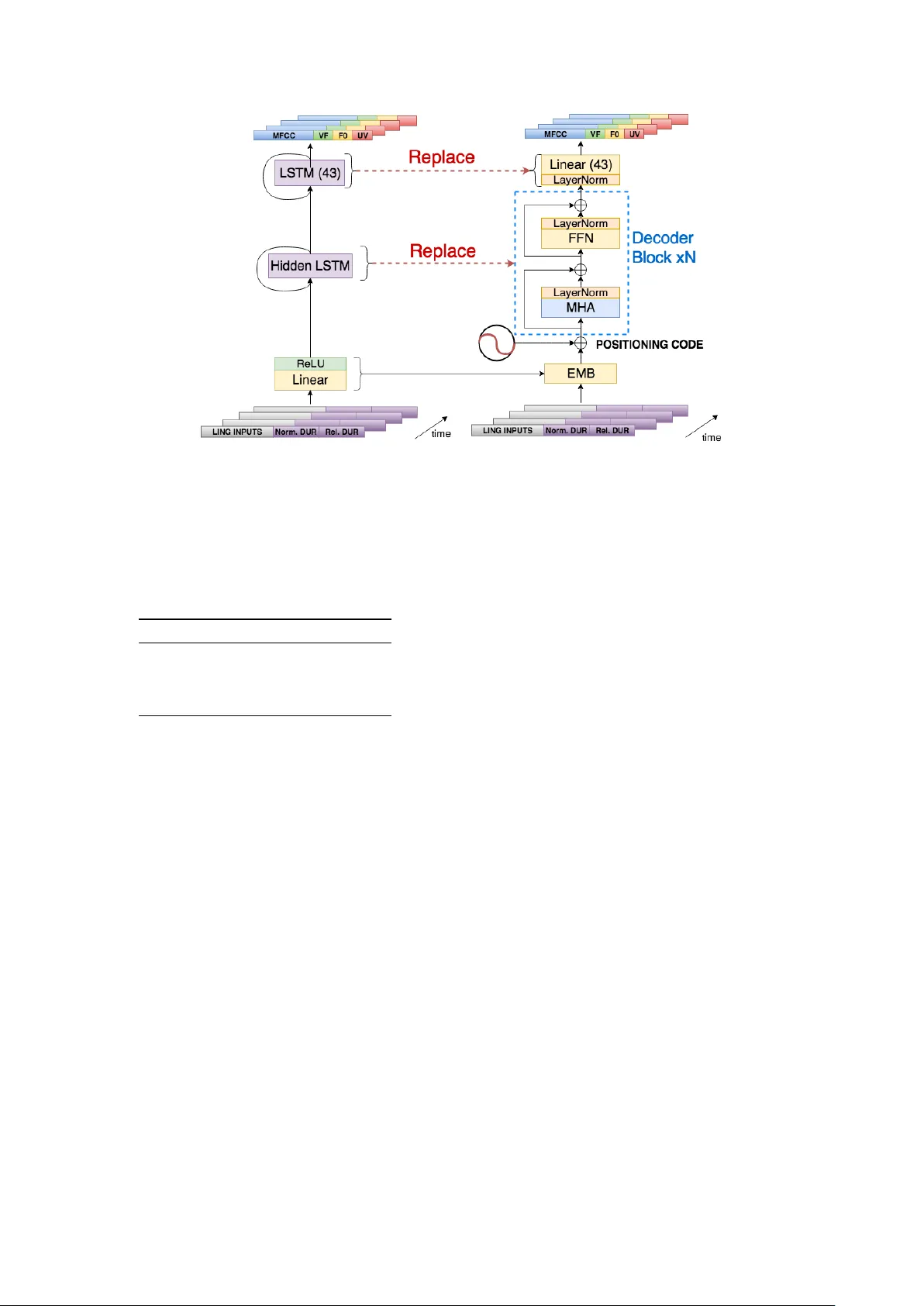
Self-Attention Linguistic-Acoustic Decoder Santiago P ascual 1 , Antonio Bonafonte 1 , J oan Serr ` a 2 1 Uni versitat Polit ` ecnica de Catalunya, Barcelona, Spain 2 T elef ´ onica Research, Barcelona, Spain santi.pascual@upc.edu Abstract The conv ersion from text to speech relies on the accurate map- ping from linguistic to acoustic symbol sequences, for which current practice employs recurrent statistical models like recur- rent neural networks. Despite the good performance of such models (in terms of low distortion in the generated speech), their recursi ve structure tends to make them slo w to train and to sample from. In this work, we try to overcome the limitations of recursiv e structure by using a module based on the transformer decoder network, designed without recurrent connections but emulating them with attention and positioning codes. Our re- sults show that the proposed decoder network is competitiv e in terms of distortion when compared to a recurrent baseline, whilst being significantly faster in terms of CPU inference time. On av erage, it increases Mel cepstral distortion between 0.1 and 0.3 dB, but it is over an order of magnitude faster on a verage. Fast inference is important for the deployment of speech syn- thesis systems on de vices with restricted resources, like mobile phones or embedded systems, where speaking virtual assistants are gaining importance. Index T erms : self-attention, deep learning, acoustic model, speech synthesis, text-to-speech. 1. Introduction Speech synthesis makes machines generate speech signals, and text-to-speech (TTS) conditions speech generation on input lin- guistic contents. Current TTS systems use statistical models like deep neural networks to map linguistic/prosodic features extracted from text to an acoustic representation. This acoustic representation typically comes from a v ocoding process of the speech wav eforms, and it is decoded into wav eforms again at the output of the statistical model [1]. T o build the linguistic to acoustic mapping, deep network TTS models make use of a two-stage structure [2]. The first stage predicts the number of frames (duration) of a phoneme to be synthesized with a duration model, whose inputs are lin- guistic and prosodic features extracted from text. In the second stage, the acoustic parameters of every frame are estimated by the so-called acoustic model. Here, linguistic input features are added to the phoneme duration predicted in the first stage. Dif- ferent works use this design, outperforming previously e xisting statistical parametric speech synthesis systems with different variants in prosodic and linguistic features, as well as perceptual losses of different kinds in the acoustic mapping [3, 4, 5, 6, 7]. Since speech synthesis is a sequence generation problem, re- current neural networks (RNNs) are a natural fit to this task. They have thus been used as deep architectures that effecti vely predict either prosodic features [8, 9] or duration and acoustic features [10, 11, 12, 13, 14]. Some of these works also investi- gate possible performance dif ferences using different RNN cell types, like long short-term memory (LSTM) [15] or gated re- current unit [16] modules. In this work, we propose a ne w acoustic model, based on part of the T ransformer network [17]. The original Trans- former was designed as a sequence-to-sequence model for ma- chine translation. T ypically , in sequence-to-sequence problems, RNNs of some sort were applied to deal with the con v ersion be- tween the two sequences [18, 19]. The T ransformer substitutes these recurrent components by attention models and positioning codes that act like time stamps. In [17], they specifically intro- duce the self-attention mechanism, which can relate elements within a single sequence without an ordered processing (like RNNs) by using a compatibility function, and then the order is imposed by the positioning code. The main part we import from that w ork is the encoder, as we are dealing with a mapping between two sequences that hav e the same time resolution. W e howe v er call this part the decoder in our case, gi ven that we are decoding linguistic contents into their acoustic codes. W e em- pirically find that this T ransformer netw ork is as competiti ve as a recurrent architecture, but with faster inference/training times. This paper is structured as follows. In section 2, we de- scribe the self-attention linguistic-acoustic decoder (SALAD) we propose. Then, in section 3, we describe the follo wed exper- imental setup, specifying the data, the features, and the hyper- parameters chosen for the overall architecture. Finally , results and conclusions are shown and discussed in sections 4 and 5, re- spectiv ely . The code for the proposed model and the baselines can be found in our public repository 1 . 2. Self-Attention Linguistic-Acoustic Decoder T o study the introduction of a Transformer network into a TTS system, we employ our previous multiple speaker adaptation (MUSA) framework [14, 20, 21]. This is a two-stage RNN model influenced by the w ork of Zen and Sak [13], in the sense that it uses unidirectional LSTMs to build the duration model and the acoustic model without the need of predicting dynamic acoustic features. A ke y dif ference between our works and [13] is the capacity to model many speakers and adapt the acoustic mapping among them with different output branches, as well as interpolating new voices out of their common representation. Nonetheless, for the current work, we did not use this multiple speaker capability and focused on just one speaker for the new architecture design on improving the acoustic model. The design differences between the RNN and the trans- former approaches are depicted in figure 1. In the MUSA framew ork with RNNs, we have a pre-projection fully- connected layer with a ReLU acti v ation that reduces the sparsity of linguistic and prosodic features. This embeds the mixture x t of different input types into a common representation h t in the 1 https://github .com/santi-pdp/musa tts form of one vector per time step t . Hence, the transformation R L → R H is applied independently at each time step t as h t = max(0 , Wx t + b ) , where W ∈ R H × L , b ∈ R H , x t ∈ R L , and h t ∈ R H . Af- ter this projection, we have the recurrent core formed by an LSTM layer of size H and an additional LSTM output layer . The MUSA-RNN output is recurrent, as this prompted better results than using dynamic features to smooth cepstral trajecto- ries in time [13]. Based on the Transformer architecture [17], we propose a pseudo-sequential processing network that can leverage distant element interactions within the input linguistic sequence to pre- dict acoustic features. This is similar to what an RNN does, but discarding any recurrent connection. This will allow us to pro- cess all input elements in parallel at inference, hence substan- tially accelerating the acoustic predictions. In our setup, we do not face a sequence-to-sequence problem as stated previously , so we only use a structure like the T ransformer encoder which we call a linguistic-acoustic decoder . The proposed SALAD architecture begins with the same embedding of linguistic and prosodic features, followed by a positioning encoding system. As we have no recurrent struc- ture, and hence no processing order , this positioning encod- ing system will allow the upper parts of the network to locate their operating point in time, such that the network will know where it is inside the input sequence [17]. This positioning code c ∈ R H is a combination of harmonic signals of v arying fre- quency: c t, 2 i = sin  t/ 10000 2 i H  c t, 2 i +1 = cos  t/ 10000 2 i H  where i represents each dimension within H . At each time-step t , we ha ve a unique combination of signals that serv es as a time stamp, and we can expect this to generalize better to long se- quences than having an incremental counter that marks the po- sition relativ e to the beginning. Each time stamp c t is summed to each embedding h t , and this is input to the decoder core. The decoder core is b uilt with a stack of N blocks, depicted within the dashed blue rectangle in figure 1. These blocks are the same as the ones proposed in the decoder of [17], but we only have self-attention modules to the input, so it looks more like the T ransformer encoder . The most salient part of this type of block is the multi-head attention (MHA) layer . This applies h parallel self-attention layers, which can ha ve a more v ersatile feature e xtraction than a single attention layer with the possibil- ity of smoothing intra-sequential interactions. After the MHA comes the feed-forward network (FFN), composed of two fully- connected layers. The first layer expands the attended features into a higher dimension d ff , and this gets projected again to the embedding dimensionality H . Finally , the output layer is a fully-connected dimension adapter such that it can con v ert the hidden dimensions H to the desired amount of acoustic outputs, which in our case is 43 as discussed in section 3.2. As stated ear- lier , we may slightly de grade the quality of predictions with this output topology , as recurrence helps in the output layer captur - ing better the dynamics of acoustic features. Nonetheless, this can suf fice our objecti ve of having a highly parallelizable and competitiv e system. 3. Experimental Setup 3.1. Dataset For the experiments we use utterances of speakers from the TCST AR project dataset [22]. This corpora includes sentences and paragraphs taken from transcribed parliamentary speech and transcribed broadcast news. The purpose of these text sources is twofold: enrich the vocab ulary and facilitate the se- lection of the sentences to achieve good prosodic and phonetic cov erage. For this work, we choose the same male (M1) and fe- male (F1) speakers as in our previous works. These two speak- ers hav e the most amount of data among the av ailable ones. Their amount of data is balanced with approximately the fol- lowing durations per split for both: 100 minutes for training, 15 minutes for validation, and 15 minutes for test. 3.2. Linguistic and Acoustic Featur es The decoder maps linguistic and prosodic features into acous- tic ones. This means that we first extract hand-crafted features out of the input textual query . These are extracted in the la- bel format, following our previous work in [20]. W e thus hav e a combination of sparse identifiers in the form of one-hot vec- tors, binary v alues, and real v alues. These include the identity of phonemes within a window of context, part of speech tags, distance from syllables to end of sentence, etc. For more detail we refer to [20] and references therein. For a textual query of N words, we will obtain M label vectors, M ≥ N , each with 362 dimensions. In order to inject these into the acoustic decoder, we need an e xtra step though. As mentioned, the MUSA testbed follows the two-stage struc- ture: (1) duration prediction and (2) acoustic prediction with the amount of frames specified in first stage. Here we are only working with the acoustic mapping, so we enforce the duration with labeled data. For this reason, and similarly to what we did in pre vious works [14, 21], we replicate the linguistic label v ec- tor of each phoneme as many times as dictated by the ground- truth annotated duration, appending two extra dimensions to the 362 existing ones. These two extra dimensions correspond to (1) absolute duration normalized between 0 and 1, given the training data, and (2) relativ e position of current phoneme in- side the absolute duration, also normalized between 0 and 1. W e parameterize the speech with a v ocoded representa- tion using Ahocoder [23]. Ahocoder is an harmonic-plus-noise high quality vocoder , which con verts each windowed wav eform frame into three types of features: (1) mel-frequency cepstral coefficients (MFCCs), (2) log-F0 contour, and (3) voicing fre- quency (VF). Note that F0 contours ha ve tw o states: either they follow a continuous envelope for voiced sections of speech, or they are 0, for which the logarithm is undefined. Because of that, Ahocoder encodes this value with − 10 9 , to avoid numeri- cal undefined values. This result would be a cumbersome output distribution to be predicted by a neural net using a quadratic re- gression loss. Therefore, to smooth the values out and normal- ize the log-F0 distribution, we linearly interpolate these con- tours and create an extra acoustic feature, the unv oiced-voiced flag (UV), which is the binary flag indicating the voiced or un- voiced state of the current frame. W e will then ha ve an acoustic vector with 40 MFCCs, 1 log-F0, 1 VF , and 1 UV . This equals a total number of 43 features per frame, where each frame window has a stride of 80 samples over the wav eform. Real- numbered linguistic features are Z-normalized by computing statistics on the training data. In the acoustic feature outputs, all of them are normalized to fall within [0 , 1] . Figure 1: T ransition from RNN/LSTM acoustic model to SALAD. The embedding projections ar e the same. P ositioning encoding intr oduces sequential information. The decoder block is stacked N times to form the whole structur e r eplacing the recurr ent core . FFN: F eed-forward Network. MHA: Multi-Head Attention. T able 1: Differ ent layer sizes of the differ ent models. Emb: lin- ear embedding layer , and hidden size H for SALAD models in all layers but FFN ones. HidRNN: Hidden LSTM layer size. d ff : Dimension of the feed-forwar d hidden layer inside the FFN. Model Emb HidRNN d ff Small RNN 128 450 - Small SALAD 128 - 1024 Big RNN 512 1300 - Big SALAD 512 - 2048 3.3. Model Details and T raining Setup W e have two main structures: the baseline MUSA-RNN and SALAD. The RNN takes the form of an LSTM network for their known advantages of a voiding typical v anilla RNN pitfalls in terms of vanishing memory and bad gradient flo ws. Each of the two different models has two configurations, small (Small RNN/Small SALAD) and big (Big RNN/Big SALAD). This in- tends to show the performance difference with re gard to speed and distortion between the proposed model and the baseline, but also their variability with respect to their capacity (RNN and SALAD models of the same capacity hav e an equiv alent number of parameters although they hav e different connexion topologies). Figure 1 depicts both models’ structure, where only the size of their layers (LSTM, embedding, MHA, and FFN) changes with the mentioned magnitude. T able 1 sum- marizes the different layer sizes for both types of models and magnitudes. Both models hav e dropout [24] in certain parts of their structure. The RNN models have it after the hidden LSTM layer , whereas the SALAD model has many dropouts in dif fer- ent parts of its submodules, replicating the ones proposed in the original T ransformer encoder [17]. The RNN dropout is 0.5, and SALAD has a dropout of 0.1 in its attention components and 0.5 in FFN and after the positioning codes. Concerning the training setup, all models are trained with batches of 32 sequences of 120 symbols. The training is in a so-called stateful arrangement, such that we carry the sequen- tial state between batches over time (that is, the memory state in the RNN and the position code inde x in SALAD). T o achie ve this, we concatenate all the sequences into a very long one and chop it into 32 long pieces. W e then use a non-overlapped slid- ing window of size 120, so that each batch contains a piece per sequence, continuous with the pre vious batch. This makes the models learn ho w to deal with sequences longer than 120 out- side of train, learning to use a conditioning state different than zero in training. Both models are trained for a maximum of 300 epochs, but they trigger a break by early-stopping with the validation data. The validation criteria for which they stop is the mel cepstral distortion (MCD; discussed in section 4) with a patience of 20 epochs. Regarding the optimizers, we use Adam [25] for the RNN models, with the default parameters in PyT orch (lr = 0 . 001 , β 1 = 0 . 9 , β 2 = 0 . 999 , and  = 10 − 8 ). For SALAD we use a variant of Adam with adaptive learning rate, already proposed in the T ransformer work, called Noam [17]. This optimizer is based on Adam with β 1 = 0 . 9 , β 2 = 0 . 98 ,  = 10 − 9 and a learning rate scheduled with lr = H − 0 . 5 · min( s − 0 . 5 , s · w − 1 . 5 ) where we have an increasing learning rate for w warmup train- ing batches, and it decreases afterwards, proportionally to the in verse square root of the step number s (number of batches). W e use w = 4000 in all experiments. The parameter H is the inner embedding size of SALAD, which is 128 or 512 depend- ing on whether it is the small or big model as noted in table 1. W e also tested Adam on the big version of SALAD, but we did not observe any improv ement in the results, so we stick to Noam following the original T ransformer setup. T able 2: Male (top) and female (bottom) objective results. A: voiced/un voiced accuracy . Model #Params MCD [dB] F0 [Hz] A [%] Small RNN 1.17 M 5.18 13.64 94.9 Small SALAD 1.04 M 5.92 16.33 93.8 Big RNN 9.85 M 5.15 13.58 94.9 Big SALAD 9.66 M 5.43 14.56 94.5 Small RNN 1.17 M 4.63 15.11 96.8 Small SALAD 1.04 M 5.25 20.15 96.4 Big RNN 9.85 M 4.73 15.44 96.9 Big SALAD 9.66 M 4.84 19.36 96.6 4. Results In order to assess the distortion introduced by both models, we took three different objecti ve e valuation metrics. First, we hav e the MCD measured in decibels, which tells us the amount of distortion in the prediction of the spectral en velope. Then we hav e the root mean squared error (RMSE) of the F0 prediction in Hertz. And finally , as we introduced the binary flag that spec- ifies which frames are voiced or unv oiced, we measure the accu- racy (number of correct hits over total outcomes) of this binary classification prediction, where classes are balanced by nature. These metrics follow the same formulations as in our pre vious works [14, 20, 21]. T able 2 shows the objecti ve results for the systems detailed in section 3.3 ov er the two mentioned speakers, M and F . For both speakers, RNN models perform better than the SALAD ones in terms of accuracy and error . Even though the small- est gap, occurring with the SALAD biggest model, is 0.3 dB in the case of the male speaker and 0.1 dB in the case of the female speaker , showing the competiti ve performance of these non-recurrent structures. On the other hand, Figure 3 depicts the inference speed on CPU for the 4 dif ferent models synthe- sizing different utterance lengths. Each dot in the plot indicates a test file synthesis. After we collected the dots, we used the RANSA C [26] algorithm (Scikit-learn implementation) to fit a linear regression robust to outliers. Each model line shows the latency uprise trend with the generated utterance length, and RNN models have a way higher slope than the SALAD models. In fact, SALAD models remain pretty flat ev en for files of up to 35 s, having a maximum latency in their linear fit of 5.45 s for the biggest SALAD, whereas ev en small RNN is ov er 60 s. W e ha ve to note that these measurements are taken with Py- T orch [27] implementations of LSTM and other layers running ov er a CPU. If we run them on GPU we notice that both systems can work in real time. It is true that SALAD is still faster ev en in GPU, howe ver the big gap happens on CPUs, which motiv ates the use of SALAD when we hav e more limited resources. W e can also check the pitch prediction deviation, as it is the most affected metric with the model change. W e show the test pitch histograms for ground truth, big RNN and big SALAD in figure 2. There we can see that SALAD’ s failure is about focusing on the mean and ignoring the variance of the real dis- tribution more than the RNN does. It could be interesting to try some sort of short-memory non-recurrent modules close to the output to alle viate this peaky beha vior that makes pitch flat- ter (and thus less expressi ve), checking if this is directly re- lated to the removal of the recurrent connection in the output layer . Audio samples are av ailable online as qualitativ e results at http://veu.talp.cat/saladtts . Figure 2: F0 contour histogr ams of gr ound-truth speech, bi- gRNN and bigSALAD for male speaker . Figure 3: Infer ence time for the four differ ent models with re- spect to generated waveform length. Both axis ar e in seconds. T able 3: Maximum infer ence latency with RANSAC fit. Model Max. latency [s] Small RNN 63.74 Small SALAD 4.715 Big RNN 64.84 Big SALAD 5.455 5. Conclusions In this work we present a competitiv e and fast acoustic model replacement for our MUSA-RNN TTS baseline. The proposal, SALAD, is based on the Transformer network, where self- attention modules build a global reasoning within the sequence of linguistic tokens to come up with the acoustic outcomes. Furthermore, positioning codes ensure the ordered processing in substitution of the ordered injection of features that RNN has intrinsic to its topology . With SALAD, we get on average ov er an order of magnitude of inference acceleration against the RNN baseline on CPU, so this is a potential fit for applying text- to-speech on embedded devices like mobile handsets. Further work could be dev oted on pushing the boundaries of this system to alleviate the observ ed flatter pitch behavior . 6. Acknowledgements This research was supported by the project TEC2015-69266-P (MINECO/FEDER, UE). 7. References [1] H. Zen, “ Acoustic modeling in statistical parametric speech synthesis–from HMM to LSTM-RNN, ” 2015. [2] H. Zen, A. Senior , and M. Schuster , “Statistical parametric speech synthesis using deep neural networks, ” in 2013 IEEE Interna- tional Confer ence on Acoustics, Speech and Signal Processing (ICASSP) . IEEE, 2013, pp. 7962–7966. [3] H. Lu, S. King, and O. W atts, “Combining a vector space rep- resentation of linguistic context with a deep neural network for text-to-speech synthesis, ” Proc. ISCA SSW8 , pp. 281–285, 2013. [4] Y . Qian, Y . Fan, W . Hu, and F . K. Soong, “On the training aspects of deep neural network (DNN) for parametric TTS synthesis, ” in 2014 IEEE International Confer ence on Acoustics, Speech and Signal Pr ocessing (ICASSP) . IEEE, 2014, pp. 3829–3833. [5] Q. Hu, Z. W u, K. Richmond, J. Y amagishi, Y . Stylianou, and R. Maia, “Fusion of multiple parameterisations for DNN-based sinusoidal speech synthesis with multi-task learning, ” in Pr oc. IN- TERSPEECH , 2015, pp. 854–858. [6] Q. Hu, Y . Stylianou, R. Maia, K. Richmond, J. Y amagishi, and J. Latorre, “ An inv estigation of the application of dynamic sinu- soidal models to statistical parametric speech synthesis. ” in Proc. INTERSPEECH , 2014, pp. 780–784. [7] S. Kang, X. Qian, and H. Meng, “Multi-distribution deep be- lief network for speech synthesis, ” in Pr oc. 2013 IEEE Interna- tional Confer ence on Acoustics, Speech and Signal Processing (ICASSP) . IEEE, 2013, pp. 8012–8016. [8] S. Pascual and A. Bonafonte, “Prosodic break prediction with RNNs, ” in Pr oc. International Confer ence on Advances in Speec h and Language T echnologies for Iberian Languages . Springer , 2016, pp. 64–72. [9] S.-H. Chen, S.-H. Hwang, and Y .-R. W ang, “ An RNN-based prosodic information synthesizer for mandarin text-to-speech, ” IEEE T ransactions on Speech and A udio Pr ocessing , vol. 6, no. 3, pp. 226–239, 1998. [10] S. Achanta, T . Godambe, and S. V . Gang ashetty , “ An in vestigation of recurrent neural network architectures for statistical parametric speech synthesis, ” in Pr oc. INTERSPEECH , 2015. [11] Z. W u and S. King, “In vestigating gated recurrent networks for speech synthesis, ” in Pr oc. International Confer ence on Acous- tics, Speech and Signal Pr ocessing (ICASSP) . IEEE, 2016, pp. 5140–5144. [12] R. Fernandez, A. Rendel, B. Ramabhadran, and R. Hoory , “Prosody contour prediction with long short-term memory , bi- directional, deep recurrent neural networks. ” in Proc. INTER- SPEECH , 2014, pp. 2268–2272. [13] H. Zen and H. Sak, “Unidirectional long short-term memory re- current neural network with recurrent output layer for lo w-latency speech synthesis, ” in Pr oc. International Confer ence on Acous- tics, Speech and Signal Pr ocessing (ICASSP) . IEEE, 2015, pp. 4470–4474. [14] S. P ascual and A. Bonafonte, “Multi-output RNN-LSTM for mul- tiple speaker speech synthesis and adaptation, ” in Proc. 24th Eu- r opean Signal Pr ocessing Conference (EUSIPCO) . IEEE, 2016, pp. 2325–2329. [15] S. Hochreiter and J. Schmidhuber , “Long short-term memory , ” Neural computation , v ol. 9, no. 8, pp. 1735–1780, 1997. [16] J. Chung, C. Gulcehre, K. Cho, and Y . Bengio, “Empirical ev alu- ation of gated recurrent neural networks on sequence modeling, ” arXiv pr eprint arXiv:1412.3555 , 2014. [17] A. V aswani, N. Shazeer, N. Parmar , J. Uszkoreit, L. Jones, A. N. Gomez, Ł. Kaiser, and I. Polosukhin, “ Attention is all you need, ” in Proc. Advances in Neural Information Pr ocessing Systems (NIPS) , 2017, pp. 6000–6010. [18] I. Sutskev er , O. V inyals, and Q. V . Le, “Sequence to sequence learning with neural networks, ” in Pr oc. Advances in Neural In- formation Pr ocessing Systems (NIPS) , 2014, pp. 3104–3112. [19] D. Bahdanau, K. Cho, and Y . Bengio, “Neural machine trans- lation by jointly learning to align and translate, ” arXiv pr eprint arXiv:1409.0473 , 2014. [20] S. Pascual, “Deep learning applied to speech synthesis, ” Master’ s thesis, Univ ersitat Polit ` ecnica de Catalunya, 2016. [21] S. Pascual and A. Bonafonte C ´ avez, “Multi-output RNN-LSTM for multiple speaker speech synthesis with a-interpolation model, ” in Pr oc. ISCA SSW9 . IEEE, 2016, pp. 112–117. [22] A. Bonafonte, H. H ¨ oge, I. Kiss, A. Moreno, U. Ziegenhain, H. van den Heuvel, H.-U. Hain, X. S. W ang, and M.-N. Garcia, “Tc-star: Specifications of language resources and evaluation for speech synthesis, ” in Pr oc. LREC Conf , 2006, pp. 311–314. [23] D. Erro, I. Sainz, E. Nav as, and I. Hern ´ aez, “Improved HNM- based vocoder for statistical synthesizers. ” in Proc. INTER- SPEECH , 2011, pp. 1809–1812. [24] N. Sriv astav a, G. Hinton, A. Krizhevsk y , I. Sutskev er , and R. Salakhutdinov , “Dropout: a simple way to prevent neural net- works from overfitting, ” The Journal of Machine Learning Re- sear ch , v ol. 15, no. 1, pp. 1929–1958, 2014. [25] D. P . Kingma and J. Ba, “ Adam: A method for stochastic opti- mization, ” arXiv pr eprint arXiv:1412.6980 , 2014. [26] M. A. Fischler and R. C. Bolles, “Random sample consensus: a paradigm for model fitting with applications to image analysis and automated cartography , ” Communications of the A CM , vol. 24, no. 6, pp. 381–395, 1981. [27] A. Paszke, S. Gross, S. Chintala, G. Chanan, E. Y ang, Z. De- V ito, Z. Lin, A. Desmaison, L. Antiga, and A. Lerer, “ Automatic differentiation in PyT orch, ” in NIPS W orkshop on The Future of Gradient-based Machine Learning Softwar e & T echniques (NIPS- Autodif f) , 2017.