Low-Dimensional Bottleneck Features for On-Device Continuous Speech Recognition

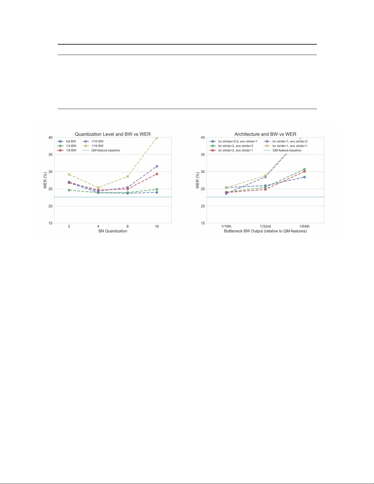
LO W -DIMENSIONAL BO TTLENECK FEA TURES FOR ON-DEVICE CONTINUOUS SPEECH RECOGNITION David B. Ramsay ? ∗ K evin Kilgour † Dominik Roblek † Matthew Sharifi † ? MIT Media Laboratory † Google AI ABSTRA CT Low power digital signal processors (DSPs) typically have a very limited amount of memory in which to cache data. In this paper we de velop efficient bottleneck feature (BNF) ex- tractors that can be run on a DSP, and retrain a baseline l arge- vocab ulary continuous speech recognition (L VCSR) system to use these BNFs with only a minimal loss of accuracy . The small BNFs allo w the DSP chip to cache more audio features while the main application processor is suspended, thereby reducing the overall battery usage. Our presented system is able to reduce the footprint of standard, fixed point DSP spec- tral features by a factor of 10 without any loss in word error rate (WER) and by a factor of 64 with only a 5 . 8 % relati ve increase in WER. Index T erms — bottleneck features, large v ocabulary con- tinuous speech recognition, low-po wer deep learning, mobile 1. INTR ODUCTION Large-v ocabulary continuous speech recognition (L VCSR) can be used to extract rich context about a user’ s interests, intents, and state. If run on a mobile device, this has the po- tential to rev olutionize the quality of on-device services they interact with. In order for this to become practical, hardware- lev el optimization is required to preserve the battery life of portable devices. In this paper , we present a ne w L VCSR model architecture that takes advantage of a low-po wer , fixed point, always-on digital signal processor (DSP) to significantly reduce power consumption. Our goal is to use the DSP to optimally com- press incoming speech into its bottleneck features (BNFs) representation which is cached for as long a period as possi- ble. By increasing the amount of cached input, we reduce t he wake-up frequency of the device’ s main processor, which is used to complete the inference. W e start with a state-of-the-art Listen, Attend, Spell (LAS) end-to-end automatic speech recognition (ASR) model, and ef fecti vely split its encoder across the DSP and the main processor . Hardware optimization across the DSP and main ∗ The first author performed this work while at Google AI. processor has been successfully lev eraged in the past to cache features for similar lo w-po wer services [1], though this is the first time that a DSP has been used to compute the initial lay- ers in the primary inference model. This leads to a significant increase in the amount of audio we can cache, with minimal impact to the model’ s overall WER. Furthermore, as a purely on-device model, this design preserves user priv acy as well as battery life. The topology is an important step towards practical L VCSR in highly po wer -constrained contexts. 2. RELA TED WORK Fully end-to-end L VCSR are emerging as the state-of-the-art [2], equalling and ev en surpassing the performance of stan- dard connectionist temporal classification [3] models. The core architecture for these end-to-end models, called Listen, Attend, and Spell [4], contains three major subgraphs - an encoder , an attention mechanism, and a decoder . Since their proposal in 2015, there has been a substantial amount of work done to optimize these models for on-device use [5], [6], in- cluding weight matrix factorization, pruning, and model dis- tillation. Due to these improvements, it is now possible to run a state-of-the-art L VCSR model on a mobile device’ s core processor (at a high power cost). For the traditional hidden markov model (HMM)-based systems that predate LAS architectures, neural networks (NN) had been heavily used as part of a traditional ASR acoustic model. V esel ` y, Karafi ´ at, and Gr ´ ezl [7] sho w that conv olu- tional bottleneck compression improv es system performance in such setups. T ypically , these compressed representations are concatenated with small time-window features to provide ’context’. Additionally , small HMM-based ke yword spotters have been successfully optimized across a DSP and main proces- sor . Shah, Arunachalam, W ang, et al. [8] propose a model which introduces 5 − and 6 bit weight quantization for a re- duced memory footprint without a significant reduction in ac- curacy . Although these models ha ve different architectures and applications, their use of con v olutional bottleneck fea- tures and fixed-point network quantization inform our archi- tecture. Fig. 1 : The default configuration of a bottlenec k layer running on the DSP; her e we see a kernel size of 4 applied in a frequency separable way , followed by one fr equency k ernel per output channel. These two con volutions are considered as a single ’layer’. Shah, Arunachalam, W ang, et al. [8], Gfeller, Guo, Kil- gour , et al. [1] introduce a split across a fixed-point DSP and a main processor motiv ated by power optimization. A quan- tized, tw o-stage, separable con volutional layer running on the DSP forms the basis of their music detector . W e use the same layer structure in our DSP implementation. The previously mentioned approaches do not attempt to compress audio features before caching, b ut there are other analyses of the trade-off between feature caching and power savings in the literature. In Priyantha, L ymberopoulos, and Liu [9] and Priyantha, L ymberopoulos, and Liu [10], empir- ical power consumption drops from 700 mW to 25 mW as data is cached 50 x longer for a pedometer application. Mea- surements of Gfeller, Guo, Kilgour, et al. [1] indicate a full 25 % - 50 % of the power cost at inference time is due to fixed wakeup and sleep ov erhead. Our goal is to significantly re- duce this fixed po wer cost. 3. FEA TURE SUBSTITUTION State-of-the-art results are reported in Chiu, Sainath, W u, et al. [2] with a very large, proprietary corpus. In this paper, we use the Librispeech 100 corpus to train our model [11]. Chiu, Sainath, W u, et al. [2] report a WER of 4 . 1 % with o ver 12,500 hours of training data; the same model trained on 100 hours of Librispeech data giv es a WER of 21 . 8 % , which we use as the baseline for all further ev aluation. The model from Chiu, Sainath, W u, et al. [2] is capable of running on a phone using 80-dimensional, 32 bit floating point mel spectrum audio features sampled in 25 ms windows ev ery 10 ms . These features capture a maximum frequency of 7 . 8 kHz and are stacked with delta and double delta fea- tures, resulting in an 80 x 3 input vector at each timestep. W e replace these features with quantized mel featur es (QM- featur es) that are compact, simple to calculate, and currently in use by other services running on the DSP. QM-features are log-mel based with a 16 bit fixed point representation. W e use a default, narro w-band frequency rep- resentation that only captures up to 3 . 8 Hz over 32 bins. W e test the effect of reducing the bandwidth by simply using fewer log-mel bins. Sampling rate and windo w size are con- stant across test input features and, for each case, we train an end-to-end model. The results of training a state-of-the-art LAS model with dif ferent input representations which can be calculated and cached on the DSP can be seen in T able 1. The results indicate that the baseline model, whose fea- tures have not previously been optimized, has a heavily re- dundant input representation, requiring three times the BW of the raw audio after delta stacking. W e are able to significantly reduce the input BW (and, by extension, the amount of com- putation in the initial LAS layers) without sev erely affecting the model’ s WER. Delta- and double delta- feature stacking do not have a large effect relativ e to their 3 x increase in size; thus we will take the standard 32 bin QM-features input as our starting point for further exploration. Though we see an incremental trade-off between BW and WER for smaller raw feature rep- resentations, we will use the full 32 bin QM-features as an input to our compressiv ed bottleneck layers in an attempt to preserve WER while reducing the BW e ven more drastically . 4. BO TTLENECK FEA TURE EXTRA CTION Our model uses the con volutional structure outlined by Gfeller, Guo, Kilgour , et al. [1]. The structure of a single layer is shown in Figure 1. These simple, separable con- volutional layers have been optimized for the DSP. Besides minimal computation, all layer weights and intermediate representations are quantized to 8 bits . 32 bit biases, batch normalization [13], and a restricted linear unit (ReLU) acti- vation function are included after the second, 1-D separable con volution. T o explore the space of bottleneck architectures, we pa- rameterized this architecture along the following axes: output dimension size, output quantization level, conv olutional stride (in time), kernel size, and the number of layers in the bottle- Model Input Input Dims Feature T ype WER (%) bandwidth (BW) (kbps) 16 kHz 16 bit raw PCM audio – – – 256 Baseline LAS Model 80 x 3 Mel, + ∆ + ∆∆ 21.79 768 Standard QM-features + Deltas 32 x 3 Mel, + ∆ + ∆∆ 22.42 154 Standard QM-features 32 x 1 Mel 22.62 51.2 3/4 BW QM-features 24 x 1 Mel 22.80 38.4 1/2 BW QM-features 16 x 1 Mel 22.97 25.6 1/4 BW QM-features 8 x 1 Mel 24.52 12.8 T able 1 : Comparison of model performance with smaller feature representations. Fig. 2 : The left plot uses a bottleneck feature extractor with a single hidden layer in which the output layer dimension and quantization lev el were modified to giv e a certain bandwidth output (relativ e to the standard 32 d imensional 16 bit QM-features). W e see a trend towards 4-bit quantization, especially at high compression lev- els. The right plot shows the performance of v arious architectures (dif ferent bottleneck and encoder depths/strides and BNF dimension) at 4-bit quantization, plotted against bandwidth. As more drastic compression is demanded, shifting the stride to before the BNFs improves performance, which is similar to reducing the frame rate in more traditional models [12]. neck network. The first three ax es ha ve the potential to reduce the BW of the resulting bottleneck, while the latter two axes are relev ant to the size of the resulting model. Reducing the output dimension size is equiv alent to reducing the size of the bottleneck layer and can result in a proportional reduction in BW. The output quantization level affects how many bits are sav ed for each of the v alues in the output, and will also result in a proportional reduction in BW. Increasing the stride could exponentially decrease the BW, for example, by doubling the stride we generate outputs only half as often. These changes in input lead to a necessary modification of the initial two con volutional layers of the LAS encoder , which are designed with 3x3 time-frequency kernels and strides of 2. W e replace these (by default) with a 3x1 time kernel along the flattened and modified frequency axis. W e also vary the number of initial encoder layers and strides in our analysis. 5. RESUL TS Initial results are based on freezing the bottleneck (BN) ex- tractor and encoder layer parameters and v arying one param- eter at time. This analysis re vealed a statistically insignificant effect of BN kernel size (across a range from 1 to 10) based on McNemar statistical tests [14]. Activ ation function com- parisons fav ored ReLU in a default configuration, but at high lev els of quantization/compression showed no difference be- tween identity and ReLU activ ation functions. There was a clear performance loss when increasing BN stride without a simultaneous decrease in encoder stride. W e hypothesize that the model has already been optimally com- pressed in the time dimension (the original model has a time step of 10 ms fed through two strides of two, resulting in an encoded frame every 40 ms ). No dependence on encoder depth was noticeable. In Figure 2, we see the results of varying the BNF output dimension and quantization le vel at dif ferent rates of com- Model # BNF Extractor W eights ∆ LAS Encoder W eights T otal Stride 1 BW (kbps) WER (%) 16kHz 16-bit Raw PCM Audio – – – 256 – Baseline LAS Model – 0 (0) 4 768 21.79 Standard QM-features 0 (0) -3,072 (-98KB) 4 51.2 22.62 Best ˜1/10 BW. BNF Model, ∇ 512 (4KB) -8,064 (-258KB) 1 4.8 22.44 Best ˜1/20 BW. BNF Model, ∇ 512 (4KB) -8,064 (-258KB) 2 2.4 23.55 Best 1/32 BW. BNF Model, ∇ 384 (3KB) -8,448 (-270KB) 2 1.6 24.81 Best 1/16 BW. BNF Model 640 (5KB) -7,680 (-246KB) 4 3.2 24.02 1/32 BW. BNF Model 384 (3KB) -8,448 (-270KB) 4 1.6 25.42 Best 1/64 BW. BNF Model 1536 (123KB) -8,448 (-270KB) 4 0.8 28.41 T able 2 : Selection of best performing models for different bandwidths. Fig. 3 : Best performing model vs bandwidth. W e see a good trade-off around 2 kbps . pression relative to the 32 d imensional 16 bit QM-features. A quantization of 4 bits and 8-12 output dimensions perform the best across compression lev els. The best performing models have been collected in T a- ble 2. Each of these models has a single hidden layer in the BNF extractor with the e xception of the 1/64 BW model, and a stride of two in the bottleneck layer with the exception of the 1/10 BW model. All of the models hav e an output quantiza- tion depth of 4 bits , a kernel of 4, and output dimensionality between 8 and 16 channels. They use single conv olutional layer with a stride of 1 in the encoder (excepting the 1/16 and 1/32 constant time compression models, which have a stride of 2). Our optimized 4 . 8 kbps model with a single BNF layer actually outperforms the standard QM-features model (run- ning at 51 . 2 kbps ). Compared with the original unoptimized model, this is a 160 x reduction in feature bandwidth for a 0 . 6 % increase in WER. W e are able to continue to compress our BNFs more and more heavily for slight increases in WER. Our presented system is able to reduce the footprint of stan- dard fixed point DSP spectral features by a factor of 64 for a 5 . 8 % relative increase in WER; compared with the original floating point model, this represents a 960 x feature compres- sion for a 6 . 6 % increase in WER. The best performing mod- els at ˜1/84 ( 0 . 6 kbps ) and 1/128 ( 0 . 4 kbps ) con ver ge to WER values of 30 . 36 % and 36 . 59 % respectively , which represents the breakdown in performance (Figure 3). 6. CONCLUSION Our analysis rev ealed that time compression was initially the limiting factor in our model, and a 40 ms compressed step size seems to be the limit for high accurac y models. W e found that kernel dimensionality and acti v ation function had little effect on our results, and 4 bits quantization with 8-12 dimensional BNFs per timestep performed optimally . Giv en these findings, we were able to design se veral mod- els that effecti vely compress audio features on the DSP and allow them to be cached in sev erely reduced memory foot- prints. W e designed a model that successfully compresses the original DSP QM-features to 1/10 the size without any loss in accuracy . As we compress the features further, we find an inflection point in WER around 1 kbps . While the models we have designed can increase the in- terval between main processor wake-ups by 10 x - 64 x , empir - ical data is necessary to understand the full effect on battery consumption. Some of our models require slightly more com- putation in the attention/decoder (because of decreased time compression), which alone may have an adv erse ef fect on bat- tery life. Further tuning should be done once these are tested in-situ. These BNFs may be useful for other compressed speech models, and the end-to-end training paradigm, while time- consuming, provides an optimal means for on-DSP compres- sion. W e hope this architecture is adopted in portable appli- cations as a standard technique for speech compression. 1 These models hav e a reduced overall stride compared to the original model. While the weights of the LAS model are reduced, intermediate repre- sentations feeding the Attention model will grow 2 x and 4 x respectiv ely in the time dimension. This incurs a nontrivial computational cost for the main processor , and lengthens training time. Acknowledgments The authors would like to acknowledge Ron W eiss and the Google Brain and Speech teams for their LAS implementa- tion, F ´ elix de Chaumont Quitry and Dick L yon for their feed- back and support, and the Google AI Z ¨ urich team for their help throughout the project. Refer ences [1] B. Gfeller, R. Guo, K. Kilgour , S. Kumar , J. L yon, J. Odell, M. Ritter , D. Roblek, M. Sharifi, M. V e- limirovi ´ c, et al. , “No w playing: Continuous low-po wer music recognition, ” ArXiv preprint , 2017. [2] C.-C. Chiu, T . N. Sainath, Y . W u, R. Prabhavalkar , P . Nguyen, Z. Chen, A. Kannan, R. J. W eiss, K. Rao, E. Gonina, et al. , “State-of-the-art speech recognition with sequence-to-sequence models, ” in 2018 IEEE In- ternational Conference on Acoustics, Speech and Sig- nal Processing (ICASSP) , IEEE, 2018, pp. 4774–4778. [3] A. Graves, “Connectionist temporal classification, ” in Supervised Sequence Labelling with Recurr ent Neural Networks , Springer, 2012, pp. 61–93. [4] W . Chan, N. Jaitly, Q. Le, and O. V inyals, “Listen, attend and spell: A neural network for large vocab u- lary con versational speech recognition, ” in Acoustics, Speech and Signal Pr ocessing (ICASSP), 2016 IEEE International Conference on , IEEE, 2016, pp. 4960– 4964. [5] R. Prabhav alkar, O. Alsharif, A. Bruguier, and I. Mc- Graw , “On the compression of recurrent neural net- works with an application to lvcsr acoustic modeling for embedded speech recognition, ” ArXiv pr eprint arXiv:1603.08042 , 2016. [6] R. Pang, T . Sainath, R. Prabhav alkar, S. Gupta, Y . W u, S. Zhang, and C.-C. Chiu, “Compression of end-to-end models, ” Proc. Inter speech 2018 , pp. 27–31, 2018. [7] K. V esel ` y, M. Karafi ´ at, and F . Gr ´ ezl, “Conv olutive bottleneck network features for lvcsr, ” in Automatic Speech Recognition and Understanding (ASRU), 2011 IEEE W orkshop on , IEEE, 2011, pp. 42–47. [8] M. Shah, S. Arunachalam, J. W ang, D. Blaauw, D. Sylvester, H.-S. Kim, J.-s. Seo, and C. Chakrabarti, “A fixed-point neural network architecture for speech ap- plications on resource constrained hardware, ” Journal of Signal Pr ocessing Systems , vol. 90, no. 5, pp. 727– 741, 2018. [9] B. Priyantha, D. L ymberopoulos, and J. Liu, “Little- rock: Enabling energy-efficient continuous sensing on mobile phones, ” IEEE P ervasive Computing , vol. 10, no. 2, pp. 12–15, 2011. [10] N Priyantha, D. L ymberopoulos, and J. Liu, “Eers: En- ergy efficient responsiv e sleeping on mobile phones, ” Pr oceedings of PhoneSense , vol. 2010, pp. 1–5, 2010. [11] V . Panayotov , G. Chen, D. Pov ey, and S. Khudanpur , “Librispeech: An asr corpus based on public domain audio books, ” in Acoustics, Speech and Signal Pr o- cessing (ICASSP), 2015 IEEE International Confer- ence on , IEEE, 2015, pp. 5206–5210. [12] G. Pundak and T . Sainath, “Lo wer frame rate neural network acoustic models, ” in Interspeech , 2016. [13] S. Ioffe and C. Szegedy, “Batch normalization: Accel- erating deep network training by reducing internal co- variate shift, ” ArXiv preprint , 2015. [14] Q. McNemar , “Note on the sampling error of the differ- ence between correlated proportions or percentages, ” Psychometrika , v ol. 12, no. 2, pp. 153–157, 1947.