STFT spectral loss for training a neural speech waveform model

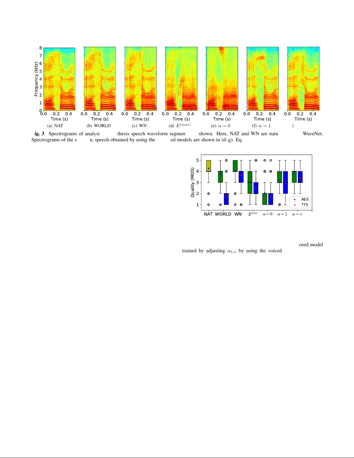
STFT SPECTRAL LOSS FOR TRAINING A NEURAL SPEECH W A VEFORM MODEL Shinji T akaki 1 , T oru Nakashika 2 , Xin W ang 1 , J unichi Y amagishi 1 , 3 1 National Institute of Informatics, Japan 2 The Uni versity of Electro-Communications, Japan 3 The Uni versity of Edinb urgh, UK takaki@nii.ac.jp, nakashika@uec.ac.jp, wangxin@nii.ac.jp, jyamagis@nii.ac.jp ABSTRA CT This paper proposes a new loss using short-time Fourier transform (STFT) spectra for the aim of training a high-performance neural speech wa veform model that predicts raw continuous speech wa ve- form samples directly . Not only amplitude spectra but also phase spectra obtained from generated speech wav eforms are used to cal- culate the proposed loss. W e also mathematically sho w that training of the wa veform model on the basis of the proposed loss can be inter- preted as maximum likelihood training that assumes the amplitude and phase spectra of generated speech wav eforms follo wing Gaus- sian and von Mises distributions, respectiv ely . Furthermore, this paper presents a simple network architecture as the speech wa ve- form model, which is composed of uni-directional long short-term memories (LSTMs) and an auto-regressi ve structure. Experimen- tal results sho wed that the proposed neural model synthesized high- quality speech wa veforms. Index T erms — speech synthesis, neural wav eform modeling, W av eNet 1. INTR ODUCTION Research on speech waveform modeling is advancing because of neural networks [1, 2]. The W aveNet [2] directly models wav eform signals and demonstrates excellent performance. The W aveNet can also be used as a vocoder , which con verts acoustic features, e.g., a mel-spectrogram sequence, into speech wav eform signals [3, 4]. Such a neural speech wa veform model used as a v ocoder can be inte- grated into a text-to-speech synthesis system, and it has been shown that it outperforms conv entional signal-processing-based vocoders [5]. Neural speech waveform models will be essential components for many speech synthesis applications. There hav e been several investig ations of neural speech wave- form models about output distribution and training criteria. A cat- egorical distribution for discrete wa veform samples and cross en- tropy are introduced to train the original W a veNet [2]. The mix- ture of logistic distribution and a discretized logistic mixture likeli- hood are also used to train the improved W a veNet [6]. The parallel- W av eNet [6] and the ClariNet [7] use a distilling approach to trans- fer the knowledge of auto-regressiv e (AR) W av eNet to a simpler non-AR student model. The distilling approach typically introduces an amplitude spectral loss as the auxiliary loss in the distillation in order to a void generating dev oiced/whisper v oices. W e believ e that losses using short-time Fourier transform (STFT) spectra can be This work was partially supported by JST CREST Grant Number JP- MJCR18A6, Japan and by MEXT KAKENHI Grant Numbers (16H06302, 16K16096, 17H04687, 18H04120, 18H04112, 18KT0051, 18K18069), Japan. used beyond the distillation, and they can be used for training speech wa veform models themselves. Because it is known that (complex- valued) STFT spectra represent speech characteristics well, the spec- tra w ould be useful for efficient training of neural wav eform models. In this paper, we propose a new loss using the STFT spectra for the aim of training a high-performance neural speech wav eform model that predicts raw continuous speech waveform samples di- rectly (rather than the auxiliary loss used for the distillation pro- cess). Because not only amplitude spectra but also phase spectra represent speech characteristics [8], the proposed loss considers both amplitude and phase spectral losses obtained from generated speech wa veforms. Also, we give interpretation based on probability distri- butions about training using the proposed loss. This interpretation provides us better understanding of the proposed method and its re- lationship to v arious spectral losses such as Kullback-Leibler diver - gence or Itakura–Saito div ergence [9, 10]. This paper also presents a simple network architecture as a speech wav eform model. The proposed simple network is composed of uni-directional long short- term memories (LSTMs) and an auto-regressiv e structure unlike the W av eNet, which uses a relatively complicated conv olutional neural network (CNN) with stacked dilated con volution. The rest of this paper is organized as follows. Section 2 of this paper presents a neural speech wav eform and the proposed loss to train it. Section 3 describes the proposed network architecture. Ex- perimental results are presented in Section 4. W e conclude in Section 5 with a summary and mention of our future work. 2. THE PR OPOSED LOSS FOR A W A VEFORM MODEL A neural speech waveform model tar geted in this paper is as follo ws. y = f ( λ ) ( x ) , (1) where, y ∈ R M , x = [ x > 1 , ... x > I ] > , x i ∈ R D , and λ represent a neural network’ s outputs (i.e., speech waveform samples), an input sequence (e.g., a log-mel spectrogram), an input feature, and param- eters of a neural network, respectively . A sample index, a frame index, and the dimension of an input feature are represented by m , i , and D , respectiv ely . Back-propagation is generally used to get op- timal parameters λ for a loss function. Because training the model is a regression task, a simple loss function is a square error between natural speech wav eform samples and a neural network’ s outputs y as follows. E ( wav ) = X m ( ˆ y m − y m ) 2 , (2) where, ˆ · denotes natural data. Howe ver , this criterion does not con- sider any information related to frequency characteristics of speech. y Y = W ( DF T ) W ( DF T ) W ( DF T ) W ( DF T ) Y 1 Y 2 Y 3 Y 4 W L S Fig. 1 . STFT complex spectra calculated by using a matrix W . Here, W ∈ C LT × M represents an STFT operation. L , S , and W ( DF T ) denote frame length, frame shift, and a discrete F ourier transform (DFT) matrix. White parts in the matrix W represent 0 . In this paper, we propose loss functions using STFT spectra to ef- fectiv ely train a neural speech waveform instead of using the above square error as a loss function. 2.1. STFT spectra In this section, we describe representations of amplitude and phase spectra used in the proposed loss. As shown in Fig. 1, an STFT complex spectral sequence, Y = [ Y > 1 , ..., Y > T ] > , is represented by using a matrix W as follows. Y = W y , (3) where, t and W represent a frame index and a matrix which per- forms STFT operation, respecti vely . Also, a complex-v alued, ampli- tude and phase spectra of frequenc y bin n at frame t are represented as follows. Y t,n = W t,n y , (4) A t,n = | Y t,n | = ( y > W H t,n W t,n y ) 1 2 , (5) exp( iθ t,n ) = exp( i ∠ Y t,n ) = Y t,n A t,n = W t,n y ( y > W H t,n W t,n y ) 1 2 , (6) where, A t,n , θ t,n , W t,n , · H , and i represent an amplitude spec- trum, a phase spectrum, a row vector of W , Hermitian transpose, and imaginary unit, respectiv ely . In this paper, Euler’ s formula is applied to a phase spectrum instead of directly using a phase spec- trum. W e use amplitude and phase spectra as shown in Eq. (5) and Eq. (6) for model training. 2.2. Amplitude spectral loss A loss function for an amplitude spectrum of frequency bin n at frame t is defined as a square error . E ( amp ) t,n = 1 2 ( ˆ A t,n − A t,n ) 2 (7) = 1 2 ( ˆ A t,n − ( y > W H t,n W t,n y ) 1 2 ) 2 . (8) W e then obtain a partial deriv ati ve of Eq. (7) w .r .t. y as ∂ E ( amp ) t,n ∂ y =  A t,n − ˆ A t,n  R  exp( iθ t,n ) W H t,n  , (9) where, R ( z ) is a real part of a complex value z . Here the Wirtinger deriv ati ve is used to calculate the partial deriv ativ e in the complex domain. P n ∂ E ( amp ) t,n /∂ y can be efficiently calculated by using an in verse FFT operation. 2.3. Phase spectral loss A phase spectrum is a periodic variable with a period of 2 π . A loss function for a phase spectrum of frequency bin n at frame t is defined as follows to consider this periodic property . E ( ph ) t,n = 1 2    1 − exp( i ( ˆ θ t,n − θ t,n ))    2 (10) = 1 − 1 2 ˆ Y t,n ˆ A t,n ( y > W H t,n W t,n y ) 1 2 W t,n y + ˆ Y t,n ˆ A t,n ( y > W H t,n W t,n y ) 1 2 W t,n y ! , (11) where, · is the complex conjugate. W e obtain a partial deriv ativ e of Eq. (10) w .r .t. y as ∂ E ( ph ) t,n ∂ y = sin( ˆ θ t,n − θ t,n ) I  1 Y t,n W H t,n  , (12) where, I ( z ) denotes an imaginary part of a complex value z . P n ∂ E ( ph ) t,n /∂ y can be also efficiently calculated by using an in- verse FFT operation. 2.4. Loss function for model training A partial deriv ativ e of the amplitude loss function (Eq. (9)) includes a phase spectrum of outputs (i.e., θ t,n ), and that of the phase loss function (Eq. (12)) includes an amplitude spectrum of outputs (i.e., A t,n . Y can be rewritten as A t,n exp( i ( − θ t,n )) ). Thus, the am- plitude and phase losses are related to each other through a neural network’ s outputs during model training, although each loss func- tion focuses on only amplitude or phase spectra. In this paper , a combination of amplitude and phase spectral loss functions is used for training a neural speech wa veform model. E ( sp ) = X t,n ( E ( amp ) t,n + α t,n E ( ph ) t,n ) , (13) where, α t,n denotes a weight parameter . W e use three types of α t,n for training a neural speech wa veform model. α t,n = 0 : Using only the amplitude spectral loss function for model training. α t,n = 1 : Using a simple combination of the amplitude and phase spectral loss functions. α t,n = v t : Here, v t represents a voiced/un voiced flag (1:voiced, 0:un voiced). In this case, we assume that phase spectra in unv oiced parts are random v alues, and hence the phase spectral loss computed in un voiced parts is omitted from model training. 2.5. Interpr etation based on probability distributions First, Eq. (7) and Eq. (10) can be rewritten as follo ws. E ( amp ) t,n = log P g ( ˆ A t,n | ˆ A t,n , 1) − log P g ( ˆ A t,n | A t,n , 1) (14) E ( ph ) t,n = 1 − cos( ˆ θ t,n − θ t,n ) = log P vm ( ˆ θ t,n | ˆ θ t,n , 1) − log P vm ( ˆ θ t,n | θ t,n , 1) , (15) Inp ut ne t Dupl ication Clock rate: 200 Hz (frame shift = 5 ms ) Clock rate: 16 kHz Outp ut ne t Removin g amplitude x y m y ′ m − 1 − τ : m − 1 x ′ m y m − 1 − τ : m − 1 x ′ Fig. 2 . Overvie w of the proposed network. where, P g ( · ) and P vm ( · ) are probability density functions of the Gaussian distribution and the v on Mises distribution. P g ( x | µ, σ 2 ) = 1 √ 2 π σ 2 exp  − ( x − µ ) 2 2 σ 2  (16) P vm ( x | µ, β ) = exp( β cos( x − µ )) 2 π I 0 ( β ) (17) I 0 ( β ) is the modified Bessel function of the first kind of order 0 . From relationships of Eqs. (7), (10), (14), and (15), minimiza- tion of Eq. (13) is equiv alent to that of the log negati ve likelihood L below . L = − log Y t,n P g ( ˆ A t,n | A t,n , 1) P α t,n vm ( ˆ θ t,n | θ t,n , 1) . (18) In other words, the amplitude and phase spectra of a neural network’ s outputs represent mean parameters of the Gaussian distribution and the von Mises distribution, respectiv ely . Thus, optimizing a neural network on the basis of the proposed loss function is the maximum likelihood estimation that uses the above probabilistic functions for the speech wa veform model. In this initial inv estigation we used the Gaussian distribution and the v on Mises distribution to define loss functions for amplitude and phase spectra. But we can easily define other meaningful spectral losses by replacing the distributions with other distrib utions. For in- stance, if we use Poisson or e xponential distribution instead of Gaus- sian distribution, we can define the Kullback-Leibler div ergence or Itakura–Saito di vergence as an amplitude spectral loss [9, 10]. Also, we can easily define a different loss function for phase spectra by replacing the von Mises distribution with other distributions such as the generalized cardioid distrib ution [11], the generalized version of the von Mises distrib ution. 3. NETWORK ARCHITECTURE Fig. 2 shows an overvie w of the proposed network. The processing below the dotted line in Fig. 2 is the same as that used in the W av eNet vocoder [12], in which input features are conv erted to hidden repre- sentations through an input network, and then they are duplicated to adjust time resolution. The processing above the dotted line is con- ceptually the same as that used in the W aveNet vocoder , in which feedback samples and hidden representations are fed back into an output network with an auto-regressiv e structure to output the next speech wav eform sample. Ho wev er, the following are two remark- able differences of the proposed netw ork 1 . 1: An output network is simply based on uni-directional LSTMs. CNNs with stacked dilated con volution are not used in our method. 2: Spectral amplitude information is removed from feedback wa ve- form samples. The output network with an auto-regressiv e structure feeds natural wav eform samples back to the netw ork during teacher - forced training [14]. A netw ork composed of uni-directional LSTMs 1 W e also in vestigated a further improv ed network without the auto- regressi ve structure in order to significantly reduce the computational cost at the synthesis phase. See our next paper [13]. tends to rely on the feedback waveform samples while ignoring the input features if natural waveform samples are directly fed into it. T o solve this problem, feedback wa veform samples are con verted as follows. y 0 m − 1 − τ : m − 1 = F − 1  F ( y m − 1 − τ : m − 1 ) |F ( y m − 1 − τ : m − 1 ) |  , (19) where, F , F − 1 , the fraction bar, and | · | denote FFT operation, in verse FFT operation, element-wise division, and the element-wise absolute, respectively . Speech waveform samples, whose amplitude spectra are 1 , are obtained through the con version. This conv ersion can be regarded as data dropout [15], although amplitude spectra are dropped and are replaced with 1 instead of 0 . 4. EXPERIMENT 4.1. Experimental conditions The proposed neural speech wa veform models were ev aluated as a vocoder 2 . W e used a female speaker (slt) from the CMU-ARCTIC database [16]. 1 , 032 and 50 utterances were used as training and test sets, respectively . Their speech wav eforms have a sampling fre- quency of 16 kHz and a 16-bit PCM format. As an input feature, an 80-dim log-mel spectrogram was used. Frame shift, frame length, and FFT size were 80 , 400 , and 512 , re- spectiv ely . Log-mel spectrograms and wav eform samples were nor- malized to have 0 mean and 1 variance for training the proposed speech wa veform model. Input features, i.e., the log-mel spectrogram sequence, were first con verted into hidden representations through an input network com- posed of an 80 -unit bi-directional LSTM and a CNN with 80 fil- ters whose size is 5 (time direction) × 80 (frequency direction). Then, hidden representations were duplicated to adjust time resolu- tion. The pre vious 400 samples and hidden representations obtained from the input network were fed into an output netw ork. The output network was composed of three 256 -unit Uni-directional LSTMs. Frame shift, frame length, and FFT size used to obtain the STFT spectra of a neural network’ s outputs were 1 , 400 , and 512 , respec- tiv ely . Mini-batches were created, each from 120 randomly selected speech segments. Each mini-batch contained a total of 15 s speech wa veform samples (each speech segment equaled 0.125 s). W e used the Adam optimizer [17], and the number of updating iteration was 100 k. W e trained four speech wa veform models with the proposed net- work architecture. The difference among these four models was the loss function used for model training. Eq. (2) and Eq. (13) with three types of α t,n were used as loss functions for training the four models. For comparison, the W aveNet was trained by using 80 -dim log-mel spectrograms and 1,024 mu-law discrete wav eform samples as input and output training data. The network architecture of the W av eNet was the same as that used in [12]. The WORLD [18] was also used as a baseline signal-processing-based vocoder . Spectral en velopes and aperiodicity measurements obtained by utilizing the WORLD were con verted to 59-dim mel-cepstrum and 21-dim band aperiodicity . The total dimensions of a WORLD acoustic feature was 82 ( 60 (mel-cepstrum) + 1 (voiced/un voiced flag) + 1 (lf0) + 21 (band aperiodicity)). In total, we used six v ocoders (the four pro- posed models, the W av eNet, the WORLD) in the experiment. 2 Synthetic speech samples and codes for model training can be found at https://nii- yamagishilab.github.io/TSNetVocoder/ index.html and https://github.com/nii- yamagishilab/ TSNetVocoder , respectiv ely . 0.0 0.2 0.4 Time (s) 0 1 2 3 4 5 6 7 8 Frequency (kHz) (a) N A T 0.0 0.2 0.4 Time (s) 0 1 2 3 4 5 6 7 8 (b) WORLD 0.0 0.2 0.4 Time (s) 0 1 2 3 4 5 6 7 8 (c) WN 0.0 0.2 0.4 Time (s) 0 1 2 3 4 5 6 7 8 (d) E ( wav ) 0.0 0.2 0.4 Time (s) 0 1 2 3 4 5 6 7 8 (e) α = 0 0.0 0.2 0.4 Time (s) 0 1 2 3 4 5 6 7 8 (f) α = 1 0.0 0.2 0.4 Time (s) 0 1 2 3 4 5 6 7 8 (g) α = v Fig. 3 . Spectrograms of analysis-by-synthesis speech waveform segments are sho wn. Here, N A T and WN are natural and the W av eNet. Spectrograms of the synthetic speech obtained by using the proposed models are shown in (d–g). Eq. (2) and Eq. (13) with three types of α are used as loss functions for model training, respectiv ely . W e ev aluated analysis-by-synthesis (AbS) systems and text-to- speech (TTS) synthesis systems based on the six vocoders. For TTS synthesis systems, acoustic models that con vert linguistic fea- tures to acoustic features (i.e., 80 -dim log-mel spectrogram or 82 - dim WORLD acoustic features) were separately trained. Deep auto- regressi ve (DAR) models [15] were used as acoustic models. From the TTS experimental results, we can see the robustness of the pro- posed waveform model against the degraded input features generated by the acoustic models. 4.2. Experimental results 4.2.1. Spectr ogram Fig. 3 shows spectrograms of analysis-by-synthesis speech wav e- form segments. There is an unv oiced part around 0.2 seconds. W e can see from Fig. 3 (d) and (e) that the proposed models trained by using E ( wav ) and E ( sp ) without the phase spectral loss func- tion (i.e., α = 0 ) generated noisy spectrograms. Also, it can be seen from Fig. 3 (f) that large value amplitude spectra are observed around 7 kHz in the unv oiced part, whereas they are not observed in the natural spectrogram. Such artifacts are not observed in the spectrogram sho wn as Fig. 3 (g). These results indicate that train- ing a proposed model by using the amplitude and phase spectral loss functions is adequate and adjusting the weight parameter α by using the voiced/un voiced flag further improv es the performance. Both spectrograms of the W aveNet and the proposed model trained by adjusting α t,n by using the voiced/un voiced flags (i.e., Fig. 3 (c) and (g)) are similar to the natural one, although the detailed spectral structures are changed. 4.2.2. Subjective evaluation result The subjective ev aluation was conducted using 158 crowd-sourced listeners. Natural samples and samples synthesized from the 12 sys- tems were ev aluated. The number of synthetic samples was 650 ( 13 systems × 50 test sentences). Participants ev aluated speech natural- ness on a fiv e-point mean opinion score (MOS) scale. Each synthetic sample was ev aluated 40 times, giving a total of 26 , 000 data points. Thanks to the large number of data points, dif ferences between all combinations of ev aluated systems are statistically significant (i.e., p < 0 . 05 ). First, among the proposed models, those trained together with the phase spectral loss outperformed the others. Using not only amplitude spectra but also phase spectra to calculate loss is useful NAT WORLD WN E w a v α = 0 α = 1 α = v 1 2 3 4 5 Quality (MOS) AbS TTS Fig. 4 . Box plots on naturalness ev aluation results. Blue and red dots represent the mean results of analysis-by-synthesis and text-to- speech synthesis systems, respectiv ely . for training a neural speech wa veform model. The proposed model trained by adjusting α t,n by using the voiced/un voiced flags ob- tained the best score among the proposed models. Second, it can be seen from Fig. 4 that the best performance of the proposed model (i.e., α = v ) is better than that of the WORLD. In the WORLD, the TTS result is drastically decreased from the AbS result. On the other hand, we can see that the proposed model with the best configuration (i.e., α = v ) is robust against acoustic features predicted from the acoustic model. Finally , compared with the W av eNet, the best performance of the proposed models (i.e., α = v ) is slightly worse. But note that the number of parameters of the proposed model (1.8M) is less than that of the W aveNet (2.3M). Although we need to improv e loss functions and network architecture to achieve comparable performance with the W aveNet, it is obvious that the proposed model achiev ed high- performance speech wa veform modeling. 5. CONCLUSION W e proposed a new STFT spectral loss to train a high-performance speech wa veform model directly . W e also presented a simple network architecture for the model, which is composed of uni- directional LSTMs and an auto-regressiv e structure. Experimental results showed that the proposed model can synthesize high-quality speech wa veforms. This is a part of our sequential work. In our next paper [13], we will show that the above model can be improv ed further to achieve performance comparable with the W aveNet. Our other future work includes training based on other time-frequency analysis such as modified discrete cosine transform. 6. REFERENCES [1] Shinji T akaki, Hirokazu Kameoka, and Junichi Y amagishi, “Direct modeling of frequency spectra and wa veform gener - ation based on phase recovery for DNN-based speech synthe- sis, ” in Pr oc. Interspeech , 2017, pp. 1128–1132. [2] A ¨ aron van den Oord, Sander Dieleman, Heiga Zen, Karen Si- monyan, Oriol V inyals, Ale x Graves, Nal Kalchbrenner, An- drew W . Senior , and K oray Kavukcuoglu, “W av enet: A gener- ativ e model for raw audio, ” CoRR , v ol. abs/1609.03499, 2016. [3] Akira T amamori, T omoki Hayashi, Kazuhiro Kobayashi, Kazuya T akeda, and T omoki T oda, “Speaker -dependent W av eNet vocoder , ” in Pr oc. Interspeech , 2017, pp. 1118–1122. [4] Jonathan Shen, Ruoming Pang, Ron J W eiss, Mike Schuster , Navdeep Jaitly , Zongheng Y ang, Zhifeng Chen, Y u Zhang, Y uxuan W ang, Rj Skerrv-Ryan, et al., “Natural TTS synthe- sis by conditioning W aveNet on Mel spectrogram predictions, ” in Pr oc. ICASSP , 2018, pp. 4779–4783. [5] Xin W ang, Jaime Lorenzo-T rueba, Shinji T akaki, Lauri Juvela, and Junichi Y amagishi, “ A comparison of recent wav eform generation and acoustic modeling methods for neural-netw ork- based speech synthesis, ” in Pr oc. ICASSP , 2018, pp. 4804– 4808. [6] Aaron van den Oord, Y azhe Li, Igor Babuschkin, Karen Si- monyan, Oriol V inyals, K oray Kavukcuoglu, George v an den Driessche, Edward Lockhart, Luis C Cobo, Florian Stimberg, et al., “Parallel W av eNet: Fast high-fidelity speech synthesis, ” arXiv preprint arXiv:1711.10433 , 2017. [7] W ei Ping, Kainan Peng, and Jitong Chen, “Clarinet: Parallel wa ve generation in end-to-end text-to-speech, ” arXiv preprint arXiv:1807.07281 , 2018. [8] Pejman Mowlaee, Rahim Saeidi, and Y annis Stylianou, “IN- TERSPEECH 2014 special session: Phase importance in speech processing applications, ” Interspeech , pp. 1623–1627, 2014. [9] Daniel D Lee and H Sebastian Seung, “ Algorithms for non- negati ve matrix factorization, ” in Proc. NIPS , 2001, pp. 556– 562. [10] P . Smaragdis, B. Raj, and M. Shashanka, “Supervised and semi-supervised separation of sounds from single-channel mixtures, ” Pr oceedings of 7th Int. Conf. Ind. Compon. Anal. Signal Separat. , pp. 414–421, 2007. [11] M. C. Jones and Arthur Pewsey , “ A family of symmetric dis- tributions on the circle, ” Journal of the American Statistical Association , vol. 100, no. 472, pp. 1422–1428, 2005. [12] Jaime Lorenzo-Trueba, Fuming Fang, Xin W ang, Isao Echizen, Junichi Y amagishi, and T omi Kinnunen, “Can we steal your vocal identity from the internet?: Initial in vestigation of cloning obamas voice using gan, wav enet and low-quality found data, ” in Pr oc. Odyssey 2018 The Speaker and Language Recognition W orkshop , 2018, pp. 240–247. [13] Xin W ang, Shinji T akaki, and Junichi Y amagishi, “Neural source-filter-based wav eform model for statistical parametric speech synthesis, ” Submitted to ICASSP 2019 , 2019. [14] Ronald J W illiams and Da vid Zipser, “ A learning algorithm for continually running fully recurrent neural networks, ” Neural computation , vol. 1, no. 2, pp. 270–280, 1989. [15] Xin W ang, Shinji T akaki, and Junichi Y amagishi, “ Autore- gressiv e neural f0 model for statistical parametric speech syn- thesis, ” IEEE/A CM T ransactions on Audio, Speech, and Lan- guage Processing , v ol. 26, no. 8, pp. 1406–1419, 2018. [16] J. K ominek and A. W . Black, “The CMU arctic speech databases, ” F ifth ISCA W orkshop on Speech Synthesis , 2004. [17] Diederik P . Kingma and Jimmy Ba, “ Adam: A method for stochastic optimization, ” CoRR , v ol. abs/1412.6980, 2014. [18] Masanori Morise, Fumiya Y okomori, and Kenji Ozawa, “WORLD: A vocoder-based high-quality speech synthesis sys- tem for real-time applications, ” IEICE T rans. on Information and Systems , vol. 99, no. 7, pp. 1877–1884, 2016. A. DET AILS OF THE P AR TIAL DERIV A TIVES The W irtinger deriv ativ e is used to calculate the partial deriv ativ e with respect to a complex value z in the complex domain as, dE dz = 1 2  ∂ E ∂ R ( z ) − i ∂ E ∂ I ( z )  , (20) dE dz = 1 2  ∂ E ∂ R ( z ) + i ∂ E ∂ I ( z )  . (21) If E is a real function, the complex gradient vector is gi ven by ∇ E = 2 dE d z (22) = ∂ E ∂ R ( z ) + i ∂ E ∂ I ( z ) . (23) For a non-analytic function, the chain rule is gi ven by ∂ E ∂ x = ∂ E ∂ u ∂ u ∂ x + ∂ E ∂ u ∂ u ∂ x . (24) A.1. Derivati ve of amplitude spectral loss E ( amp ) t,n Giv en the amplitude spectral loss E ( amp ) t,n = 1 2 ( ˆ A t,n − A t,n ) 2 . (25) According to the chain rule, we can compute the deriv ati ve ∂ E ( amp ) t,n ∂ y = ( A t,n − ˆ A t,n ) · ∂ A t,n ∂ y . (26) For ∂ A t,n ∂ y , since we know that A t,n = ( y > W H t,n W t,n y ) 1 2 ∈ R , we can compute ∂ A t,n ∂ y = ∂ ( y > W H t,n W t,n y ) 1 2 ∂ y (27) = 1 2 ( y > W H t,n W t,n y ) − 1 2 · ( W H t,n W t,n + W > t,n W t,n ) y (28) = 1 2 ( y > W H t,n W t,n y ) − 1 2 · ( W H t,n W t,n y + W > t,n W t,n y ) (29) = 1 2 ( y > W H t,n W t,n y ) − 1 2 · 2 R ( W H t,n W t,n y ) (30) = 1 A t,n · R ( Y t,n W H t,n ) (31) = R ( Y t,n A t,n W H t,n ) (32) = R (exp( iθ t,n ) W H t,n ) (33) where, · > and · H denotes transpose and Hermititian transpose, respectively . Note that, from Eq. (27) to (28), because W t,n is a complex- valued v ector , we need to use ∂ y > W H t,n W t,n y ∂ y = ( W H t,n W t,n + W > t,n W t,n ) y . (34) From Eqs. (29) to (30), we use the fact that W H t,n W t,n y = W > t,n W t,n y and therefore W H t,n W t,n y + W > t,n W t,n y = 2 R ( W H t,n W t,n y ) . (35) Based on Equation 33 and 26, we finally get ∂ E ( amp ) t,n ∂ y = ( A t,n − ˆ A t,n ) R (exp( iθ t,n ) W H t,n )) . (36) A.2. Derivati ve of phase spectrum loss E ( ph ) t,n Based on the definition of E ( ph ) t,n , we get E ( ph ) t,n = 1 2    1 − exp( i ( ˆ θ t,n − θ t,n ))    2 (37) = 1 2     1 − exp( i ( ˆ θ t,n )) 1 exp( i ( θ t,n ))     2 (38) = 1 2      1 − ˆ Y t,n ˆ A t,n A t,n Y t,n      2 (39) = 1 2 1 − ˆ Y t,n ˆ A t,n A t,n Y t,n ! 1 − ˆ Y t,n ˆ A t,n A t,n Y t,n ! (40) = 1 2 1 − ˆ Y t,n ˆ A t,n A t,n Y t,n ! 1 − ˆ Y t,n ˆ A t,n A t,n Y t,n ! (41) = 1 2 1 + ˆ Y t,n ˆ A t,n A t,n Y t,n ˆ Y t,n ˆ A t,n A t,n Y t,n − ˆ Y t,n ˆ A t,n A t,n Y t,n + ˆ Y t,n ˆ A t,n A t,n Y t,n !! (42) = 1 2 1 + 1 − ˆ Y t,n ˆ A t,n A t,n Y t,n + ˆ Y t,n ˆ A t,n A t,n Y t,n !! (43) = 1 − 1 2 ˆ Y t,n ˆ A t,n A t,n Y t,n + ˆ Y t,n ˆ A t,n A t,n Y t,n ! (44) = 1 − 1 2 1 ˆ A t,n A t,n  ˆ Y Y + ˆ Y Y  . (45) Note that ˆ A t,n , A t,n and ˆ Y Y + ˆ Y Y ∈ R while ˆ Y t,n and Y t,n ∈ C . Also note that Y t,n Y t,n = A 2 t,n and ˆ Y t,n ˆ Y t,n = ˆ A 2 t,n . Thus, we can calculate ∂ E ( ph ) t,n ∂ y as follows. ∂ E ( ph ) t,n ∂ y = 1 2 ∂ ˆ A − 1 t,n A − 1 t,n ∂ y  ˆ Y t,n Y t,n + ˆ Y t,n Y t,n  + 1 ˆ A t,n A t,n ∂ ˆ Y t,n Y t,n + ˆ Y t,n Y t,n ∂ y ! (46) = 1 2 − 1 2 ˆ A t,n A 3 t,n  Y t,n W H t,n + Y t,n W > t,n   ˆ Y t,n Y t,n + ˆ Y t,n Y t,n  + 1 ˆ A t,n A t,n  ˆ Y t,n W > t,n + ˆ Y t,n W H t,n  ! (47) = 1 2 − 1 2 ˆ A t,n A 3 t,n  ˆ Y t,n Y 2 t,n W H t,n + ˆ Y t,n A 2 t,n W H t,n + ˆ Y t,n A 2 t,n W > t,n + ˆ Y t,n Y 2 t,n W > t,n  + 1 ˆ A t,n A t,n  ˆ Y t,n W > t,n + ˆ Y t,n W H t,n  ! (48) = 1 2 − 1 2 ˆ A t,n A t,n  ˆ Y t,n Y t,n Y t,n W H t,n + ˆ Y t,n W H t,n + ˆ Y t,n W > t,n + ˆ Y t,n Y t,n Y t,n W > t,n  + 1 ˆ A t,n A t,n  ˆ Y t,n W > t,n + ˆ Y t,n W H t,n  ! (49) = 1 2 1 2 ˆ A t,n A t,n  ˆ Y t,n W H t,n − ˆ Y t,n Y t,n Y t,n W > t,n + ˆ Y t,n W > t,n − ˆ Y t,n Y t,n Y t,n W H t,n  ! (50) = 1 4 ˆ Y t,n ˆ A t,n Y t,n A t,n  1 Y t,n W H t,n − 1 Y t,n W > t,n  + ˆ Y t,n ˆ A t,n Y t,n A t,n  1 Y t,n W > t,n − 1 Y t,n W H t,n  ! (51) = 1 4 ˆ Y t,n ˆ A t,n A t,n Y t,n  1 Y t,n W H t,n − 1 Y t,n W > t,n  + ˆ Y t,n ˆ A t,n A t,n Y t,n  1 Y t,n W > t,n − 1 Y t,n W H t,n  ! (52) = 1 2 R ˆ Y t,n ˆ A t,n A t,n Y t,n  1 Y t,n W > t,n − 1 Y t,n W H t,n  ! (53) = I  exp( i ( ∠ ˆ Y t,n − ∠ Y t,n ))  I  1 Y t,n W H t,n  (54) = sin( ∠ ˆ Y t,n − ∠ Y t,n ) I  1 Y t,n W H t,n  . (55)