SING: Symbol-to-Instrument Neural Generator

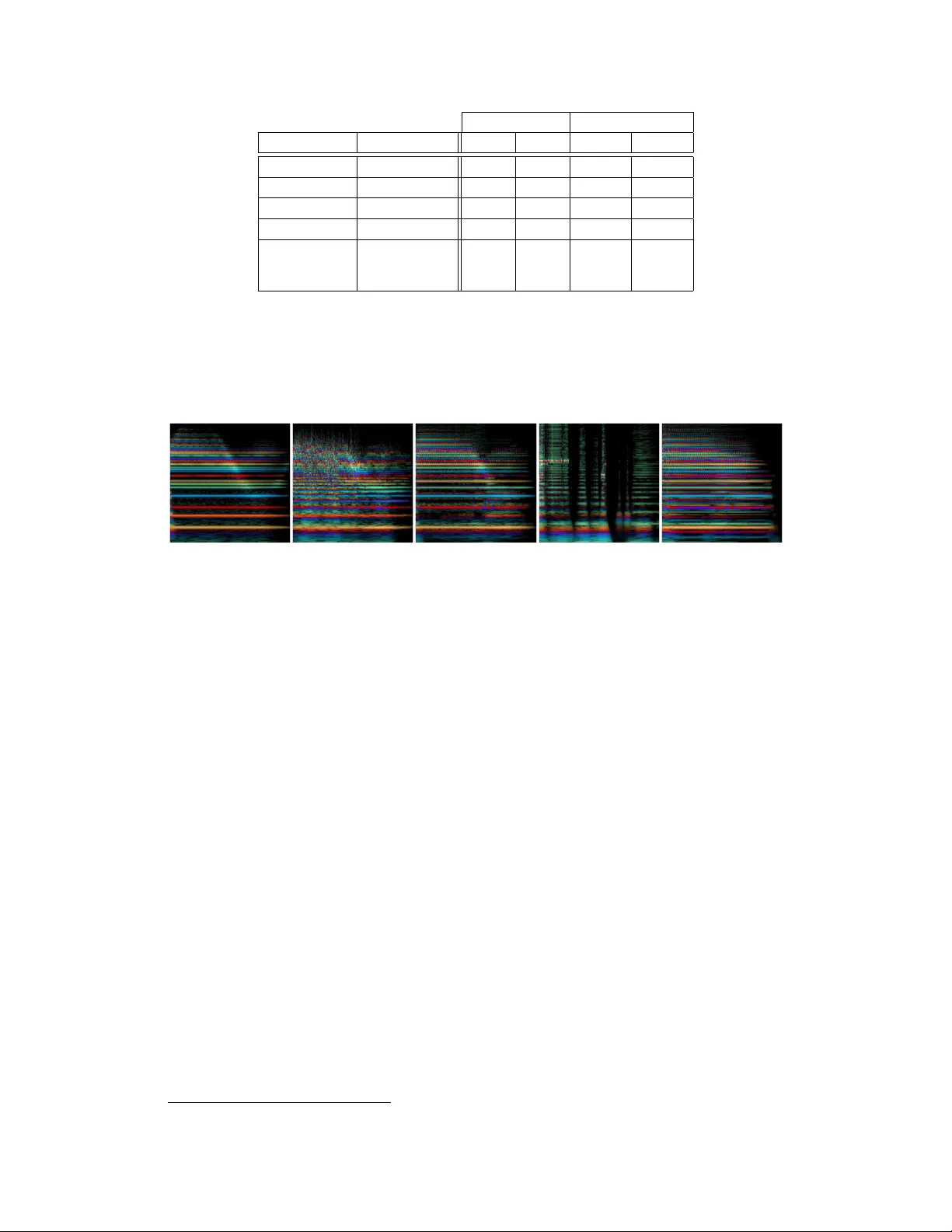
SING: Symbol-to-Instrument Neural Generator Alexandre Déf ossez Facebook AI Research INRIA / ENS PSL Research Univ ersity Paris, France defossez@fb.com Neil Zeghidour Facebook AI Research LSCP / ENS / EHESS / CNRS INRIA / PSL Research Univ ersity Paris, France neilz@fb.com Nicolas Usunier Facebook AI Research Paris, France usunier@fb.com Léon Bottou Facebook AI Research New Y ork, USA leonb@fb.com Francis Bach INRIA École Normale Supérieure PSL Research Univ ersity francis.bach@ens.fr Abstract Recent progress in deep learning for audio synthesis opens the way to models that directly produce the wa veform, shifting away from the traditional paradigm of relying on vocoders or MIDI synthesizers for speech or music generation. Despite their successes, current state-of-the-art neural audio synthesizers such as W av eNet and SampleRNN [ 24 , 17 ] suffer from prohibitiv e training and inference times because they are based on autoregressi ve models that generate audio samples one at a time at a rate of 16kHz. In this work, we study the more computationally efficient alternati ve of generating the wav eform frame-by-frame with large strides. W e present SING, a lightweight neural audio synthesizer for the original task of generating musical notes gi ven desired instrument, pitch and velocity . Our model is trained end-to-end to generate notes from nearly 1000 instruments with a single decoder , thanks to a ne w loss function that minimizes the distances between the log spectrograms of the generated and target wa veforms. On the generalization task of synthesizing notes for pairs of pitch and instrument not seen during training, SING produces audio with significantly improv ed perceptual quality compared to a state-of-the-art autoencoder based on W a veNet [ 4 ] as measured by a Mean Opinion Score (MOS), and is about 32 times faster for training and 2 , 500 times faster for inference. 1 Introduction The recent progress in deep learning for sequence generation has led to the emergence of audio synthesis systems that directly generate the waveform, reaching state-of-the-art perceptual quality in speech synthesis, and promising results for music generation. This represents a shift of paradigm with respect to approaches that generate sequences of parameters to v ocoders in text-to-speech systems [ 21 , 23 , 19 ], or MIDI partition in music generation [ 8 , 3 , 10 ]. A commonality between the state-of- the-art neural audio synthesis models is the use of discretized sample values, so that an audio sample is predicted by a cate gorical distribution trained with a classification loss [ 24 , 17 , 18 , 14 ]. Another significant commonality is the use of autoregressi ve models that generate samples one-by-one, which leads to prohibiti ve training and inference times [ 24 , 17 ], or requires specialized implementations and low-le vel code optimizations to run in real time [ 14 ]. An exception is parallel W av eNet [ 18 ] which generates a sequence with a fully con volutional network for f aster inference. Howe ver , the parallel 32nd Conference on Neural Information Processing Systems (NIPS 2018), Montréal, Canada. approach is trained to reproduce the output of a standard W av eNet, which means that faster inference comes at the cost of increased training time. In this paper , we study an alternati ve to both the modeling of audio samples as a categorical distribution and the autoregressi ve approach. W e propose to generate the waveform for entire audio frames of 1024 samples at a time with a large stride, and model audio samples as continuous v alues. W e dev elop and ev aluate this method on the challenging task of generating musical notes based on the desired instrument, pitch, and velocity , using the large-scale NSynth dataset [ 4 ]. W e obtain a lightweight synthesizer of musical notes composed of a 3-layer RNN with LSTM cells [ 12 ] that produces embeddings of audio frames gi ven the desired instrument, pitch, v elocity 1 and time index. These embeddings are decoded by a single four-layer con volutional network to generate notes from nearly 1000 instruments, 65 pitches per instrument on av erage and 5 velocities. The successful end-to-end training of the synthesizer relies on two ingredients: • A new loss function which we call the spectr al loss , which computes the 1 -norm between the log power spectrograms of the wav eform generated by the model and the target wa veform, where the power spectrograms are obtained by the short-time F ourier transform (STFT). Log power spectrograms are interesting both because they are related to human perception [ 6 ], but more importantly because the entire loss is inv ariant to the original phase of the signal, which can be arbitrary without audible differences. • Initialization with a pre-trained autoencoder: a purely conv olutional autoencoder architecture on raw wa veforms is first trained with the spectral loss. The LSTM is then initialized to reproduce the embeddings gi ven by the encoder , using mean squared error . After initialization, the LSTM and the decoder are fine-tuned together , backpropagating through the spectral loss. W e ev aluate our synthesizer on a new task of pitch completion: generating notes for pitches not seen during training. W e perform perceptual experiments with human ev aluators to aggregate a Mean Opinion Score (MOS) that characterizes the naturalness and appealing of the generated sounds. W e also perform ABX tests to measure the relativ e similarity of the synthesizer’ s ability to ef fectiv ely produce a new pitch for a gi ven instrument, see Section 5.3.2. W e use a state-of-the-art autoencoder of musical notes based on W aveNet [ 4 ] as a baseline neural audio synthesis system. Our synthesizer achiev es higher perceptual quality than W avenet-based autoencoder in terms of MOS and similarity to the ground-truth while being about 32 times faster during training and 2 , 500 times for generation. 2 Related W ork A large body of work in machine learning for audio synthesis focuses on generating parameters for vocoders in speech processing [ 21 , 23 , 19 ] or musical instrument synthesizers in automatic music composition [ 8 , 3 , 10 ]. Our goal is to learn the synthesizers for musical instruments, so we focus here on methods that generate sound without calling such synthesizers. A first type of approaches model power spectrograms giv en by the STFT [ 4 , 9 , 25 ], and generate the wa veform through a post-processing that is not part of the training using a phase reconstruction algorithm such as the Grif fin-Lim algorithm [ 7 ]. The adv antage is to focus on a distance between high- lev el representations that is more relev ant perceptually than a regression on the wav eform. Howe ver , using Grif fin-Lim means that the training is not end to end. Indeed the predicted spectrograms may not come from a real signal. In that case, Griffin-Lim performs an orthogonal projection onto the set of valid spectrograms that is not accounted for during training. Notice that our approach with the spectral loss is dif ferent: our models directly predict wav eforms rather than spectrograms and the spectral loss computes log power spectrograms of these predicted w av eforms. The current state-of-the-art in neural audio synthesis is to generate directly the w aveform [ 24 , 17 , 19 ]. Individual audio samples are modeled with a cate gorical distribution trained with a multiclass cross- entropy loss. Quantization of the 16 bit audio is performed (either linear [ 17 ] or with a µ -law companding [ 24 ]) to map to a few hundred bins to improve scalability . The generation is still extremely costly; distillation [ 11 ] to a faster model has been proposed to reduce inference time at the expense of an e ven larger training time [ 18 ]. The recent proposal of [ 14 ] partly solves the issue with 1 Quoting [ 4 ]: "MIDI velocity is similar to v olume control and they ha ve a direct relationship. For physical intuition, higher velocity corresponds to pressing a piano ke y harder ." 2 a small loss in accuracy , but it requires hea vy low-le vel code optimization. In contrast, our approach trains and generate wa veforms comparably f ast with a PyT orch 2 implementation. Our approach is different since we model the wa veform as a continuous signal and use the spectral loss between generated and target wa veforms and model audio frames of 1024 samples, rather than performing classification on individual samples. The spectral loss we introduce is also different from the power loss regularization of [ 18 ], even though both are based on the STFT of the generated and target wa veforms. In [ 18 ], the primary loss is the classification of indi vidual samples, and their power loss is used to equalize the a verage amplitude of frequencies ov er time. Thus the po wer loss cannot be used alone to learn to reconstruct the wa veform. W orks on neural audio synthesis conditioned on symbolic inputs were dev eloped mostly for text- to-speech synthesis [ 24 , 17 , 25 ]. Experiments on generation of musical tracks based on desired properties were described in [ 24 ], but no systematic ev aluation has been published. The model of [ 4 ], which we use as baseline in our experiments on perceptual quality , is an autoencoder of musical notes based on W aveNet [ 24 ] that compresses the signal to generate high-le vel representations that transfer to music classification tasks, b ut contrarily to our synthesizer , it cannot be used to generate wa veforms from desired properties of the instrument, pitch and velocity without some input signal. The minimization by gradient descent of an objecti ve function based on the po wer spectrogram has already been applied to the transformation of a white noise wa veform into a specific sound te xture [ 2 ]. Howe ver , to the best of our knowledge, such objecti ve functions hav e not been used in the context of neural audio synthesis. 3 The spectral loss f or wav eform synthesis Previous work in audio synthesis on the wav eform focused on classification losses [ 17 , 24 , 4 ]. Howe ver , their computational cost needs to be mitigated by quantization, which inherently limits the resolution of the predictions, and ultimately increasing the number of classes is likely necessary to achie ve the optimal accuracy . Our approach directly predicts a single continuous v alue for each audio sample, and computes distances between wa veforms in the domain of po wer spectra to be in variant to the original phase of the signal. As a baseline, we also consider computing distances between wa veforms using plain mean square error (MSE). 3.1 Mean square r egression on the wa vef orm The simplest way of measuring the distance between a reconstructed signal ˆ x and the reference x is to compute the MSE on the wa veform directly , that is taking the Euclidean norm between x and ˆ x , L wa v ( x, ˆ x ) := k x − ˆ x k 2 . (3.1) The MSE is most lik ely not suited as a perceptual distance between wa veforms because it is extremely sensitiv e to a small shift in the signal. Y et, we observed that it was suf ficient to learn an autoencoder and use it as a baseline. 3.2 Spectral loss As an alternativ e to the MSE on the wav eform, we suggest taking the Short T erm Fourier T ransform (STFT) of both x and ˆ x and compare their absolute values in log scale. W e first compute the log spectrogram l ( x ) := log   + | STFT [ x ] | 2  . (3.2) The STFT decomposes the original signal x in successiv e frames of 1024 time steps with a stride of 256 so that a frame o verlaps at 75% with the ne xt one. The output for a single frame is gi ven by 513 complex numbers, each representing a specific frequenc y range. T aking the point-wise absolute values of those numbers represents how much ener gy is present in a specific frequency range. W e observed that our models generated higher quality sounds when trained using a log scale of those coefficients. Previous work has come to the same conclusion [ 4 ]. W e observed that many entries 2 https://pytorch.org/ 3 of the spectrograms are close to zero and that small errors on those parts can add up to form noisy artifacts. In order to fav or sparsity in the spectrogram, we use the k·k 1 norm instead of the MSE, L stft , 1 ( x, ˆ x ) := k l ( x ) − l ( ˆ x ) k 1 . (3.3) The value of  controls the trade-off between accurately representing low energy and high energy coefficients in the spectrogram. W e found that  = 1 ga ve the best subjecti ve reconstruction quality . The STFT is a (complex) conv olution operator on the wav eform and the squared absolute value of the Fourier coefficients makes the power spectrum differentiable with respect to the generated wa veform. Since the generated wa veform is itself a differentiable function of the parameters (up to the non-dif ferentiability points of activ ation functions such as ReLU), the spectral loss (3.3) can be minimized by standard backpropagation. Even though we only consider this spectral loss in our experiments, alternati ves to the STFT such as the W avelet transform also define differentiable loss for suitable wa velets. 3.2.1 Non unicity of the wav eform r epresentation T o illustrate the importance of the spectral loss instead of a wav eform loss, let us no w consider a problem that arises when generating notes in the test set. Let us assume one of the instrument is a pure sinuoide. For a giv en pitch at a frequenc y f , the audio signal is x i = sin(2 π i f 16000 + φ ) . Our perception of the signal is not af fected by the choice of φ ∈ [0 , 2 π [ , and the po wer spectrogram of x is also unaltered. When recording an acoustic instrument, the v alue of φ depends on any number of variables characterizing the physical system that generated the sound and there is no guarantee that φ stays constant when playing the same note again. For a synthetic sound, φ also depends on implementation details of the software generating the sound. For a sound that is not in the training set and as far as the model is concerned, φ is a random variable that can take any v alue in the range [0 , 2 π [ . As a result, x 0 is unpredictable in the range [ − 1 , 1] , and the mean square error between the generated signal and the ground truth is uninformati ve. Even on the training dataset, the model has to use extra resources to remember the value of φ for each pitch. W e belie ve that this phenomenon is the reason why training the synthesizer using the MSE on the wa veform leads to worse reconstruction performance, e ven though this loss is sufficient in the context of auto-encoding (see Section 5.2). The spectral loss solves this issue since the model is free to choose a single canonical value for φ . Howe ver , one should note that the spectral loss is permissiv e, in the sense that it does not penalize phase inconsitencies of the complex phase across the different frames of the STFT , which lead to potential artifacts. In practice, we obtain state of the art results (see Section 5) and we conjecture that thanks to the frame o verlap in the STFT , the solution that minimizes the spectral loss will often be phase consistent, which is why Griffin-Lim works resonably well despite sharing the same limitation. 4 Model In this section we introduce the SING architecture. It is composed of two parts: a LSTM based sequence generator whose output is plugged to a decoder that transforms it into a wa veform. The model is trained to reco ver a w aveform x sampled at 16,000 Hz from the training set based on the one-hot encoded instrument I , pitch P and velocity V . The whole architecture is summarized in Figure 1. 4.1 LSTM sequence generator The sequence generator is composed of a 3-layer recurrent neural network with LSTM cells and 1024 hidden units each. Given an example with velocity V , instrument I and pitch P , we obtain 3 embeddings ( u V , v I , w P ) ∈ R 2 × R 16 × R 8 from look-up tables that are trained along with the model. Furthermore, the model is provided at each time step with an extra embedding z T ∈ R 4 where T is the current time step [ 22 , 5 ], also obtained from a look-up table that is trained jointly . The input of the LSTM is the concatenation of those four vectors ( u V , v I , w P , z T ) . Although we first experimented with an autore gressiv e model where the previous output was concatenated with those embeddings, we achie ved much better performance and faster training by feeding the LSTM with only on the 4 vectors ( u V , v I , w P , z T ) at each time step. Given those inputs, the recurrent network 4 h 0 := 0 ( u V , v I , w P , z 1 ) s 1 ( V I P ) ( u V , v I , w P , z 2 ) h 1 s 2 ( V I P ) ( u V , v I , w P , z 3 ) h 2 s 3 ( V I P ) · · · ( u V , v I , w P , z 265 ) h 259 s 265 ( V I P ) Conv olution K = 9 , S = 1 , C = 4096 , ReLU Conv olution K = 1 , S = 1 , C = 4096 , ReLU Conv olution K = 1 , S = 1 , C = 4096 , ReLU Conv transpose K = 1024 , S = 256 , C = 1 Output wav eform STFT + log-power Spectral loss Figure 1: Summary of the entire architecture of SING. u V , v I , w P , z ∗ represent the look-up tables respectiv ely for the velocity , instrument, pitch and time. h ∗ represent the hidden state of the LSTM and s ∗ its output. For con volutional layers, K represents the kernel size, S the stride and C the number of channels. generates a sequence ∀ 1 ≤ T ≤ N , s ( V , I , P ) T ∈ R D with a linear layer on top of the last hidden state. In our experiments, we ha ve D = 128 and N = 265 . 4.2 Con volutional decoder The sequence s ( V , I , P ) is decoded into a wa veform by a con volutional network. The first layer is a conv olution with a kernel size of 9 and a stride of 1 over the sequence s with 4096 channels followed by a ReLU. The second and third layers are both con volutions with a kernel size of 1 (a.k.a. 1x1 con volution [ 4 ]) also follo wed by a ReLU. The number of channels is kept at 4096. Finally the last layer is a transposed con volution with a stride of 256 and a kernel size of 1024 that directly outputs the final wav eform corresponding to an audio frame of size 1024 . In order to reduce artifacts generated by the high stride v alue, we smooth the decon volution filters by multiplying them with a squared Hann windo w . As the stride is one fourth of the kernel size, the squared Hann windo w has the property that the sum of its v alues for a gi ven output position is alw ays equal to 1 [ 7 ]. Thus the final decon volution can also be seen as an overlap-add method. W e pad the examples so that the final generated audio signal has the right length. Given our parameters, we need s ( V , I , P ) to be of length N = 265 to recover a 4 seconds signal d ( s ( V , I , P )) ∈ R 64 , 000 . 4.3 T raining details All the models are trained on 4 P100 GPUs using Adam [ 15 ] with a learning rate of 0.0003 and a batch size of 256. Initialization with an autoencoder . W e introduce an encoder turning a w aveform x into a sequence e ( x ) ∈ R N × D . This encoder is almost the mirror of the decoder . It starts with a con volution layer with a kernel size of 1024, a stride of 256 and 4096 channels follo wed by a ReLU. Similarly to the decoder , we smooth its filters using a squared Hann window . Next are two 1x1 conv olutions with 4096 channels and ReLU as an activ ation function. A final 1x1 con volution with no non linearity turns those 4096 channels into the desired sequence with D channels. W e first train the encoder and decoder together as an auto-encoder on a reconstruction task. W e train the auto-encoder for 50 epochs which takes about 12 hours on 4 GPUs. 5 LSTM training. Once the auto-encoder has conv erged, we use the encoder to generate a target sequence for the LSTM. W e use the MSE between the output s ( V , I , P ) of the LSTM and the output e ( x ) of the encoder , only optimizing the LSTM while keeping the encoder constant. The LSTM is trained for 50 epochs using truncated backpropagation through time [ 26 ] using a sequence length of 32. This takes about 10 hours on 4 GPUs. End-to-end fine tuning. W e then plug the decoder on top of the LSTM and fine tune them together in an end-to-end fashion, directly optimizing for the loss on the waveform, either using the MSE on the wa veform or computing the MSE on the log-amplitude spectrograms and back propag ating through the STFT . At that point we stop using truncated back propagation through time and directly compute the gradient on the entire sequence. W e do so for 20 epochs which takes about 8 hours on 4 GPUs. From start to finish, SING takes about 30 hours on 4 GPUs to train. Although we could have initialized our LSTM and decoder randomly and trained end-to-end, we did not achiev e con ver gence until we implemented our initialization strategy . 5 Experiments The source code for SING and a pretrained model are av ailable on our github 3 . Audio samples are av ailable on the article webpage 4 . 5.1 NSynth dataset The train set from the NSynth dataset [ 4 ] is composed of 289,205 audio recordings of instruments, some synthetic and some acoustic. Each recording is 4 second long at 16,000 Hz and is represented by a vector x V ,I ,P ∈ [ − 1 , 1] 64 , 000 index ed by V ∈ { 0 , 4 } representing the velocity of the note, I ∈ { 0 , . . . , 1005 } representing the instrument, P ∈ { 0 , . . . , 120 } representing the pitch. The range of pitches av ailable can vary depending on the instrument b ut for any combination of V , I , P , there is at most a single recording. W e did not make use of the v alidation or test set from the original NSynth dataset because the instruments had no ov erlap with the training set. Because we use a look-up table for the instrument embedding, we cannot generate audio for unseen instruments. Instead, we selected for each instrument 10% of the pitches randomly that we mo ved to a separate test set. Because the pitches are different for each instrument, our model trains on all pitches but not on all combinations of a pitch and an instrument. W e can then ev aluate the ability of our model to generalize to unseen combinations of instrument and pitch. In the rest of the paper , we refer to this ne w split of the original train set as the train and test set. 5.2 Generalization through pitch completion W e report our results in T able 1. W e provided both the performance of the complete model as well as that of the autoencoder used for the initial training of SING. This autoencoder serves as a reference for the maximum quality the model can achiev e if the LSTM were to reconstruct perfectly the sequence e ( x ) . Although using the MSE on the w av eform works well as far as the autoencoder is concerned, this loss is hard to optimize for the LSTM. Indeed, the autoencoder has access to the signal it must reconstruct, so that it can easily choose which repr esentation of the signal to output as explained in Section 3.2.1. SING must be able to recover that information solely from the embeddings giv en to it as input. It manages to learn some of it but there is an important drop in quality . Besides, when switching to the test set one can see that the MSE on the wa veform increases significantly . As the model has ne ver seen those examples, it has no way of picking the right representation. When using a spectral loss, SING is free to choose a canonical representation for the signal it has to reconstruct and it does not hav e to remember the one that was in the training set. W e observe that although we ha ve a drop in quality between the train and test set, our model is still able to generalize to unseen combinations of pitch and instrument. 3 https://github.com/facebookresearch/SING 4 https://research.fb.com/publications/sing- symbol- to- instrument- neural- generator 6 Spectral loss W av MSE Model training loss train test train test Autoencoder wa veform 0.026 0.028 0.0002 0.0003 SING wa veform 0.075 0.084 0.006 0.039 Autoencoder spectral 0.028 0.032 N/A N/A SING spectral 0.039 0.051 N/A N/A SING no time embedding spectral 0.050 0.063 N/A N/A T able 1: Results on the train and test set of the pitch completion task for dif ferent models. The first column specifies the model, either the autoencoder used for the initial training of the LSTM or the complete SING model with the LSTM and the con volutional decoder . W e compare models either trained with a loss on the wa veform (see (3.1) ) or on the spectrograms (see (3.3) ). Finally we also trained a model with no temporal embedding. Figure 2: Example of rainbo wgrams from the NSynth dataset and the reconstructions by different models. Rainbowgrams are defined in [ 4 ] as “a CQT spectrogram with intensity of lines proportional to the log magnitude of the power spectrum and color gi ven by the deriv ativ e of the phase”. Time is represented on the horizontal axis while frequencies are on the vertical one. From left to right: ground truth, W avenet-based autoencoder , SING with spectral loss, SING with wa veform loss and SING without the time embedding. Finally , we tried training a model without the time embedding z T . Theoretically , the LSTM could do without it by learning to count the number of time steps since the beginning of the sequence. Howe ver we do observe a significant drop in performance when removing this embedding, thus motiv ating our choice. On Figure 2, we represented the rainbo wgrams for a particular example from the test set as well as its reconstruction by the W avenet-autoencoder , SING trained with the spectral and wav eform loss and SING without time embedding. Rainbowgrams are defined in [ 4 ] as “a CQT spectrogram with intensity of lines proportional to the log magnitude of the power spectrum and color gi ven by the deriv ative of the phase”. A different deri v ative of the phase will lead to audible deformations of the target signal. Such modification are not penalized by our spectral loss as explained in Section 3.2.1. Nev ertheless, we observe a mostly correct reconstruction of the deri vati ve of the phase using SING. More examples from the test set, including the rainbowgrams and audio files are available on the article webpage 5 . 5.3 Human evaluations During training, we use se veral automatic criteria to ev aluate and select our models. These criteria include the MSE on spectrograms, magnitude spectra, or wa veform, and other perceptually-moti vated metrics such as the Itakura-Saito div ergence [ 13 ]. Howe ver , the correlation of these metrics with human perception remains imperfect, this is why we use human judgments as a metric of comparison between SING and the W avenet baseline from [4]. 5 https://research.fb.com/publications/sing- symbol- to- instrument- neural- generator 7 Model MOS Training time (hrs * GPU) Generation speed Compression factor Model size Ground T ruth 3.86 ± 0.24 - - - - W avenet 2.85 ± 0.24 3840 ∗ 0.2 sec/sec 32 948 MB SING 3.55 ± 0.23 120 512 sec/sec 2133 243 MB T able 2: Mean Opinion Score (MOS) and computational load of the dif ferent models. The training time is expressed in hours * GPU units, the generation time is expressed as the number of seconds of audio that can be generated per second of processing time. The compression factor represents the ratio between the dimensionality of the audio sequences ( 64 , 000 v alues) and either the latent state of W avenet or the input v ectors to SING. W e also report the size of the models, in MB. ( ∗ ) T ime corrected to account for the difference in FLOPs of the GPUs used. 5.3.1 Evaluation of per ceptual quality: Mean Opinion Score The first characteristic that we want to measure from our generated samples is their naturalness: how good they sound to the human ear . T o do so, we perform experiments on Amazon Mechanical T urk [ 1 ] to get a Mean Opinion Score for the ground truth samples, and for the wav eforms generated by SING and the W avenet baseline. W e did not include a Griffin-Lim based baseline as the authors in [4] concluded to the superiority of their W avenet autoencoder . W e randomly select 100 examples from our test set. For the W avenet-autoencoder , we pass these 100 examples through the network and retrie ve the output. The latter is a pre-trained model provided by the authors of [ 4 ] 6 . Notice that all of the 100 samples were used for training of the W avenet- autoencoder , while they were not seen during the training of our models. For SING, we feed it the instrument, pitch and velocity information of each of the 100 samples. W orkers are asked to rate the quality of the samples on a scale from 1 ("V ery annoying and objectionable distortion. T otally silent audio") to 5 ("Imperceptible distortion"). Each of the 300 samples (100 samples per model) is ev aluated by 60 W orkers. The quality of the hardware used by W orkers being variable, this could impede the interpretability of the results. Thus, we use the crowdMOS toolkit [ 20 ] which detects and discards inaccurate scores. This toolkit also allows to only keep the e valuations that are made with headphones (rather than laptop speakers for example), and we choose to do so as good listening conditions are necessary to ensure the v alidity of our measures. W e report the Mean Opinion Score for the ground-truth audio and each of the 2 models in T able 2, along with the 95% confidence interval. W e observe that SING shows a significantly better MOS than the W av enet-autoencoder baseline despite a compression factor which is 66 times higher . Moreover , to spotlight the benefits of our approach compared to the W avenet baseline, we also report three metrics to quantify the computational load of the dif ferent models. The first metric is the training time, e xpressed in hours multiplied by the number of GPUs. The authors of [ 4 ], mention that their model trains for 10 days on 32 GPUs, which amounts to 7680 hours*GPUs. Howe ver , the GPUs used are capable of about half the FLOPs compared to our P100. Therefore, we corrected this v alue to 3840 hours*GPUs. On the other hand, SING is trained in 30 hours on four P100, which is 32 times faster than W avenet. A major drawback of autoregressiv e models such as W avenet is that the generation process is inherently sequential: generating the sample at time t + 1 takes as input the sample at time t . W e timed the generation using the implementation of the W avenet-autoencoder pro vided by the authors, in its fastgen version 7 which is significantly faster than the original model. This yields a 22 minutes time to generate a 4-second sample. On a single P100 GPU, W av enet can generate up to 64 sequences at the same time before reaching the memory limit, which amounts to 0.2 seconds of audio generated per second. On the other hand, SING can generate 512 seconds of audio per second of processing time, and is thus 2500 times faster than W avenet. Finally , SING is also efficient in memory compared to W av enet, as the model size in MB is more than 4 times smaller than the baseline. 5.3.2 ABX similarity measure Besides absolute audio quality of the samples, we also want to ensure that when we condition SING on a chosen combination of instrument, pitch and velocity , we generate a relev ant audio sample. T o 6 https://github.com/tensorflow/magenta/tree/master/magenta/models/ nsynth 7 https://magenta.tensorflow.org/nsynth- fastgen 8 do so, we measure how close samples generated by SING are to the ground-truth relati vely to the W avenet baseline. This measure is made by performing ABX [ 16 ] experiments: the W orker is giv en a ground-truth sample as a reference. Then, they are presented with the corresponding samples of SING and W avenet, in a random order to av oid bias and with the possibility of listening as many times to the samples as necessary . They are asked to pick the sample which is the closest to the reference according to their judgment. W e perform this experiment on 100 ABX triplets made from the same data as for the MOS, each triplet being ev aluated by 10 W orkers. On average o ver 1000 ABX tests, 69 . 7% are in fa vor of SING ov er W av enet, which shows a higher similarity between our generated samples and the target musical notes than W av enet. Conclusion W e introduced a simple model architecture, SING, based on LSTM and conv olutional layers to generate waveforms. W e achieve state-of-the-art results as measured by human ev aluation on the NSynth dataset for a fraction of the training and generation cost of existing methods. W e introduced a spectral loss on the generated w aveform as a way of using time-frequenc y based metrics without requiring a post-processing step to recover the phase of a power spectrogram. W e experimentally validated that SING was able to embed music notes into a small dimension v ector space where the pitch, instrument and velocity were disentangled when trained with this spectral loss, as well as synthesizing pairs of instruments and pitches that were not present in the training set. W e believe SING opens up new opportunities for lightweight quality audio synthesis with potential applications for speech synthesis and music generation. Acknowledgments Authors thank Adam Polyak for his help on setting up the human e valuations and Ax el Roebel for the insightful discussions. W e also thank the Magenta team for their inspiring work on NSynth. 9 References [1] Michael Buhrmester , Trac y Kwang, and Samuel D Gosling. Amazon’ s mechanical turk: A new source of inexpensi ve, yet high-quality , data? P erspectives on psycholo gical science , 6(1):3–5, 2011. [2] Hugo Caracalla and Ax el Roebel. Gradient conv ersion between time and frequency domains using wirtinger calculus. In DAFx 2017 , 2017. [3] Kemal Ebcio ˘ glu. An expert system for harmonizing four-part chorales. Computer Music Journal , 12(3):43–51, 1988. [4] Jesse Engel, Cinjon Resnick, Adam Roberts, Sander Dieleman, Douglas Eck, Karen Simonyan, and Mohammad Norouzi. Neural audio synthesis of musical notes with wav enet autoencoders. T echnical Report 1704.01279, arXiv , 2017. [5] Jonas Gehring, Michael Auli, David Grangier , Denis Y arats, and Y ann N Dauphin. Con volutional sequence to sequence learning. arXiv preprint , 2017. [6] JL Goldstein. Auditory nonlinearity . The Journal of the Acoustical Society of America , 41(3):676–699, 1967. [7] Daniel Grif fin and Jae Lim. Signal estimation from modified short-time fourier transform. IEEE T ransactions on Acoustics, Speech, and Signal Processing , 32(2):236–243, 1984. [8] Gaëtan Hadjeres, François Pachet, and Frank Nielsen. Deepbach: a steerable model for bach chorales generation. T echnical Report 1612.01010, arXiv , 2016. [9] Albert Haque, Michelle Guo, and Prateek V erma. Conditional end-to-end audio transforms. T echnical Report 1804.00047, arXiv , 2018. [10] Dorien Herremans. Morpheus: automatic music generation with recurrent pattern constraints and tension profiles. 2016. [11] Geoffre y Hinton, Oriol V inyals, and Jef f Dean. Distilling the knowledge in a neural netw ork. T echnical Report 1503.02531, arXiv , 2015. [12] Sepp Hochreiter and Jürgen Schmidhuber . Long short-term memory . Neural computation , 9(8):1735–1780, 1997. [13] Fumitada Itakura. Analysis synthesis telephony based on the maximum likelihood method. In The 6th international congr ess on acoustics, 1968 , pages 280–292, 1968. [14] Nal Kalchbrenner , Erich Elsen, Karen Simonyan, Seb Noury , Norman Casagrande, Edward Lockhart, Florian Stimberg, Aaron v an den Oord, Sander Dieleman, and K oray Kavukcuoglu. Efficient neural audio synthesis. T echnical Report 1802.08435, arXi v , 2018. [15] Diederik P Kingma and Jimmy Ba. Adam: A method for stochastic optimization. In Interna- tional Confer ence on Learning Repr esentations , 2015. [16] Neil A Macmillan and C Douglas Creelman. Detection theory: A user’ s guide . Psychology press, 2004. [17] Soroush Mehri, Kundan K umar , Ishaan Gulrajani, Rithesh Kumar , Shubham Jain, Jose Sotelo, Aaron Courville, and Y oshua Bengio. Samplernn: An unconditional end-to-end neural audio generation model. T echnical Report 1612.07837, arXiv , 2016. [18] Aaron van den Oord, Y azhe Li, Igor Babuschkin, Karen Simonyan, Oriol V inyals, Koray Kavukcuoglu, Geor ge van den Driessche, Edward Lockhart, Luis C Cobo, Florian Stimber g, et al. Parallel wa venet: Fast high-fidelity speech synthesis. T echnical Report 1711.10433, arXi v , 2017. [19] W ei Ping, Kainan Peng, Andrew Gibiansky , S Arik, Ajay Kannan, Sharan Narang, Jonathan Raiman, and John Miller . Deep voice 3: Scaling text-to-speech with con volutional sequence learning. In Pr oc. 6th International Conference on Learning Representations , 2018. 10 [20] Flávio Ribeiro, Dinei Florêncio, Cha Zhang, and Michael Seltzer . Crowdmos: An approach for crowdsourcing mean opinion score studies. In Acoustics, Speech and Signal Processing (ICASSP), 2011 IEEE International Confer ence on , pages 2416–2419. IEEE, 2011. [21] Jose Sotelo, Soroush Mehri, K undan Kumar , Joao Felipe Santos, K yle Kastner , Aaron Courville, and Y oshua Bengio. Char2wav: End-to-end speech synthesis. 2017. [22] Sainbayar Sukhbaatar, Jason W eston, Rob Fergus, et al. End-to-end memory networks. In Advances in neural information processing systems , pages 2440–2448, 2015. [23] Y aniv T aigman, Lior W olf, Adam Polyak, and Eliya Nachmani. V oice synthesis for in-the-wild speakers via a phonological loop. T echnical Report 1707.06588, arXiv , 2017. [24] Aaron V an Den Oord, Sander Dieleman, Heiga Zen, Karen Simonyan, Oriol V inyals, Alex Grav es, Nal Kalchbrenner , Andrew Senior , and K oray Kavukcuoglu. W avenet: A generativ e model for raw audio. T echnical Report 1609.03499, arXiv , 2016. [25] Y uxuan W ang, RJ Skerry-Ryan, Daisy Stanton, Y onghui Wu, Ron J W eiss, Navdeep Jaitly , Zongheng Y ang, Y ing Xiao, Zhifeng Chen, Samy Bengio, et al. T acotron: T o wards end-to-end speech synthesis. T echnical Report 1703.10135, arXiv , 2017. [26] Ronald J W illiams and Da vid Zipser . Gradient-based learning algorithms for recurrent networks and their computational complexity . Backpr opagation: Theory , ar chitectur es, and applications , 1:433–486, 1995. 11