On Micromechanical Parameter Identification With Integrated DIC and the Role of Accuracy in Kinematic Boundary Conditions

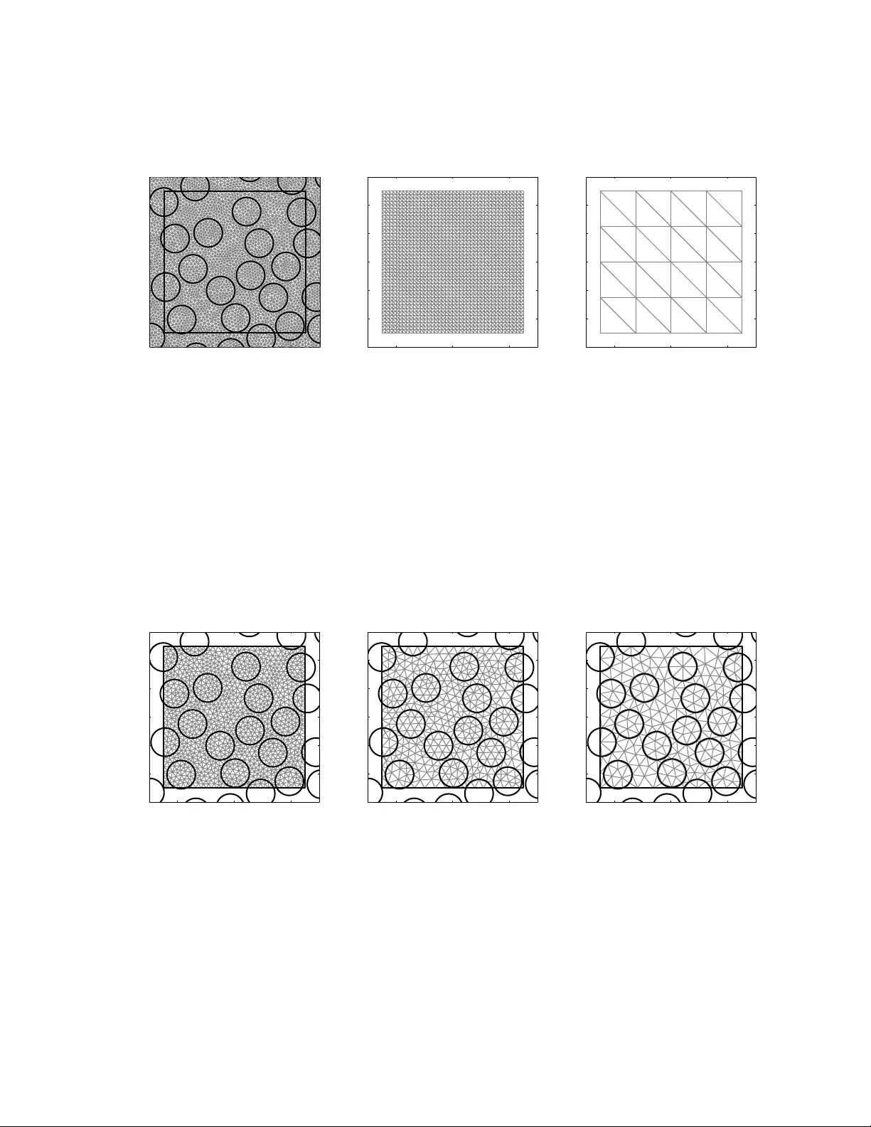
On Micromec hanical P arameter Iden tiﬁcation With In tegrated DIC and the Role of Accuracy in Kinematic Boundary Conditions I O. Rok o ˇ s a, ∗ , J.P .M. Ho efnagels a , R.H.J. P eerlings a , M.G.D. Geers a a Eindhoven University of T e chnolo gy, Dep artment of Me chanic al Engine ering, P.O. Box 513, 5600 MB Eindhoven, The Netherlands Abstract In tegrated Digital Image Correlation (IDIC) is now ada ys a well established full-ﬁeld exp eri- men tal pro cedure for reliable and accurate identiﬁcation of material parameters. It is based on the correlation of a series of images captured during a mec hanical exp eriment, that are matc hed by displacemen t ﬁelds deriv ed from an underlying mechanical mo del. In recent studies, it has b een sho wn that when the applied b oundary conditions lie outside the em- plo yed ﬁeld of view, IDIC suﬀers from inaccuracies. A typical example is a micromechanical parameter iden tiﬁcation inside a Microstructural V olume Elemen t (MVE), whereb y images are usually obtained b y electron microscop y or other microscop y techniques but the loads are applied at a muc h larger scale. F or an y IDIC mo del, MVE b oundary conditions still need to b e sp eciﬁed, and any deviation or ﬂuctuation in these b oundary conditions may signiﬁcan tly inﬂuence the qualit y of identiﬁcation. Prescribing prop er b oundary conditions is generally a c hallenging task, b ecause the MVE has no free b oundary , and the b oundary displacemen ts are typically highly heterogeneous due to the underlying microstructure. The aim of this pap er is therefore ﬁrst to quan tify the eﬀects of errors in the prescrib ed b oundary conditions on the accuracy of the iden tiﬁcation in a systematic wa y . T o this end, three kinds of mechanical tests, each for v arious lev els of material contrast ratios and lev els of image noise, are carried out by means of virtual exp erimen ts. F or simplicity , an elastic compress- ible Neo-Ho okean constitutive mo del under plane strain assumption is adopted. It is sho wn that a high lev el of detail is required in the applied b oundary conditions. This motiv ates an impro ved b oundary condition application approac h, which considers constitutive material parameters as w ell as kinematic v ariables at the b oundary of the entire MVE as degrees of freedom in the IDIC pro cedure, assuring that b oth are iden tiﬁed with equal precision and imp ortance. This problem has b een studied in the literature with a diﬀeren t metho d, i.e. Finite Elemen t Metho d Up dating framework. Keywor ds: In tegrated Digital Image Correlation, parameter identiﬁcation, kinematic b oundary conditions, virtual exp erimen t, micromechanics, inv erse metho ds I The post-print v ersion of this article is published in Int. J. Solids. Struct. , 10.1016/j.ijsolstr.2018.04.004 . ∗ Corresp onding author. Email addr ess: o.rokos@tue.nl (O. Roko ˇ s) Pr eprint submitte d to Int. J. Solids. Struct. Octob er 22, 2018 1. In tro duction Accurate iden tiﬁcation of micromec hanical parameters is imp ortant in n umerous areas of science and engineering. On the one hand, parameters are required for (complex) constitutive la ws that help to predict, e.g., mec hanical resp onse, p erformance, or lifespan of electronic, micro-electro-mec hanical, or other mechanical devices. On the other hand, they help to b etter understand complex ph ysical pro cesses in materials o ccurring across the scales, such as plasticit y , failure, ductile damage, or delamination and crack growth Ho c et al. ( 2003 ); Rupil et al. ( 2011 ); Bla ysat et al. ( 2015 ); Buljac et al. ( 2017 ). Due to their intrinsically small dimensions, micro- or nanoscale mec hanical tests are chal- lenging and necessitate adv anced exp erimental metho ds. One suc h metho d is Digital Image Correlation (DIC), which is a non-in trusiv e full-ﬁeld measuremen t technique with high ac- curacy and reliability that emerged from the recent progress in computer tec hnology and digital imaging. In particular, its in tegrated v arian t called Integrated Digital Image Cor- relation (IDIC) has pro ven to be a reliable and accurate tec hnique for the iden tiﬁcation of material parameters, see e.g. Roux and Hild ( 2006 ); Leclerc et al. ( 2009 ); R´ ethor ´ e et al. ( 2009 , 2013 ); Neggers et al. ( 2015 ); Ruybalid et al. ( 2016 ). It relies on the minimization of the dif- ference b et ween tw o images captured during an exp eriment (corresp onding to the reference and a deformed conﬁguration) inside the Region Of Interest (R OI). The deformed image is bac k-deformed using a displacemen t ﬁeld that is obtained from an underlying mec hani- cal mo del with assumed constitutive la ws and Boundary Conditions (BCs). The required basics of IDIC together with geometry , constitutiv e mo del, and mec hanical tests emplo yed throughout this pap er are sp eciﬁed in more detail in Section 2 . If the BCs applied to a tested specimen lie outside the Field Of View (F OV), IDIC suﬀers from inaccuracies ( Ruybalid et al. , 2017 ). This problem t ypically applies to micromechanical parameter identiﬁcation, see Fig. 1 , whereby images are obtained by electron microscopy or other microscopy tec hniques and the loads are applied at a m uch larger scale. Prescribing prop er b oundary conditions to a giv en Microstructural V olume Elemen t (MVE) is a chal- lenging task, as the MVE has no free boundary , and the displacemen ts along its b oundary are highly heterogeneous due to the presence of microstructural constituents with (highly) con trasting mec hanical b ehavior at or near the b oundary . This renders an y kind of ideal- ized b oundary conditions inappropriate. Several approaches hav e b een prop osed and tested in the literature to resolv e this issue, based on Virtual Fields Metho d (VFM), as reported e.g. in ( Gr ´ ediac et al. , 2006 ; Rahmani et al. , 2014 ), or Finite Elemen t Method Up dat- ing (FEMU) with virtual b oundaries, as prop osed by F edele ( 2015 ). In this contribution, the IDIC metho dology will b e adopted, which has been rep orted e.g. b y Tian et al. ( 2010 ), Hild et al. ( 2016 ), or Shak o or et al. ( 2017 ). According to Shakoor et al. ( 2017 ), so far the most accurate metho dology employs Global Digital Image Correlation (GDIC) in order to iden tify displacemen ts that are subsequently applied as BCs to the MVE asso ciated with IDIC; this approac h will b e referred to as GDIC-IDIC in the sequel. As w ell-known from the literature, cf. e.g. Bornert et al. ( 2009 ); Leclerc et al. ( 2012 ); Hild et al. ( 2016 ), in general (G)DIC on the one hand lacks suﬃcient kinematic freedom when large elemen ts or globally supp orted p olynomials are used (kinematic smo othing), 2 Ω fov X 2 X 1 Ω roi Ω u D − 4 0 − 3 0 − 2 0 − 1 0 0 1 0 2 0 3 0 4 0 − 2 0 − 1 5 − 1 0 − 5 0 5 1 0 1 5 2 0 Figure 1: Sketc h of a t ypical exp erimen tal set-up. Mechanical test carried out on a specimen with a domain Ω, ﬁeld of view Ω fov , and a region of interest Ω roi . while on the other hand it suﬀers from random errors when relatively small elemen ts or lo cally supp orted in terp olation functions are emplo y ed. This indicates a p ossible pitfall for the GDIC-IDIC approac h b ecause, as the BCs are kept ﬁxed during the IDIC parameter iden tiﬁcation pro cedure, any errors in tro duced through the BCs remain lo c ked. The only w ay in which the MVE model can comp ensate for erroneous BCs is by adjusting the material parameters—hence resulting in an inaccurate iden tiﬁcation of these parameters. The ﬁrst aim of this pap er is therefore to systematically quantify the eﬀects of inaccuracies in prescrib ed BCs on the accuracy of the identiﬁcation b y means of virtual exp erimen ts. Some of the obtained results can already be inferred from Fig. 2 , where eﬀects of kinematic smo othing are demonstrated. Without going into many details, ab out whic h the in terested reader is in vited to learn more in Sections 2 and 3 , we note that the iden tiﬁed parameters rapidly deviate from their exact v alue with increasing smo othing k ernel size ε . The exact and smo othed BCs, for the w orst case considered ( ε = 5), are shown in Fig. 2c , indicating that small deviations are at the ro ot of relatively p o or identiﬁcation. This kind of b ehaviour is t ypical and can be explained by extensiv e constrain ts of the MVE system b y Diric hlet BCs applied along the entire b oundary , and by asso ciated sensitivit y ﬁelds of lo w magnitudes, as w e will detail in Section 3 . The second ob jectiv e of this pap er is to provide a metho dology ensuring the desired high accuracy in identifying material parameters and b oundary data. The prop osed approach essen tially incorp orates all Degrees Of F reedom (DOFs) asso ciated with b oundary no des of the MVE mo del as DOFs in the IDIC pro cedure, and will b e referred to as Boundary- Enric hed In tegrated Digital Image Correlation (BE-IDIC) in what follo ws. The metho d signiﬁcan tly impro ves the accuracy of the iden tiﬁed parameters while b eing robust with resp ect to image noise and material contrast ratio. Although this metho dology ma y resem ble the one prop osed b y F edele ( 2015 ), in whic h kinematic BCs are also introduced as DOFs of the micromechanical parameter identiﬁcation routine, important diﬀerences exist. These diﬀerences will b e discussed in detail in Section 4 , along with a detailed description of the BE-IDIC. The pap er ﬁnally closes with a summary and conclusions in Section 5 . 3 λ K 2 /K 2 λ G 2 /G 2 λ G 1 /G 1 λ / λ e x σ 0 0 . 0 5 0 . 1 0 0 . 5 1 1 . 5 2 ε λ/λ ex 0 2 4 0 0 . 5 1 (a) identiﬁed parameter ε λ / λ ex 0 2 4 0 0 . 5 1 (b) identiﬁed parameters smo othed exact ξ u x , u y a b c d a − 0 . 2 0 0 . 2 (c) u ( ∂ Ω mv e ) for ε = 5 Figure 2: An example of iden tiﬁed results for a sheared sp ecimen consisting of randomly distributed stiﬀ inclusions em b edded in a soft matrix, corresponding to 50 Mon te Carlo realizations. Before identiﬁcation, the exact b oundary displacemen ts are smo othed using the pillbox-shaped kernel with a dimensionless (normalized b y inclusion’s size) diameter ε ∈ [0 , 5]; the exact and smo othed displacemen ts are compared in (c). F or iden tiﬁcation, Ω mv e = Ω roi and zero image noise are used. A single parameter identiﬁcation of the matrix shear modulus ( λ = G 1 ) is sho wn in (a); m ultiple parameter iden tiﬁcation of the matrix and inclusion’s shear mo duli together with inclusion’s bulk mo dulus ( λ = [ G 1 , G 2 , K 2 ] T ) are shown in (b). The thick lines corresp ond to the mean v alues whereas shaded areas delimit the standard deviations ov er all realizations. 2. Theory and Problem Statement The basics of DIC, needed for subsequent developmen ts, are ﬁrst recalled in this section. Next, three mechanical tests are described that serve to demonstrate the sensitivit y of the IDIC tec hnology to Diric hlet BCs. In Section 4 , the same mec hanical tests will b e used to assess the BE-IDIC approac h. Next, the constitutive mo del emplo yed throughout this w ork is sp eciﬁed, and sensitivity ﬁelds are shown. Finally , the sp eckle pattern and creation of deformed images are brieﬂy describ ed. 2.1. Digital Image Corr elation In its simplest form, DIC correlates t w o images captured during an exp erimen t, one in the reference conﬁguration and one deformed. These images are in essence scalar ﬁelds supp orted in the F OV, storing usually gra y lev el v alues (e.g. integer num bers ranging [0 , 255] when 8-bit digitization is used). Up on deﬁning a ROI, one aims to ﬁnd a vector λ of n λ IDIC DOFs that minimizes in the least-square sense the diﬀerence b etw een grey v alues in the reference image and in the corresp onding material p oin ts in the deformed image as predicted b y a displacement ﬁeld u , i.e. λ ∈ arg min b λ ∈ R n λ R ( b λ ) , R ( b λ ) = 1 2 Z Ω roi [ f ( X ) − g ( X + u ( X , b λ ))] 2 d X . (1) 4 In ( 1 ), X = [ X 1 , X 2 ] T ∈ R 2 stores the material co ordinates in the reference conﬁguration, and u ( X , b λ ) = [ u 1 ( X , b λ ) , u 2 ( X , b λ )] T is an appro ximate displacemen t ﬁeld that is required in order to regularize the otherwise ill-p osed problem; for more details see e.g. Horn and Sc hunc k ( 1981 ). Throughout this work, the hatted v ariables b • relate to arbitrary admissible v alues, whereas the absence of hats indicates minimizers of the corresp onding cost functional. As indicated by the inclusion sign ∈ , the cost functional R ma y b e non-conv ex with multiple minima; in suc h a case, the global minimum is sought. If the appro ximate ﬁeld u ( X , b λ ) is c hosen such that u ( X , b λ ) = n λ X i =1 ψ i ( X ) b λ i , (2) one recov ers GDIC, where ψ i ( X ) are user-selected vector interpolation (or basis) functions, usually expressed in terms of globally- or lo cally-supp orted polynomials. The v ariable b λ = [ b λ 1 , . . . , b λ n λ ] T ∈ R n λ then constitutes an admissible v ector of generalized displacements. On the con trary , if u ( X , b λ ) ∈ arg min b u ( X , b λ ) ∈ U ( b λ ) E ( b u ( X , b λ ) , b λ ) , (3) is a solution to an underlying (elastic for simplicit y) mec hanical system sp eciﬁed b y its stored energy E and a prop er function space U (see e.g. Ev ans 2010 ), the IDIC metho d results. In practice, a Finite Elemen t (FE) discretization of b u ( X , b λ ) is used (see e.g. Zienkiewicz and T a ylor 2000 ; Ciarlet 2002 ), typically given by b u ( X , b λ ) = n u / 2 X i =1 N i ( X ) b u i ( b λ ) , (4) where b u = [ b u T 1 , . . . , b u T n u / 2 ] T ∈ R n u , b u i = [ b u i 1 , b u i 2 ] T ∈ R 2 , stores displacemen ts of the i -th no de asso ciated with a FE mesh in X 1 and X 2 directions, and N i ( X ) are standard FE shap e functions. In IDIC, b λ can store kinematic v ariables suc h as prescrib ed BCs, or material constan ts—hence the dep endence of U as well as E on b λ . Similarly to the DIC cost func- tional R speciﬁed in Eq. ( 1 ), E ma y b e non-conv ex, allo wing, e.g., for structural buc kling and bifurcation. In order to minimize ( 1 ), v arious approac hes are b eing used. Although w orking only in the proximit y of a lo cal minim um, the most frequen tly emplo yed one is a standard Newton, or more precisely a Gauss-Newton algorithm, that iteratively solv es the following system of linear equations (obtained by a T a ylor expansion of the ﬁrst-order optimalit y conditions in b λ ): H l ( b λ l +1 − b λ l ) = − g l . (5) The individual comp onen ts of the gradien t g and Hessian H , deriv ed b y diﬀeren tiating ( 1 ), 5 read ( g l ) i = ( g ( b λ l )) i = − Z Ω roi ϕ i ( X , b λ ) · ∇ f ( X ) h f ( X ) − g ( X + u ( X , b λ )) i d X     b λ = b λ l , ( H l ) ij = ( H ( b λ l )) ij = Z Ω roi ϕ i ( X , b λ ) · ∇ f ( X ) ∇ f ( X ) · ϕ j ( X , b λ ) d X     b λ = b λ l . (6) Note that ∇ ( • ) = ∂ ( • ) /∂ X , and that a simpliﬁed v ersion of the Hessian is used here, see Neggers et al. ( 2016 ) for further details. In Eqs. ( 6 ), the so-called sensitivit y ﬁelds, deﬁned as ϕ i ( X , b λ ) = ∂ u ( X , b λ ) ∂ b λ i , i = 1 , . . . , n λ , (7) are required. In the case of GDIC, ϕ i ( X ) = ψ i ( X ), i = 1 , . . . , n λ , whereas in the case of IDIC, ϕ i ( X , b λ ) are obtained usually b y numerical p erturbations of the FE solution, i.e. ϕ i ( X , b λ ) = u ( X , b λ +  b λ i e i ) − u ( X , b λ )  b λ i , i = 1 , . . . , n λ , (8) as explicit forms of the partial deriv atives in Eq. ( 7 ) are rarely a v ailable. In Eq. ( 8 ),  > 0 is a suﬃciently small scalar p erturbation factor (set to  = 1 · 10 − 3 in all examples b elo w), b λ i is the i -th comp onen t of b λ , and e i denotes the i -th standard basis v ector in R n λ . In order to solv e the elastic mechanical minimization problem sp eciﬁed in Eq. ( 3 ), stan- dard solution tec hniques can b e used, see e.g. Zienkiewicz and T a ylor ( 1989 ); Crisﬁeld ( 1997 ); Jir´ asek and Baˇ zan t ( 2002 ); Bonnans et al. ( 2006 ); No cedal and W right ( 2006 ). 2.2. Consider e d Virtual L ab or atory T ests Three virtual mechanical tests will b e considered, whic h predominan tly introduce tension, shear, and bending, resp ectiv ely . They reﬂect diﬀerent mec hanical behaviour, and most imp ortan tly yield diﬀeren t sensitivity ﬁelds with resp ect to individual material parameters. This is imp ortant esp ecially when for instance a shear test is p erformed and the bulk mo dulus is to b e iden tiﬁed. Because the sensitivit y of the bulk mo dulus is in this particular case lo w (cf. Section 2.4 ), one can exp ect large errors in the identiﬁed v alues. In order to identify all parameters accurately and reliably , m ultiple tests may be carried out. All sp ecimen geometries, BCs, R OI, FO V, and MVE are sketc hed in Fig. 3 . Here, one particular realization of randomly distributed inclusions with a ﬁxed diameter d = 1 in a homogeneous matrix is depicted as well. All geometric properties are dimensionless, but can be thought of as [ µ m] for microscale images. This is done for compactness, as the material mo dels used are size insensitiv e. The displacements prescrib ed at the sp ecimen’s b oundary , ∂ Ω = 4 S i =1 Γ i , in the case of tension and shear read u ( X ) = ( F − I ) · X , X ∈ Γ 2 ∪ Γ 4 , F = I + 0 . 1 e 1 ⊗ e 1 , for tension , F = I + 0 . 1 e 2 ⊗ e 1 , for shear , (9) 6 d c b a ξ Γ 3 Γ 1 X 2 X 1 Ω roi Ω mv e Ω fov Ω Γ 2 Γ 4 − 10 − 5 0 5 10 − 10 − 5 0 5 10 (a) sp ecimen geometry θ X 2 X 1 (b) pure b ending test Figure 3: Sk etch of the considered mechanical tests—tension, shear, and b ending. (a) Sp ecimen geometry , (b) pure b ending. Ω denotes specimen domain, Ω fov corresp onds to the ﬁeld of view, Ω roi to the region of in terest, and Ω mv e is the microstructural volume element represen ting the mechanical system in IDIC. whereas Γ 1 and Γ 3 are free edges. In the case of b ending, prescrib ed b oundary conditions read u 1 ( X ) = 0 , X ∈ Γ 4 , u ( X ) = 0 , X = Γ 1 ∩ Γ 4 , n ( θ ) · ( X + u ( X ) − X 0 − u ( X 0 )) = 0 , X ∈ Γ 2 , X 0 ∈ Γ 2 arbitrary but ﬁxed , (10) where n ( θ ) = [cos θ , − sin θ ] T , θ ∈ [0 , π / 24], is the outer unit normal to the rotated b oundary edge Γ 2 inducing the bending eﬀect, e 1 = (1 , 0) T , e 2 = (0 , 1) T , ( A · b ) i = A ij b j and a · b = a i b i denote the single contraction with implicitly implied summation rule, and u ( X ), X ∈ Γ, is to b e in terpreted as displacemen ts lo cated on Γ. The t w o horizontal edges, Γ 1 and Γ 3 , are left free again. After discretization, Eq. ( 10 ) 3 is enforced for all n Γ 2 no des situated on Γ 2 part of the b oundary . This yields a system of n Γ 2 − 1 equations that can b e enforced as a set of linear constrain ts C ( θ ) u = d . (11) The mec hanical problem in Eq. ( 3 ) then transforms to an equalit y constrained minimization, whic h can b e solved using, e.g., the primal-dual formulation; for further details see Bonnans et al. ( 2006 ) or No cedal and W righ t ( 2006 ). 2.3. Constitutive Mo del A compressible Neo-Ho okean hyperelastic material is adopted, sp eciﬁed b y the follo wing elastic energy densit y W α ( F ) = 1 2 G α ( I 1 − 3) + 1 2 K α (ln( J )) 2 , (12) 7 T able 1: Material parameters for all employ ed examples. Ph ysical parameters matrix ( α = 1) inclusions ( α = 2) Shear mo dulus, G α 1 ρ Bulk mo dulus, K α 3 3 ρ P oisson’s ratio, ν α = 3 K α − 2 G α 2(3 K α + G α ) 0.35 0.35 where α = 1 corresp onds to the matrix and α = 2 to the inclusions. In Eq. ( 12 ), F ( u ( X )) = I + ∇ u ( X ) denotes the deformation gradient tensor (recall that X relates to the reference conﬁguration), J = det F , and I 1 = J − 2 / 3 tr ( C ) is the ﬁrst mo diﬁed in v ariant of the righ t Cauc hy–Green deformation tensor C = F T · F . The reference v alues of material parameters are summarized in T ab. 1 as functions of the material contrast ratio ρ > 1. The underlying mec hanical system, o ccupying domain Ω, is then sp eciﬁed by its stored energy E ( u ( X )) = Z Ω χ 1 ( X ) W 1 ( F ( u ( X ))) + χ 2 ( X ) W 2 ( F ( u ( X ))) d X , (13) and by Diric hlet BCs reﬂected by the space of admissible solutions U ; Neumann BCs are omitted, as these are typically not exp erimen tally a v ailable. In Eq. ( 13 ), χ 1 ( X ) and χ 2 ( X ) are indicator functions asso ciated with the matrix and inclusions. F or the solution of the mec hanical system, recall Eq. ( 3 ), the T otal Lagrangian form ulation is used, see e.g. T ad- mor et al. ( 2012 ). Spatial discretization relies on the Gmsh mesh generator, presen ted b y Geuzaine and Remacle ( 2009 ), employing quadratic iso-parametric triangular elements and the three-p oint Gaussian quadrature rule. F or the Direct Numerical Sim ulation (DNS), the ﬁne mesh shown in Fig. 13a is used, whereas three t ypical MVE triangulations can b e found in Fig. 14 . Because both P oisson’s ratios are signiﬁcan tly smaller than 0 . 5 and because deformations in all sim ulations remain mo derate, no incompressibilit y issues arise. Typical DNS results are presen ted in terms of strain ﬁelds in Fig. 4 . The results show that, in ac- cordance with Eq. ( 9 ), the ov erall strain for the tension and shear test corresp onds to 10 %, whereas peak strains ac hiev e v alues as high as 27 %. In the case of b ending, the ov erall strain is zero, whereas p eak v alues ac hieve approximately 2 % of strain. In the con text of IDIC, the parameters to b e identiﬁed are • the matrix shear and bulk mo duli G 1 and K 1 • the inclusions’ shear and bulk mo duli G 2 and K 2 . As Dirichlet BCs are applied on the en tire b oundary of the MVE, ∂ Ω mv e , only material parameter ratios can b e extracted from the IDIC pro cedure. This holds true unless additional measuremen ts, such as the applied load, are included in the ob jective function deﬁned in Eq. ( 1 ), which is not done here as suc h data are not readily accessible in micro-mec hanical testing of a microstructure; recall the discussion in the in tro duction. As a consequence, in 8 (a) tension, F 11 − 1 (b) shear, F 21 (c) b ending, F 11 − 1 Figure 4: Typical realizations of resulting DNS strain ﬁelds corresponding to individual mechanical tests. (a) F 11 ( X ) − 1 for the tension test, (b) F 21 ( X ) for the shear test, and (c) F 11 ( X ) − 1 for the b ending test. In all cases, X ∈ Ω roi . order to induce normalization one needs to ﬁx one of the parameters to an arbitrary v alue (exact in our case of virtual exp eriments), and identify the remaining parameters relativ e to that reference. The ﬁxed material parameter can be estimated b y an indep endent force-based mec hanical test or from reliable exp erimental sources for one of the phases. 2.4. Sensitivity Fields The normalized sensitivity ﬁelds corresp onding to the shear test, exact Dirichlet BCs applied to ∂ Ω mv e , and all material parameters for ρ = 4, are shown in Fig. 5 inside the ROI (Ω mv e = Ω roi ). The adopted normalization reads e ϕ i ( X , b λ ) = | λ i | k ϕ i ( X , b λ ) k 2 max Y ∈ Ω roi k u ( Y , b λ ) k 2 , (14) i.e. the magnitude of the sensitivity ﬁeld is normalized b y the p eak displacemen t measured inside ROI o ver the v alue of the IDIC DOF. Fig. 5 shows that the sensitivity ﬁeld corre- sp onding to the inclusion’s bulk mo dulus K 2 (Fig. 5d ) is one order of magnitude smaller compared to the remaining sensitivity ﬁelds. This implies that lo wer accuracy in identiﬁed parameter K 2 compared to G 1 , G 2 , and K 1 should b e exp ected. F urthermore, patterns corresp onding to the tw o shear mo duli G 1 and G 2 (sho wn in Figs. 5a and 5c ) are surpris- ingly similar, meaning that accurate identiﬁcation of asso ciated material parameters ma y b e compromised b ecause a c hange in one parameter has almost the same (or the opp osite) mec hanical eﬀect as a change in the other parameter. Similarit y of t wo sensitivit y ﬁelds is quan tiﬁed by their cross-correlation, attaining the v alue corr ( ϕ G 1 , ϕ G 2 ) ≈ − 0 . 945 in the case of G 1 and G 2 , whereas cross-correlations of the remaining com binations are smaller than 0 . 35 in their absolute v alues. F urther, we in tro duce b oundary sensitivity functions ϕ bc i ( ξ , b λ ), deﬁned as traces (on ∂ Ω mv e ) of material sensitivit y ﬁelds asso ciated with the DNS. They are obtained according to the 9 deﬁnition of Eq. ( 8 ) with the only diﬀerence that they are computed ov er the en tire do- main Ω, ev aluated at ∂ Ω mv e , and expressed as functions of ξ , which is a parametric co or- dinate along ∂ Ω mv e (see Fig. 3 ). The b oundary sensitivit y functions normalized according to Eq. ( 14 ) are denoted e ϕ bc i ( ξ , b λ ) and presen ted in Fig. 6 . By deﬁnition, e ϕ bc i measure ho w the DNS displacements at the MVE b oundary c hange under p erturbations of the material parameters. 1 These curves reveal that, in the case of shear for instance, when the material parameters c hange in the order of 100 %, the boundary displacements c hange on av erage in the order of 3 % relative to their p eak v alues. Notice also that v arious parts of the b oundary react diﬀeren tly: whereas for shear and tension the vertical MVE b oundaries change less under p erturbations in material parameters than the horizontal b oundaries, in the case of b ending the b oundary sensitivit y functions are almost constant. Moreov er, the tension test is approximately one order of magnitude more robust compared to the shear and b ending tests; this observ ation may b e useful in real exp eriments, or may serv e for the design of exp erimen ts that are optimal with resp ect to b oundary sensitivit y functions. It is worth men tioning that although con taining essen tial information, the b oundary sensitivity func- tions require considerable computational eﬀort for virtual exp erimen ts or DNSs. 2.5. Sp e ckle Pattern, R efer enc e and Deforme d Images The reference image f , emplo y ed to represent the applied sp eckle pattern has b een adopted from ( Bornert et al. , 2009 , ”medium pattern size”) and is partly sho wn in Fig. 7 . Its resolution is 512 × 512 pixels inside FO V, whic h corresp onds approximately to 340 × 340 pix- els inside R OI. F or completeness, the corresp onding histogram and auto correlation function are sho wn as well. Additional image qualit y descriptors are summarized in T ab. 2 , where the correlation length ` c is deﬁned as the radial distance at whic h the auto correlation function equals 1 / 2. More details ab out the mean in tensit y gradient δ f can b e found e.g. in Pan et al. ( 2010 ). In order to pro duce deformed images g resulting from all mechanical tests, the DNS results (recall Fig. 4 ) are used. The computed displacemen t ﬁelds are used to map the initial image f in to the deformed conﬁguration in 10 time increments. Subsequen tly , the deformed images are interpolated at pixel p ositions using bi-cubic p olynomial interpolation. Note that the p eak displacemen ts inside the ROI measure approximately to 21 (tension), 20 (shear), and 16 (b ending) pixels, i.e. relatively large displacements compared to the typical correlation length ` c = 2 . 18 rep orted in T ab. 2 . 1 It is imp ortan t to realize that when MVE b oundary conditions are ﬁxed during an IDIC minimization pro cedure (GDIC-IDIC approach), b oundary sensitivity functions are not part of the optimization problem. Hence, e ϕ bc i measure how rapidly solutions to approximate optimization problems (with erroneous b oundary conditions) deviate from the solutions corresp onding to the correct optimization problems (with the exact b oundary data). Although deriv ed conclusions hold only in the vicinit y of a giv en conﬁguration of the system due to linearization (providing thus only qualitativ e information), lo w absolute v alues of boundary sensitivity functions conﬁrm the imp ortance of the accuracy in the prescrib ed MVE BCs. 10 X 2 X 1 0 0 . 2 0 . 4 0 . 6 0 . 8 1 − 2 − 1 . 5 − 1 − 0 . 5 0 0 . 5 1 1 . 5 2 − 2 0 2 X 2 X 1 − 2 0 2 − 2 − 1 0 1 2 (a) max e ϕ G 1 = 5 . 404 · 10 − 2 X 2 X 1 − 2 0 2 − 2 − 1 0 1 2 (b) max e ϕ K 1 = 1 . 693 · 10 − 2 X 2 X 1 − 2 0 2 − 2 − 1 0 1 2 (c) max e ϕ G 2 = 5 . 710 · 10 − 2 X 2 X 1 − 2 0 2 − 2 − 1 0 1 2 (d) max e ϕ K 2 = 5 . 083 · 10 − 3 Figure 5: Normalized sensitivity ﬁelds e ϕ i , recall Eq. ( 14 ), ev aluated for the shear test, exact material and kinematic data, ρ = 4, and for Ω mv e = Ω roi . F or clarity , presented plots are normalized to one whereas cor- resp onding magnitudes are mentioned in individual captions. Sensitivities corresp ond to (a) shear mo dulus of the matrix G 1 , (b) bulk mo dulus of the matrix K 1 , (c) shear mo dulus of the inclusions G 2 , and (d) bulk mo dulus of the inclusions K 2 . T able 2: Speckle pattern parameters. P attern quality parameters image f Ro ot-mean-square v alue, RMS 138.769 Mean in tensity gradient, δ f 38.940 Correlation length, ` c 2.179 pixels Qualit y factor, Q = δ f /` c 17.870 11 e ϕ bc K 2 e ϕ bc G 2 e ϕ bc K 1 e ϕ bc G 1 e ϕ b c i ξ 0 1 0 2 0 0 . 0 5 0 . 1 0 . 1 5 0 . 2 0 . 2 5 0 . 3 e ϕ bc i ξ a b c d a 10 − 3 10 − 2 10 − 1 (a) tension e ϕ b c i ξ a b c d a 10 − 3 10 − 2 10 − 1 (b) shear e ϕ b c i ξ a b c d a 10 − 3 10 − 2 10 − 1 (c) b ending Figure 6: Boundary sensitivity functions e ϕ bc i ( ξ , b λ ) on the MVE b oundary for (a) tension, (b) shear, and (c) b ending tests corresp onding to material contrast ratio ρ = 4 and Ω mv e = Ω roi . 100 200 300 100 200 300 (a) sp ec kle pattern 0 100 200 0 500 1000 (b) brightness histogram − 5 0 5 − 5 0 5 (c) auto correlation function, ` c = 2 . 18 pixels Figure 7: Initial image f ; (a) sp ec kle pattern inside ROI, (b) corresp onding histogram, and (c) auto correla- tion function. 12 3. Inﬂuence of Inaccuracy in Kinematic Boundary Conditions Using the prop osed metho dology , mo dels, test examples, and data presented in Section 2 , the inﬂuence of tw o kinds of errors in BCs prescrib ed to the MVE mo del are next examined. First, the eﬀects of uncorrelated random noise, follo wed by smo othing of kinematic ﬁelds, and ﬁnally the com bined eﬀect of both error sources stemming directly from the GDIC metho d itself are studied. In all cases, and throughout this pap er, IDIC is alw ays carried out for tw o images only (the reference and deformed ones at the b eginning and at the end of all time incremen ts), whereas GDIC is carried out as an evolutionary pro cess at all incremen ts due to its lo wer robustness with resp ect to large displacement c hanges. This has no practical implications except that m ultiple time steps help GDIC to lo cate the prop er minimum. 3.1. Inﬂuenc e of R andom Noise T o quantify the eﬀect of random noise, the follo wing test is p erformed. Ω mv e = Ω roi is adopted and Diric hlet BCs are sampled by interpolating the DNS displacements directly at the no dal p ositions of the MVE b oundary (i.e. without the use of GDIC). Note that below, all interpolations at nodal or pixel p ositions are carried out by in verting the iso-parametric mappings of the underlying FE appro ximations, unless explicitly stated otherwise. Subse- quen tly , random uncorrelated noise is sup erimp osed on the b oundary displacement, i.e. u mv e ( X ) = u dns ( X ) + σ max Y ∈ Ω mv e ( k u dns ( Y ) k 2 ) U , X ∈ ∂ Ω mv e , (15) where u mv e ( X ), X ∈ ∂ Ω mv e , denotes a column storing the no dal displacemen ts at the bound- ary nodes of the MVE, u dns ( Y ), Y ∈ Ω mv e , denotes a vector of DNS displacemen ts restricted on Ω mv e , u dns ( X ), X ∈ ∂ Ω mv e , is a column of DNS displacements u dns ev aluated at the MVE b oundary nodes, U is the corresponding column of Indep enden t and Iden tically Dis- tributed (iid) random v ariables with uniform distribution ov er [ − 0 . 5 , 0 . 5], and σ reﬂects the standard deviation of the random noise in the prescrib ed BCs. The iid v ariables can b e used b ecause of the rather homogeneous triangulations, see Fig. 14 . In general, the noise in prescrib ed BCs has an exp erimen tal origin in image noise. The results for the shear test, zero image noise, medium MVE mesh (shown in Fig. 14b ), ρ = 4, σ ∈ [0 , 0 . 1], and 50 Monte Carlo (MC) realizations for each v alue of σ with random noise in b oundary data are presen ted in Fig. 8 . The p eak noise displacement deviations (corresp onding to σ = 0 . 1) attain v alues of appro ximately 0 . 5 × 0 . 1 × 20 = 1 pixel (recall Section 2.5 ). Note also that for each MC realization, a diﬀerent microstructure with random spatial distribution of circular inclusions is generated in order to av oid any bias due to morphology . In Fig. 8 , the thic k lines denote the mean v alues o ver all realizations, whereas dashed lines delimit the mean v alues ± corresponding standard deviations. The results indicate that ev en though the iden tiﬁcation of a single material parameter λ = G 1 ma y b e rather satisfactory (Fig. 8a ), the accuracy is compromised by the random noise in the case of m ultiple parameters λ = [ G 1 , G 2 , K 2 ] T , as the curves start to deviate from 1 for v alues of σ as low as 0 . 025 (Fig. 8b ). The typical relativ e error in the prescrib ed b oundary conditions, deﬁned as  BC rel = k u mv e ( X ) − u dns ( X ) k 2 k u dns ( X ) k 2 , X ∈ ∂ Ω mv e , (16) 13 can b e insp ected in Fig. 9c . Although not all presented, the remaining mec hanical tests, material contrast ratios, and material parameter com binations displa y similar trends, cf. Fig. 9 , except for the tension test, which is more robust as already remarked in Section 2.4 , recall also Fig. 6 . Because random errors in DIC are usually expressed relativ e to the giv en pixel size, w e next present a noise study in which the magnitude of random noise added to exact DNS b oundary displacemen ts is kept constant. A t the same time, the level of ov erall applied strain is monotonically increased according to Eqs. ( 9 ) and ( 10 ). Analogously to Eq. ( 15 ), applied b oundary displacemen ts are expressed as u mv e ( X ) = u dns ( X ) + 2 σ px U , X ∈ ∂ Ω mv e , (17) where σ px is the ﬁxed lev el of the displacement noise magnitude in pixels, while the remaining quan tities hav e the same meaning as in Eq. ( 15 ). Obtained results for the shear test, zero image noise, medium MVE mesh (cf. Fig. 14b ), ρ = 4, σ px ∈ p x · { 0 . 01 , 0 . 1 , 0 . 25 } , and 50 MC realizations are sho wn along with relativ e errors in prescrib ed BCs in Fig. 10 . Here we notice that although the error in prescribed BCs is rather small, and naturally decreases with the applied level of ov erall strain, the corresp onding deviations in the material parameters from the exact v alues are signiﬁcant, especially in cases with σ px = 0 . 1 and 0 . 25 p x. F or the case of lo wer DIC error b ound, i.e. σ px = 0 . 01 px, the results seem to rapidly reach accurate v alues. Note, ho wev er, that in the case of highly heterogeneous displacement ﬁelds, such a lev el of accuracy may b e c hallenging to reach, cf. also Section 3.3 where actual DIC data is used. Although not presented, w e note that the results corresp onding to the tensile test displa y less sensitivity to errors in prescrib ed BCs, and hence the ac hieved accuracy is higher. The b ending test on the other hand shows error levels that are comparable to those of the shear test. It is imp ortant to note that in practice only a limited num b er of exp eriments or ob- serv ations is carried out (e.g. t wo or three), meaning that standard deviation is of more imp ortance than the mean v alue of the identiﬁed parameter. Therefore, in situations in whic h the mean v alue is accurate and the standard deviation is large, erroneous iden tiﬁca- tion ma y b e exp ected as not enough statistical data is usually av ailable. 3.2. Inﬂuenc e of Smo othing As a next step, the eﬀect of smo othing is examined. T o this end, the exact DNS dis- placemen t ﬁeld is smo othed according to e u dns ( X ) = Z Ω u dns ( Y ) h ε ( Y − X ) d Y , (18) where h ε denotes the pillb ox-shaped k ernel with a dimensionless diameter ε ≥ 0 (normalized b y the inclusion’s diameter d ). The smo othed data are subsequen tly prescrib ed as no dal displacemen ts to the discretized MVE mo del: u mv e ( X ) = e u dns ( X ) , X ∈ ∂ Ω mv e , (19) 14 λ K 2 /K 2 λ G 2 /G 2 λ G 1 /G 1 λ / λ e x σ 0 0 . 0 5 0 . 1 0 0 . 5 1 1 . 5 2 σ λ/λ ex 0 0 . 05 0 . 1 0 0 . 5 1 1 . 5 (a) identiﬁed parameter σ λ / λ ex 0 0 . 05 0 . 1 0 0 . 5 1 1 . 5 (b) identiﬁed parameters p erturb ed b y noise exact ξ u x , u y a b c d a − 0 . 2 0 0 . 2 (c) u ( ∂ Ω mv e ) for σ = 0 . 1 Figure 8: Iden tiﬁed results in the case of the shear test, random noise in BCs with increasing σ ∈ [0 , 0 . 1], cf. Eq. ( 15 ), Ω mv e = Ω roi , and zero image noise; (a) λ = G 1 , (b) λ = [ G 1 , G 2 , K 2 ] T , and (c) an example of b oundary data for σ = 0 . 1. λ K 2 /K 2 λ G 2 /G 2 λ G 1 /G 1 λ / λ e x σ 0 0 . 0 5 0 . 1 0 0 . 5 1 1 . 5 2 σ λ/λ ex 0 0 . 05 0 . 1 0 0 . 5 1 1 . 5 (a) tension σ 0 0 . 02 0 . 04 0 0 . 25 0 . 5 0 . 75 1 1 . 25 1 . 5 (b) b ending (c) displacement error at ∂ Ω mv e Figure 9: Identiﬁed results in the case of random noise in BCs with increasing σ , cf. Eq. ( 15 ), Ω mv e = Ω roi , and zero image noise; (a) tension and (b) b ending test for material parameters λ = [ G 1 , G 2 , K 2 ] T . (c) Typical dep endence of the relative error in BCs, cf. Eq. ( 16 ), on σ for the case of tension. 15 λ K 2 /K 2 λ G 2 /G 2 λ G 1 /G 1 λ / λ e x σ 0 0 . 0 5 0 . 1 0 0 . 5 1 1 . 5 2 (a) σ px = 0 . 01 px (b) σ px = 0 . 10 px (c) σ px = 0 . 25 px Figure 10: Identiﬁed material parameters λ = [ G 1 , G 2 , K 2 ] T for the case of random noise in BCs with ﬁxed magnitude σ px , cf. Eq. ( 17 ), expressed as a function of ov erall applied strain. (a) σ px = 0 . 01, (b) σ px = 0 . 1, and (c) σ px = 0 . 25 px. In all cases, the shear test with Ω mv e = Ω roi and zero image noise has b een used. 16 λ K 2 /K 2 λ G 2 /G 2 λ G 1 /G 1 λ / λ e x σ 0 0 . 0 5 0 . 1 0 0 . 5 1 1 . 5 2 ε λ/λ ex 0 2 4 0 0 . 5 1 1 . 5 (a) tension ε λ / λ ex 0 1 2 0 0 . 5 1 1 . 5 (b) b ending (c) displacement error at ∂ Ω mv e Figure 11: Identiﬁed results as a function of increasing dimensionless kernel size ε of the moving av erage for: (a) tension and (b) b ending test, Ω mv e = Ω roi , zero image noise, λ = [ G 1 , G 2 , K 2 ] T . (c) Typical dep endence of the relative error in BCs, cf. Eq. ( 16 ), on ε for the case of tension. In Eq. ( 19 ), e u dns ( X ), X ∈ ∂ Ω mv e , again represents a column of displacement ev aluations of e u dns at the MVE boundary no des. F or ease of implementation, the in tegral in Eq. ( 18 ) has b een carried out at discrete pixel p ositions numerically , while the corresp onding displace- men ts hav e b een interpolated using a linear interpolation scheme. Fig. 2 sho ws the obtained results for the case of shear, medium MVE mesh (sho wn in Fig. 14b ), ρ = 4, Ω mv e = Ω roi , and zero image noise, which once again conﬁrms the need for accurate b oundary data. Similarly to the random errors presented in Fig. 8 , it is clear that not only the standard deviations, but also the mean v alues rapidly deviate from 1 for erroneous BCs. Note that the smo othing eﬀect for the applied maximum k ernel size ( ε = 5), sho wn in Fig. 2c , is not excessiv ely large (see also Fig. 11c ), y et the mean v alues start to deviate from 1 already at ε = 0 . 5. Eliminating b oundary ﬂuctuations b y smo othing therefore has a signiﬁcan t erroneous inﬂuence. Results for the other t w o mec hanical tests, three material con trast ratios, and all other parameter com binations exhibit similar trends to those of Fig. 2 , and can b e insp ected in Fig. 11 . The non-zero, but extremely small, v alues of the standard deviations observ ed in Figs. 2 and 8 for ε = 0 and σ = 0 originate from the image and displacemen t interpolations. 3.3. Inﬂuenc e of Glob al Digital Image Corr elation In the ligh t of the results obtained from the t wo previous sections, a question arises how imp ortan t the eﬀects of random noise and smo othing induced by GDIC are in the GDIC- IDIC approac h, recalled for completeness in Algorithm 1 . As is kno wn from the literature, cf. e.g. Leclerc et al. ( 2012 ), and indicated in the in tro duction, a delicate balance b et w een smo othing and random errors has to b e found. A limit in terms of displacemen t accuracy that cannot b e ov ercome by GDIC will therefore alw ays exist for a giv en pixel resolution. F or v anishing error in the GDIC data, ho wev er, one can exp ect accurate identiﬁcation. 17 Computed results ρ = 8 ρ = 4 ρ = 16 Shear T ension Bending MVE medium mesh MVE ﬁne mesh MVE coarse mesh G 1 , K 1 , G 2 G 1 , K 1 , K 2 G 1 , G 2 , K 2 K 1 , G 2 , K 2 G 1 , K 1 , G 2 G 1 , K 1 , K 2 G 1 , G 2 , K 2 K 1 , G 2 , K 2 G 1 , K 1 , G 2 G 1 , K 1 , K 2 G 1 , G 2 , K 2 K 1 , G 2 , K 2 MVE medium mesh MVE ﬁne mesh MVE coarse mesh G 1 , K 1 , G 2 G 1 , K 1 , K 2 G 1 , G 2 , K 2 K 1 , G 2 , K 2 G 1 , K 1 , G 2 G 1 , K 1 , K 2 G 1 , G 2 , K 2 K 1 , G 2 , K 2 G 1 , K 1 , G 2 G 1 , K 1 , K 2 G 1 , G 2 , K 2 K 1 , G 2 , K 2 MVE medium mesh MVE ﬁne mesh MVE coarse mesh G 1 ,K 1 ,G 2 G 1 ,K 1 ,K 2 G 1 ,G 2 ,K 2 K 1 ,G 2 ,K 2 G 1 ,K 1 ,G 2 G 1 ,K 1 ,K 2 G 1 ,G 2 ,K 2 K 1 ,G 2 ,K 2 G 1 ,K 1 ,G 2 G 1 ,K 1 ,K 2 G 1 ,G 2 ,K 2 K 1 ,G 2 ,K 2 Shear Tension Bending MVE medium mesh MVE ﬁne mesh MVE coarse mesh G 1 , K 1 , G 2 G 1 , K 1 , K 2 G 1 , G 2 , K 2 K 1 , G 2 , K 2 G 1 , K 1 , G 2 G 1 , K 1 , K 2 G 1 , G 2 , K 2 K 1 , G 2 , K 2 G 1 , K 1 , G 2 G 1 , K 1 , K 2 G 1 , G 2 , K 2 K 1 , G 2 , K 2 MVE mediummesh MVE ﬁnemesh MVE coarsemesh G 1 ,K 1 ,G 2 G 1 ,K 1 ,K 2 G 1 ,G 2 ,K 2 K 1 ,G 2 ,K 2 G 1 ,K 1 ,G 2 G 1 ,K 1 ,K 2 G 1 ,G 2 ,K 2 K 1 ,G 2 ,K 2 G 1 ,K 1 ,G 2 G 1 ,K 1 ,K 2 G 1 ,G 2 ,K 2 K 1 ,G 2 ,K 2 MVE mediummesh MVE ﬁnemesh MVE coarsemesh G 1 ,K 1 ,G 2 G 1 ,K 1 ,K 2 G 1 ,G 2 ,K 2 K 1 ,G 2 ,K 2 G 1 ,K 1 ,G 2 G 1 ,K 1 ,K 2 G 1 ,G 2 ,K 2 K 1 ,G 2 ,K 2 G 1 ,K 1 ,G 2 G 1 ,K 1 ,K 2 G 1 ,G 2 ,K 2 K 1 ,G 2 ,K 2 Shear Tension Bending MVE medium mesh MVE ﬁne mesh MVE coarse mesh G 1 ,K 1 ,G 2 G 1 ,K 1 ,K 2 G 1 ,G 2 ,K 2 K 1 ,G 2 ,K 2 G 1 ,K 1 ,G 2 G 1 ,K 1 ,K 2 G 1 ,G 2 ,K 2 K 1 ,G 2 ,K 2 G 1 ,K 1 ,G 2 G 1 ,K 1 ,K 2 G 1 ,G 2 ,K 2 K 1 ,G 2 ,K 2 MVE mediummesh MVE ﬁnemesh MVE coarsemesh G 1 ,K 1 ,G 2 G 1 ,K 1 ,K 2 G 1 ,G 2 ,K 2 K 1 ,G 2 ,K 2 G 1 ,K 1 ,G 2 G 1 ,K 1 ,K 2 G 1 ,G 2 ,K 2 K 1 ,G 2 ,K 2 G 1 ,K 1 ,G 2 G 1 ,K 1 ,K 2 G 1 ,G 2 ,K 2 K 1 ,G 2 ,K 2 MVE mediummesh MVE ﬁnemesh MVE coarsemesh G 1 ,K 1 ,G 2 G 1 ,K 1 ,K 2 G 1 ,G 2 ,K 2 K 1 ,G 2 ,K 2 G 1 ,K 1 ,G 2 G 1 ,K 1 ,K 2 G 1 ,G 2 ,K 2 K 1 ,G 2 ,K 2 G 1 ,K 1 ,G 2 G 1 ,K 1 ,K 2 G 1 ,G 2 ,K 2 K 1 ,G 2 ,K 2 Figure 12: Scheme showing all combinations used for microstructural identiﬁcation. F or each of the 108 test cases shown, 50 MC realizations with random microstructures hav e b een computed. T o systematically study the eﬀects of the b oundary conditions established by the GDIC on the subsequent IDIC identiﬁcation, the following test is p erformed. GDIC with FE in terp olation functions and quadratic iso-parametric triangular elements is emplo y ed. The elemen t size of the structured GDIC mesh is increased from ﬁne to coarse; the t wo extremes are shown in Figs. 13b and 13c . F or eac h of these GDIC meshes, the IDIC iden tiﬁcation is carried out for v arious com binations of material parameters, three MVE meshes (sho wn in Fig. 14 ), three material con trast ratios, and the three considered mec hanical tests. All considered test cases are sho wn schematically in Fig. 12 . As indicated in Algorithm 1 , strict inclusion (i.e. Ω mv e ⊂ Ω gdic roi ) is adopted to eliminate large errors close to the Ω gdic roi b oundary , cf. e.g. R ´ ethor´ e et al. ( 2008 ). The margin is c hosen to b e one MVE mesh elemen t size thick. F urthermore, b ecause the GDIC minimization would fail in the case of ﬁne triangulations (even for 10 time incremen ts), a mec hanical regularization based on the Equilibrium Gap metho d has b een adopted; see T omiˇ cevi ´ c et al. ( 2013 ) for further details. The weigh t asso ciated with the elastic regularization p oten tial is progressively decreased to zero throughout the iteration pro cess, meaning that the employ ed regularization merely helps the GDIC algorithm to lo cate the prop er minim um. P artial results obtained for the three mec hanical tests, medium MVE meshes, zero image noise, and material con trast ratio ρ = 4, are depicted in Fig. 15 . Here, the eﬀects of b oth random error (for small GDIC mesh element size h ) and smo othing (large h ) resulting from the GDIC can b e observ ed. F or large GDIC elements the eﬀect of smoothing is highly pronounced, ev en signiﬁcantly biasing the mean v alues, whereas the random error aﬀects mainly the standard deviations and has a less extensiv e impact. This holds esp ecially for the shear and b ending tests, whic h are generally more sensitive to the accuracy of the prescrib ed 18 Algorithm 1: GDIC-IDIC approach. 1: Construct a GDIC triangulation T gdic of Ω gdic roi and build ψ i , cf. Eq. ( 2 ). 2: Perform GDIC on Ω gdic roi . 3: T riangulate Ω mv e and assem ble MVE mo del. 4: Sample the MVE BCs on ∂ Ω mv e from GDIC data. 5: Perform IDIC on Ω idic roi (Ω idic roi ⊆ Ω mv e ⊂ Ω gdic roi ). BCs (recall Fig. 6 ). Typical minimum v alues of the relative error (deﬁned in Eq. ( 16 )) that w ere ac hieved by the GDIC are appro ximately 1 %, 0 . 5 %, and 0 . 1 % for the tension, shear, and b ending test. F or a GDIC triangulation that may b e considered reasonable ( h/d = 0 . 5), the typical relative error increases appro ximately to 1 . 5 %, 0 . 9 %, and 0 . 2 %. It is imp ortan t to note that in practice no means are a v ailable to a priori determine the optimal GDIC mesh. The remaining material combinations exhibit similar trends to those of Fig. 15 and are therefore not all shown here. When ﬁne MVE meshes instead of medium ones are used, the accuracy of the iden tiﬁed parameters increases, whereas for the coarse MVE meshes it decreases, see Figs. 16a and 16b . A decrease in accu racy is observed also for a higher material con trast ratio, cf. Fig. 16c . In general, the higher the con trast ratio, the more sensitive the IDIC is to the b oundary data (and hence also the less accurate). Examples of b oundary displacements obtained from the GDIC compared to the exact DNS solutions are presen ted in Fig. 17 , whic h shows that the apparen tly accurate GDIC data, esp ecially for the ﬁne GDIC mesh, are in sharp contrast with the inaccurate identiﬁcations they induce, as sho wn in Figs. 15 and 16 . The errors of the GDIC data on the MVE boundary relativ e to the DNS solution are also indicated in the b ottom part of Fig. 15 . Finally , let us note that the MVE mesh itself can b e directly used for GDIC as well, remo ving thus one in terp olation step. This option has also b een tested, but has not brought an y signiﬁcan t improv ement of the statistical scatter in the data. The achiev ed accuracy impro ved only in some particular cases, dep ending on the top ology of employ ed MVE meshes. 4. Boundary-Enric hed Integrated Digital Image Correlation F rom Sections 2.3 and mainly 3 it has b ecome clear that slight inaccuracies in the BCs of the MVE mo del signiﬁcantly deteriorate the accuracy of the identiﬁed parameters. One w ay of attenuating these adv erse eﬀects w ould be to decrease the ov erall sensitivity of the IDIC pro cedure to the prescrib ed MVE BCs. This can b e achiev ed, for instance, by prescribing BCs in the w eak sense, giving more freedom to the system to accommodate b oundary ﬂuctu- ations. Such an approach w ould, nevertheless, rely on the assumption that the given system sp on taneously adopts a correct conﬁguration, which is rather unlikely . Another strategy could rely on adopting a large MVE domain (while k eeping the ROI relatively small) and letting physical eﬀects smo othing out any errors in BCs through Sain t-V enan t’s Principle, cf. e.g. T oupin ( 1966 ). This strategy would work, but presumably only for random and not 19 X 2 X 1 − 2 0 2 − 3 − 2 − 1 0 1 2 3 (a) DNS mesh X 2 X 1 − 2 0 2 − 3 − 2 − 1 0 1 2 3 (b) GDIC ﬁne mesh X 2 X 1 − 2 0 2 − 3 − 2 − 1 0 1 2 3 (c) GDIC coarse mesh Figure 13: T ypical discretizations employ ed in the simulations. (a) DNS unstructured mesh, typical elemen t size h ≈ d/ 9, approx. 25 pix/triangle, (b) GDIC ﬁne structured mesh, h = d/ 8, appro x. 36 pix/triangle, and (c) GDIC coarse structured mesh, h = 5 d/ 4, appro x. 3600 pix/triangle. In all cases, quadratic iso- parametric elements were used. X 2 X 1 − 2 0 2 − 3 − 2 − 1 0 1 2 3 (a) ﬁne X 2 X 1 − 2 0 2 − 3 − 2 − 1 0 1 2 3 (b) medium X 2 X 1 − 2 0 2 − 3 − 2 − 1 0 1 2 3 (c) coarse Figure 14: Three MVE meshes emplo yed in the simulations. (a) Fine mesh, typical element size h ≈ d/ 6, appro x. 50 pix/triangle, (b) medium mesh, h ≈ d/ 4, approx. 140 pix/triangle, and (c) coarse mesh, h ≈ d/ 3, appro x. 270 pix/triangle. In all cases, quadratic iso-parametric elemen ts were used. 20 λ K 2 /K 2 λ G 2 /G 2 λ G 1 /G 1 λ / λ e x σ 0 0 . 0 5 0 . 1 0 0 . 5 1 1 . 5 2 (a) tension (b) shear (c) b ending Figure 15: Iden tiﬁed material parameters for the GDIC-IDIC approach as a function of the typical GDIC mesh element size h ∈ d 8 [1 , 10], recall Figs. 13b and 13c , material con trast ratio ρ = 4, zero image noise, and λ = [ G 1 , G 2 , K 2 ] T . The identiﬁcation is sho wn for three mechanical tests: (a) tension, (b) shear, and (c) b ending. λ K 2 /K 2 λ G 2 /G 2 λ G 1 /G 1 λ / λ e x σ 0 0 . 0 5 0 . 1 0 0 . 5 1 1 . 5 2 h/d λ/λ ex 0 . 2 0 . 4 0 . 6 0 . 8 1 1 . 2 0 . 8 0 . 9 1 1 . 1 (a) ﬁne MVE mesh h/d 0 . 2 0 . 4 0 . 6 0 . 8 1 1 . 2 0 . 8 0 . 9 1 1 . 1 (b) coarse MVE mesh h/d 0 . 2 0 . 4 0 . 6 0 . 8 1 1 . 2 0 . 8 0 . 9 1 1 . 1 (c) high materal contrast ratio Figure 16: Iden tiﬁed material parameters for the GDIC-IDIC approach as a function of the typical GDIC mesh element size h ∈ d 8 [1 , 10] for λ = [ G 1 , G 2 , K 2 ] T and zero image noise. (a) Shear test for ﬁne MVE meshes and ρ = 4, (b) shear test for coarse MVE meshes and ρ = 4, and (c) shear test for medium MVE meshes and ρ = 16. 21 coarse GDIC mesh ﬁne GDIC mesh DNS ξ u x , u y 0 5 1 0 1 5 − 0 . 3 − 0 . 2 − 0 . 1 0 0 . 1 0 . 2 ξ u x , u y a b c d a − 0 . 3 − 0 . 2 − 0 . 1 0 0 . 1 0 . 2 (a) tension ξ u x , u y a b c d a − 0 . 2 − 0 . 1 0 0 . 1 0 . 2 (b) shear ξ u x , u y a b c d a − 0 . 3 − 0 . 2 − 0 . 1 0 0 . 1 0 . 2 (c) b ending ξ u x , u y c 0 . 22 0 . 24 0 . 26 0 . 28 ξ u x , u y b c 0 . 26 0 . 265 0 . 27 0 . 275 ξ u x , u y 0 . 195 0 . 2 0 . 205 Figure 17: GDIC b oundary displacements corresp onding to t wo extreme mesh element sizes, cf. Figs. 13b and 13c , compared to the DNS data for ρ = 4, zero image noise, and (a) tension, (b) shear, and (c) bending test. for systematic errors. The last option is to pro vide as accurate b oundary data as p ossible, relying on the contin uous dep endence of solutions of w ell-p osed partial diﬀerential equations on the giv en data, cf. e.g. Ev ans ( 2010 ). Assuming a correct constitutiv e la w, morphology of the MVE mo del, and omitting an y instabilit y or other softening eﬀects, this means that the exp erimen tally observed conﬁguration can b e reached only for unique b oundary data. T o this end, an approac h that treats the displacemen ts of all no des on the b oundary of the MVE mo del as DOFs of the IDIC pro cedure is in tro duced, referred to as Boundary-Enric hed IDIC (BE-IDIC) for short. This allo ws the MVE mo del to relax an y inaccuracies in BCs whic h, when prescrib ed rigidly , lo ck errors that later propagate to the identiﬁed parameters. Although BE-IDIC may resemble the metho dology prop osed b y F edele ( 2015 ), the following imp ortan t diﬀerences exist: (i) whereas the work of F edele ( 2015 ) is set within the Finite Element Metho d Up dat- ing (FEMU) framework, BE-IDIC is deﬁned within the realm of IDIC, with demon- strated adv an tages in terms of robustness and accuracy (see Ruybalid et al. 2016 ), (ii) as a consequence of (i), the resulting IDIC problem is w ell-p osed and hence solv able ev en for full kinematic resolution of the b oundary; this is in contrast with the metho d b y F edele ( 2015 ), for which the author himself p oints its ill-p osedness, (iii) b ecause the proposed metho dology addresses the general case of highly heterogeneous nonlinear materials, smo oth regularization of boundary data is not p ossible (in contrast to the metho d of F edele ( 2015 )), (iv) for cases slightly less heterogeneous, in which full resolution of the b oundary kinematics is not required, an adaptive algorithm is prop osed to automatically ﬁnd the correct 22 b oundary kinematics regularization (with option to reac h the full resolution case); the metho d b y F edele ( 2015 ) requires, on the other hand, a prior c hoice of regularization (prop erly selected b y the user). In order to demonstrate the adv an tages and robustness of the in tro duced metho d, the exam- ples from Section 2.2 are performed again and compared to the b est results obtained from the GDIC-IDIC approac h. Subsequently , a noise study is carried out to assess the robustness of b oth metho ds under more realistic measuremen t conditions. Before pro ceeding, let us note that Buljac et al. ( 2017 ) men tion that as long as the BCs capture the mesoscopic kinematic features, they are suﬃcient for iden tiﬁcation of microme- c hanical prop erties of cast iron. Although their conclusion builds on a tension test, whic h is relativ ely robust (recall Figs. 6a and 15a ), the previous sections of this contribution indicate that such a statement should not b e generalized for highly heterogeneous microstructures, b ecause one cannot a priori conjecture on the kind of loading inside a c hosen ROI due to heterogeneities, existing p ercolation paths, or other eﬀects. 4.1. Description of the Metho d The BE-IDIC is an IDIC metho dology that considers material parameters as well as the v ector of displacements asso ciated with no des on the MVE b oundary as unknowns, i.e. b λ = [ b λ T mat , b λ T kin ] T , (20) where b λ mat = [ G 1 , K 1 , . . . ] T , b λ kin = u mv e ( X ) , X ∈ ∂ Ω mv e . (21) The brightness cost functional R ( b λ ), deﬁned in Eq. ( 1 ), is subsequen tly minimized following the standard IDIC pro cedure detailed in Section 2.1 , cf. also Algorithm 2 . Compared to the GDIC-IDIC approach, the num b er of IDIC DOFs b eing optimized in the BE-IDIC metho d increases by n λ kin . N ote also that when accurate kinematic initialization through GDIC is pro vided, Algorithm 2 can b e simpliﬁed by removing the reﬁnement lo op. Because GDIC is based purely on a geometric concept (in absence of a mec hanical regu- larization), the mec hanical signiﬁcance and accuracy of the displacemen ts relate to the shap e and supp ort size of individual in terp olation functions ψ i . On the con trary , in the BE-IDIC metho d the mechanical signiﬁcance of kinematic boundary DOFs deriv es from the underlying mec hanics through their sensitivity ﬁelds (this is in a sense true mechanical regularization). Recall for clarit y Section 2.4 and remem b er that the sensitivit y ﬁelds asso ciated with b λ kin are computed through the MVE mo del, and are diﬀeren t from the b oundary sensitivit y func- tions deﬁned as traces on ∂ Ω mv e of the sensitivit y ﬁelds computed through the DNS mo del of the en tire sp ecimen. Therefore, if a b oundary no de happens to b e part of a stiﬀ particle, cf. Fig. 18a , its sensitivity ﬁeld has a larger magnitude compared to the sensitivit y ﬁeld corresp onding to a no de in a soft matrix, shown in Fig. 18b . The prop osed metho d therefore automatically corrects for the displacemen ts of all boundary no des, while at the same time taking into account their mechanical imp ortance. Fig. 18 further shows that the kinematic 23 X 2 X 1 0 0 . 2 0 . 4 0 . 6 0 . 8 1 − 2 − 1 . 5 − 1 − 0 . 5 0 0 . 5 1 1 . 5 2 − 2 0 2 X 2 X 1 − 2 0 2 − 2 − 1 0 1 2 (a) max e ϕ 2 = 3 . 415 · 10 − 1 X 2 X 1 − 2 0 2 − 2 − 1 0 1 2 (b) max e ϕ 1 = 1 . 378 · 10 − 2 Figure 18: Normalized kinematic sensitivit y ﬁelds e ϕ i , recall Eq. ( 14 ), ev aluated for the shear test, exact material and kinematic data, ρ = 4, and for Ω mv e = Ω roi . Sensitivities corresp ond to (a) the vertical displacemen t of a node whic h is part of a stiﬀ particle, and (b) to the horizon tal displacemen t of a no de whic h is part of a compliant matrix. F or clarit y , presented plots are normalized to one whereas corresponding magnitudes are mentioned in individual captions. Algorithm 2: Adaptive Boundary-Enriched In tegrated Digital Image Correlation. 1: Construct triangulation T mv e of Ω mv e and assem ble MVE micro-mo del. 2: Initialize piecewise aﬃne interpolation along the MVE b oundary ∂ Ω mv e suc h that only 4 MVE corner no des result. 3: while DOFs of all no des at ∂ Ω mv e are not included in b λ kin and given tolerance in R ( b λ ) is not met. (I): Perform IDIC on Ω idic roi for b λ = [ b λ T mat , b λ T kin ] T ; iterate to con vergence. (I I): Reﬁne b oundary in terp olation: add mid-no des b et ween curren t b oundary no des, include their DOFs in to b λ kin and initialize them through linear in terp olation. 4: end sensitivit y ﬁelds are supp orted only in a close vicinit y of the b oundary , whereas the material sensitivit y ﬁelds are supp orted inside the full MVE but v anish on ∂ Ω mv e (recall Fig. 5 ). This means that no danger of high correlations b etw een them exists. Finally , as already noted in Section 3.3 , for the GDIC-IDIC approac h the employ ed Ω gdic roi should b e larger than Ω idic roi in order to reduce the errors in the BCs. A certain p ortion of the micro-image is hence sacriﬁced for the iden tiﬁcation of BCs, which is av oided in the BE-IDIC metho d. Ov erall, the main assets of the BE-IDIC metho d can b e summarized as follows: • consistency; material parameters hav e the same inﬂuence in minimization of R as BCs ha ve, and are iden tiﬁed with an accuracy corresp onding to their mechanical signiﬁcance (reﬂected b y their sensitivity ﬁelds); • b oundary ﬂuctuations are resolved automatically , weigh ted by their true mec hanical 24 signiﬁcance; BCs do not lo c k errors; • the entire micro image is used for material identiﬁcation; • simplicity; no direct need for a separate GDIC pro cedure. Ho wev er, some disadv antages should also b e emphasized: • computational intensit y (a large n umber of IDIC DOFs, b λ kin ); • high memory requirements (a large num b er of sensitivit y ﬁelds); • sensitivity to initial guess due to high-dimensionality of b λ ; • for highly irregular meshes (when v ery short and long elemen t edges at ∂ Ω mv e o ccur) the IDIC Hessian H may b e po orly scaled. All of the ab ov e-listed disadv antages can b e partially remedied as follo ws. Although the high computational in tensity may not b e a real concern compared to the eﬀort in v olved in p erforming an accurate micro-mec hanical test under in-situ microscopic observ ation, it can b e atten uated by computing sensitivit y ﬁelds associated with b λ kin selectiv ely , not in eac h iteration. As sensitivity ﬁelds are corrections from the curren t iterative state b λ to a p erturbed state ( b λ +  b λ i e i ), recall Eq. ( 8 ), they can b e resolv ed by a single Newton iteration, requiring only one factorization of the mec hanical stiﬀness matrix solved for n λ kin righ t hand sides. High memory requiremen ts can b e reduced by truncating all kinematic sensitivity ﬁelds in space, as they are lo cally supp orted in the close vicinity of the MVE b oundary (recall Fig. 18 ), and by emplo ying sparse data storage. The sensitivity to the initial guess v alues can b e impro ved by adaptive reﬁnemen t in the boundary , recall Algorithm 2 , whic h systematically increases the n umber of IDIC DOFs. Adaptivity also addresses the last disadv an tage, as to o ﬁne elemen ts can b e clustered to larger edge units. 4.2. Examples First, conv ergence of the identiﬁed material parameters is demonstrated as a function of av erage elemen t size on the MVE b oundary . The obtained results are shown in Fig. 19 for one realization, all three mechanical tests, material con trast ratio ρ = 4, Ω mv e = Ω roi , zero image noise, and all MVE meshes. The curves indicate that in all cases, a high level of detail is required (reﬂected by slo w con vergence). Iden tiﬁcation starts to rapidly improv e only for elemen t sizes comparable to the microstructural geometric prop ert y d , meaning that the BCs should capture microscopic features when accurate identiﬁcation is required. Meso- or macroscopic features do not suﬃce. Presen ted results also indicate that a straigh tforward regularization of b oundary displace- men ts ma y compromise accurate iden tiﬁcation of material parameters if an insuﬃciently ric h basis is used. This holds esp ecially in the case of smo oth functions suc h as Cheb yshev p oly- nomials, suggested by F edele ( 2015 ). See for instance Fig. 20a , where a t ypical horizon tal 25 | λ K 2 /K 2 − 1 | | λ G 2 /G 2 − 1 | | λ G 1 /G 1 − 1 | | λ i / λ i, e x − 1 | r e l a t i v e n u m b e r o f b o u n d a r y D O F s 0 0 . 2 5 0 . 5 0 . 7 5 1 1 0 − 4 1 0 − 2 1 0 0 coarse MVE mesh medium MVE mesh ﬁne MVE mesh 0 0 . 5 1 0 0 . 5 1 1 . 5 2 | λ/λ ex − 1 | h/d 1 2 3 4 5 10 − 4 10 − 3 10 − 2 10 − 1 10 0 (a) tension | λ / λ e x − 1 | h/d 1 2 3 4 5 10 − 4 10 − 3 10 − 2 10 − 1 10 0 (b) shear | λ / λ e x − 1 | h/d 1 2 3 4 5 10 − 4 10 − 3 10 − 2 10 − 1 10 0 (c) b ending Figure 19: Errors in identiﬁed material parameters for the BE-IDIC approach as functions of av erage edge elemen t size at the MVE b oundary . The results corresp ond to one MC realization and (a) tension, (b) shear, and (c) b ending test; ρ = 4, Ω mv e = Ω roi , images with zero noise, and all types of MVE meshes used. displacemen t comp onent u 1 ( b ξ ) is shown as a function of a normalized parametric co ordi- nate b ξ (spanning the right vertical MVE edge). The approximation qualit y of Chebyshev p olynomials is measured b y the relative displacemen t error in Fig. 20b , which quantiﬁes the diﬀerence b etw een the exact DNS results and a least squares ﬁt; here, the dashed line corresp onds to the num b er of FE no des lo cated on one MVE edge. The error is expressed as a function of the n umber of basis p olynomials used, n poly . The resulting rate of conv ergence is rather slo w due to sharp cusps and ﬂuctuations. T ypical con vergence of relative errors in material and kinematic sensitivity ﬁelds ϕ l i with resp ect to their conv erged v alues ϕ end i are plotted against the Newton iteration num b er l in Fig. 21 . Here, tw o situations are depicted: ﬁrst, material and kinematic DOFs are initialized with 10 % systematic error (Fig. 21a ); second, kinematic DOFs are initialized b y GDIC and the material DOFs are initialized again with 10 % systematic error. In b oth cases, ﬁne MVE meshes and the fully resolved b oundary are used. The curves show a fast con vergence of the kinematic sensitivities when the relatively accurate initialization through GDIC is adopted, whereas they conv erge somewhat slow er for inaccurate initialization. The observed b ehaviour th us suggests that up dating kinematic sensitivity ﬁelds only selectively , or only once at the b eginning of the iteration pro cess, may suﬃce when displacements are initialized close to their correct v alues (recall Section 4.1 ) as they are appro ximately within 5 % accuracy already for the ﬁrst Newton iteration. In order to assess the accuracy of the BE-IDIC pro cedure, all 108 test cases summarized in the diagram of Fig. 12 ha ve b een rep eated for the same 50 MC realizations of random microstructures. Typical results are presented in Fig. 22 in terms of the mean v alues and standard deviations. These results are directly compared to the b est identiﬁcation of the GDIC-IDIC metho d, c haracterized by the optimal GDIC mesh element size h opt . The optimal 26 (a) displacement comp onent u 1 (b) relative error in a least squares ﬁt Figure 20: (a) Typical heterogeneous displacemen t comp onent u 1 ( b ξ ) along the right v ertical MVE edge, corresp onding to the shear test. (b) The relative displacement error (Eq. ( 16 )) as a function of the num b er of Chebyshev p olynomials n poly used for the approximation of u 1 b y the least squares metho d. kinematic material | λ / λ e x − 1 | r e l . n u m . o f b o u n d a r y D O F s 0 0 . 2 5 0 . 5 0 . 7 5 1 1 0 − 4 1 0 − 2 1 0 0 k ϕ l i − ϕ end i k 2 / k ϕ end i k 2 iteration num b er l 2 4 6 8 10 0 0 . 5 1 1 . 5 2 (a) λ kin initialized with 10 % error k ϕ l i − ϕ e n d i k 2 / k ϕ e n d i k 2 iteration num b er l 1 2 3 4 5 6 0 0 . 05 0 . 1 0 . 15 0 . 2 (b) λ kin initialized with GDIC Figure 21: Typical con vergence of relative errors in sensitivit y ﬁelds corresp onding to material and kinematic DOFs for ﬁne MVE meshes. (a) Both material and BCs are initialized with 10 % systematic error, and (b) only material parameters are initialized with 10 % systematic error, whereas BCs are initialized through GDIC. 27 GDIC-IDIC BE-IDIC | λ / λ e x − 1 | r e l . n u m . o f b o u n d a r y D O F s 0 0 . 2 5 0 . 5 0 . 7 5 1 1 0 − 4 1 0 − 2 1 0 0 λ/λ ex λ G 1 /G 1 λ G 2 /G 2 λ K 2 /K 2 0 . 975 1 1 . 025 (a) tension λ / λ e x λ G 1 /G 1 λ G 2 /G 2 λ K 2 /K 2 0 . 975 1 1 . 025 (b) shear λ / λ e x λ G 1 /G 1 λ G 2 /G 2 λ K 2 /K 2 0 . 975 1 1 . 025 (c) b ending Figure 22: The mean v alues and standard deviations for the iden tiﬁed material parameters obtained for the BE-IDIC metho d and the b est conﬁguration of the GDIC-IDIC metho d. The results corresp ond to ﬁne MVE meshes, ρ = 4, zero image noise, one set of identiﬁed material parameters λ = [ G 1 , G 2 , K 2 ] T , and 50 MC realizations. elemen t size is established by minimizing the following Ro ot-Mean-Square (RMS) norm: h opt = arg min b h ∈ H η rms ( b h ) , η rms ( b h ) = v u u t n λ mat X i =1 m 2 , e λ i ( b h ) , (22) where m 2 , e λ i ( b h ) = 1 n mc P n mc j =1 e λ 2 i,j ( b h ) is the second ra w moment of relative error associated with i -th iden tiﬁed material parameter computed for j = 1 , . . . , n mc = 50 realizations, whereas H is a set of all emplo yed GDIC element mesh sizes. The adopted relative error reads e λ = λ λ ex − 1 . (23) The results in Fig. 22 sho w an improv ed accuracy of the BE-IDIC metho d ov er the b est results for the GDIC-IDIC approach, b oth in terms of the mean v alues as w ell as standard deviations. Quantiﬁed in terms of the RMS norm, η rms decreases appro ximately 3, 4, and 2 times for the tension, shear, and b ending test. In order to ev aluate the p erformance for all 108 test cases (recall Fig. 12 ), Fig. 23 rev eals the corresp onding RMS v alues η rms . The curves clearly sho w that the BE-IDIC method is in practically all cases more accurate compared to the best results of the GDIC-IDIC approac h. The only exception is the shear test for coarse MVE meshes and material con trast ratio ρ = 16. F or this particular conﬁguration one can argue, based on the general trends emerging in all ﬁgures, that the kinematic freedom pro vided b y coarse MVE meshes is insuﬃcien t. F or ﬁne MVE meshes, on the other hand, the diﬀerences b etw een the tw o metho ds approac h one order of magnitude. 28 GDIC-IDIC BE-IDIC | λ / λ e x − 1 | r e l . n u m . o f b o u n d a r y D O F s 0 0 . 2 5 0 . 5 0 . 7 5 1 1 0 − 4 1 0 − 2 1 0 0 η rms , ρ = 4 t e s t i d e n t i ﬁ c a t i o n n u m b e r 2 4 6 8 10 12 10 − 3 10 − 2 10 − 1 10 0 η r m s , ρ = 4 t e s t i d e n t i ﬁ c a t i o n n u m b e r 2 4 6 8 10 12 10 − 3 10 − 2 10 − 1 10 0 η r m s , ρ = 4 t e s t i d e n t i ﬁ c a t i o n n u m b e r 2 4 6 8 10 12 10 − 3 10 − 2 10 − 1 10 0 η rms , ρ = 8 t e s t i d e n t i ﬁ c a t i o n n u m b e r 2 4 6 8 10 12 10 − 3 10 − 2 10 − 1 10 0 η r m s , ρ = 8 t e s t i d e n t i ﬁ c a t i o n n u m b e r 2 4 6 8 10 12 10 − 3 10 − 2 10 − 1 10 0 η r m s , ρ = 8 t e s t i d e n t i ﬁ c a t i o n n u m b e r 2 4 6 8 10 12 10 − 3 10 − 2 10 − 1 10 0 η rms , ρ = 16 t e s t i d e n t i ﬁ c a t i o n n u m b e r 2 4 6 8 10 12 10 − 3 10 − 2 10 − 1 10 0 η r m s , ρ = 1 6 t e s t i d e n t i ﬁ c a t i o n n u m b e r 2 4 6 8 10 12 10 − 3 10 − 2 10 − 1 10 0 η r m s , ρ = 1 6 t e s t i d e n t i ﬁ c a t i o n n u m b e r 2 4 6 8 10 12 10 − 3 10 − 2 10 − 1 10 0 MVE medium mesh MVE ﬁne mesh MVE coarse mesh MVE medium mesh MVE ﬁne mesh MVE coarse mesh MVE medium mesh MVE ﬁne mesh MVE coarse mesh T ension Shear Bending Computed results G 1 , K 1 , G 2 G 1 , K 1 , K 2 G 1 , G 2 , K 2 K 1 , G 2 , K 2 G 1 , K 1 , G 2 G 1 , K 1 , K 2 G 1 , G 2 , K 2 K 1 , G 2 , K 2 G 1 , K 1 , G 2 G 1 , K 1 , K 2 G 1 , G 2 , K 2 K 1 , G 2 , K 2 G 1 , K 1 , G 2 G 1 , K 1 , K 2 G 1 , G 2 , K 2 K 1 , G 2 , K 2 G 1 , K 1 , G 2 G 1 , K 1 , K 2 G 1 , G 2 , K 2 K 1 , G 2 , K 2 G 1 , K 1 , G 2 G 1 , K 1 , K 2 G 1 , G 2 , K 2 K 1 , G 2 , K 2 G 1 , K 1 , G 2 G 1 , K 1 , K 2 G 1 , G 2 , K 2 K 1 , G 2 , K 2 G 1 , K 1 , G 2 G 1 , K 1 , K 2 G 1 , G 2 , K 2 K 1 , G 2 , K 2 G 1 , K 1 , G 2 G 1 , K 1 , K 2 G 1 , G 2 , K 2 K 1 , G 2 , K 2 Figure 23: RMS v alues, deﬁned in Eq. ( 22 ), corresponding to all 108 test cases. F or the GDIC-IDIC approach, the b est conﬁguration is presen ted, i.e. η rms ( h opt ), whereas for the BE-IDIC approach η rms do es not depend on b h . Identiﬁcation carried out for zero-noise images. 29 GDIC-IDIC BE-IDIC | λ / λ e x − 1 | r e l . n u m . o f b o u n d a r y D O F s 0 0 . 2 5 0 . 5 0 . 7 5 1 1 0 − 4 1 0 − 2 1 0 0 test identiﬁcation num b er η rms 20 40 60 80 100 10 − 3 10 − 2 10 − 1 10 0 (a) η rms h opt /d test identiﬁcation num b er 20 40 60 80 100 0 . 15 0 . 2 0 . 25 0 . 3 0 . 35 0 . 4 (b) h opt for GDIC Figure 24: RMS v alues and corresp onding h opt of the GDIC mesh as functions of individual tests. (a) RMS v alues for b oth metho ds, and (b) optimal GDIC mesh elemen t sizes h opt relativ e to the inclusions’ diame- ter d = 1. In b oth cases, zero-noise images were used. Fig. 24 ﬁnally presents the RMS v alues for all test cases stack ed together along with corresp onding optimal GDIC mesh elemen t sizes. Interestingly , the optimal v alue h opt for the GDIC-IDIC approach could hardly b e guessed a priori, nor a p osteriori (without knowledge of λ ex ), as it v aries from test to test. This means that the accuracy and precision of the GDIC-IDIC will alw ays b e less when applied in practice to real tests. The mean of h opt o ver all tests equals 0 . 2162 d , which is a rather lo w v alue relative to inclusions’ diameter d . This result sho ws once again that a high level of detail should b e captured by the MVE BCs. In terms of CPU time, identiﬁcation of one material parameter com bination to ok ap- pro ximately 10 times more (66 . 9 versus 5 . 8 s) for the BE-IDIC approach (initialized through GDIC) compared to the GDIC-IDIC approach. Corresp onding memory fo otprint was ap- pro ximately 130 times more (975 . 9 v ersus 7 . 2 MB), mainly due to the fact that the sparse data storage of kinematic sensitivit y ﬁelds has not b een used. Note that computing times are based on a Matlab implementation where computationally intensiv e parts w ere co ded in C++ and link ed to the main co de through mex ﬁles. Due to this heterogeneity , rep orted computing times and their ratios ma y not b e representativ e. 4.3. Image Noise Study In order to examine the eﬀect of image noise, random white Gaussian noise is sup erim- p osed on b oth the reference and deformed images, i.e. e f = f + ζ 2 8 N , e g = g + ζ 2 8 N , (24) where ζ ∈ 1 100 { 1 , . . . , 5 } reﬂects the in tensit y of the image noise, f and g are matrices storing the ev aluations of the images f and g at pixel positions, and N denotes a matrix of the same dimensions as f and g ﬁlled with iid Gaussian random v ariables having zero mean and unit 30 v ariance. In Eq. ( 24 ), the v alue 2 8 has b een used b ecause the full dynamic range of 8-bit digitization w as exploited, recall Fig. 7b . The mean and standard deviations of the identiﬁed parameters obtained from correlations of the noisy images e f and e g are shown in Fig. 25 as functions of ζ . In order to separate the inﬂuence of noise as muc h as p ossible, the presented results corresp ond to ﬁne MVE meshes only . As the optimal element size h opt in the GDIC-IDIC approac h is unkno wn, the presen ted results corresp ond to the GDIC mesh element size that is closest to the mean optimal elemen t size computed for ﬁne MVE meshes and all tests. The ﬁgures clearly sho w that the BE-IDIC approac h achiev es signiﬁcantly less biased results in terms of the mean v alues (imp ortant when n umerous measurements are carried out), and also a signiﬁcan tly smaller standard deviation (imp ortan t when only a limited num b er of tests is p erformed). 5. Summary and Conclusions In this contribution, a systematic study has b een presented rev ealing the signiﬁcan t eﬀects induced b y inaccuracy in Boundary Conditions (BCs) prescrib ed to a Microstructural V olume Element (MVE) used in micromechanical parameter iden tiﬁcation carried out by In tegrated Digital Image Correlation (IDIC). T o this end, heterogeneous specimens with simple random microstructures hav e b een sub jected to three virtual mechanical tests under plane strain conditions. The main results can b e summarized as follo ws: 1. A high accuracy in BCs prescrib ed to the MVE mo del is essential, as even a small degree of error ma y strongly deteriorate the systematic and statistical accuracy of the iden tiﬁed parameters. 2. The intrinsic phenomenon of error lo c king in BCs (in GDIC based metho ds) has b een discussed and its eﬀects on micromec hanical parameter identiﬁcation hav e been demon- strated in the case of random noise and smo othing of kinematic b oundary data. 3. Eﬀects of errors in BCs obtained directly from Global Digital Image Correlation (GDIC) ha ve b een inv estigated and prov en to be signiﬁcant. T ypically , a balance betw een the random error and inaccuracy due to smo othing needs to b e reac hed, whic h can hardly b e guessed a priori. 4. In order to remov e the adverse eﬀects of GDIC errors lo ck ed in the MVE boundary , it is imp ortant to treat kinematic Degrees Of F reedom (DOFs) asso ciated with nodes lo cated on the MVE b oundary as unknowns in the IDIC pro cedure, as also p ointed b y F edele ( 2015 ) for FEMU. The impro ved accuracy , ho wev er, go es along with higher computational and memory requirements (approximately 10 times more computational time and 130 times more memory compared to the GDIC-IDIC approac h). 5. Adaptivity in the MVE b oundary of the BE-IDIC approac h has b een sho wn to au- tomatically guarantee a required lev el of detail captured b y b oundary conditions, not kno wn a priori and y et needed for accurate microstructural parameter identiﬁcation. Other kinds of regularization in b oundary displacements need to be approac hed care- fully due to the inheren t lo cal ﬂuctuations. 31 λ K 2 /K 2 λ G 2 /G 2 λ G 1 /G 1 λ / λ e x σ 0 0 . 0 5 0 . 1 0 0 . 5 1 1 . 5 2 image noise ζ λ/λ ex 0 0 . 01 0 . 02 0 . 03 0 . 04 0 . 05 0 . 98 0 . 99 1 1 . 01 1 . 02 (a) BE-IDIC: tension image noise ζ 0 0 . 01 0 . 02 0 . 03 0 . 04 0 . 05 0 . 98 0 . 99 1 1 . 01 1 . 02 (b) GDIC-IDIC: tension image noise ζ λ/λ ex 0 0 . 01 0 . 02 0 . 03 0 . 04 0 . 05 0 . 8 0 . 9 1 1 . 1 1 . 2 (c) BE-IDIC: shear image noise ζ 0 0 . 01 0 . 02 0 . 03 0 . 04 0 . 05 0 . 8 0 . 9 1 1 . 1 1 . 2 (d) GDIC-IDIC: shear image noise ζ λ/λ ex 0 0 . 01 0 . 02 0 . 03 0 . 04 0 . 05 0 . 8 0 . 9 1 1 . 1 1 . 2 (e) BE-IDIC: b ending image noise ζ 0 0 . 01 0 . 02 0 . 03 0 . 04 0 . 05 0 . 8 0 . 9 1 1 . 1 1 . 2 (f ) GDIC-IDIC: b ending Figure 25: Identiﬁed material parameters for noisy images for (a) and (b) tension, (c) and (d) shear, and (e) and (f ) b ending test. The GDIC-IDIC approac h uses the b est GDIC mesh in the mean. In all cases, ρ = 4 and ﬁne MVE meshes used. 32 6. Image noise analyses hav e revealed that noise further decreases the accuracy of the iden tiﬁed results, esp ecially when the BCs are extracted from GDIC. When the DOFs of the no des at the MVE b oundary are used as DOFs in the IDIC pro cedure, ov erall more accurate results are obtained than for the GDIC-IDIC approac h. 7. Boundary sensitivity functions at the MVE b oundary hav e indicated that under the giv en circumstances, the tension test is appro ximately one order of magnitude less sensitiv e to errors in the prescrib ed BCs than the shear and b ending tests. As this test is also the least complex micro-mechanical test to p erform under in-situ microscopic observ ation, this simple test is most appropriate for iden tiﬁcation of microstructural parameters. Finally , note that the presented results were obtained for the exact constitutiv e mo del, whic h is a rather unlikely situation in real experiments, and that also other signiﬁcant sources of errors exist. F or accurate identiﬁcation it is desirable, nev ertheless, to eliminate as man y sources of p oten tial error as possible, whic h ma y b e b est accomplished b y enric hing the IDIC DOFs with displacements at the b oundary of the employ ed microstructural mo del. Sensitivit y analyses to v arious other sources of errors and tests on real exp eriments are further required, but lie outside the scop e of the curren t contribution. Ac kno wledgements The researc h leading to these results has received funding from the Europ ean Research Council under the Europ ean Union’s Seven th F ramework Programme (FP7/2007-2013)/ERC gran t agreement № [339392]. References Bla ysat, B., Ho efnagels, J., Lubineau, G., Alfano, M., Geers, M., 2015. Interface deb ond- ing c haracterization by image correlation integrated with double can tilever b eam kine- matics. In ternational Journal of Solids and Structures 55, 79 – 91. URL: http: //www.sciencedirect.com/science/article/pii/S0020768314002443 , doi: https:// doi.org/10.1016/j.ijsolstr.2014.06.012 . Bonnans, J.F., Gilbert, J.C., Lemar ´ ec hal, C., Sagastiz´ abal, C.A., 2006. Numerical Opti- mization: Theoretical and Practical Asp ects (Universitext). Springer-V erlag New Y ork, Inc., Secaucus, NJ, USA. Bornert, M., Br ´ emand, F., Doumalin, P ., Dupr´ e, J.C., F azzini, M., Gr´ ediac, M., Hild, F., Mistou, S., Molimard, J., Orteu, J.J., Rob ert, L., Surrel, Y., V ac her, P ., W attrisse, B., 2009. Assessmen t of digital image correlation measurement errors: Metho dology and results. Exp erimen tal Mec hanics 49, 353–370. URL: http://dx.doi.org/10.1007/ s11340- 008- 9204- 7 , doi: 10.1007/s11340- 008- 9204- 7 . 33 Buljac, A., Shakoor, M., Neggers, J., Bernacki, M., Bouchard, P .O., Helfen, L., Morgeneyer, T.F., Hild, F., 2017. Numerical v alidation framework for micromechanical sim ulations based on synchrotron 3d imaging. Computational Mechanics 59, 419–441. URL: http: //dx.doi.org/10.1007/s00466- 016- 1357- 0 , doi: 10.1007/s00466- 016- 1357- 0 . Ciarlet, P .G., 2002. Finite Element Metho d for Elliptic Problems. So ciet y for Industrial and Applied Mathematics, Philadelphia, P A, USA. Crisﬁeld, M.A., 1997. Non-Linear Finite Element Analysis of Solids and Structures: Ad- v anced T opics. 1st ed., John Wiley & Sons, Inc., New Y ork, NY, USA. Ev ans, L.C., 2010. P artial diﬀerential equations. American Mathematical So ciet y , Pro vi- dence, R.I. F edele, R., 2015. Sim ultaneous assessmen t of mec hanical prop erties and b oundary conditions based on digital image correlation. Exp erimental Mec hanics 55, 139–153. URL: https: //doi.org/10.1007/s11340- 014- 9931- x , doi: 10.1007/s11340- 014- 9931- x . Geuzaine, C., Remacle, J.F., 2009. Gmsh: A 3-d ﬁnite element mesh generator with built-in pre- and p ost-pro cessing facilities. In ternational Journal for Numerical Meth- o ds in Engineering 79, 1309–1331. URL: http://dx.doi.org/10.1002/nme.2579 , doi: 10.1002/nme.2579 . Gr ´ ediac, M., Pierron, F., Avril, S., T oussain t, E., 2006. The virtual ﬁelds metho d for extracting constitutiv e parameters from full-ﬁeld measuremen ts: a review. Strain 42, 233– 253. URL: http://dx.doi.org/10.1111/j.1475- 1305.2006.tb01504.x , doi: 10.1111/ j.1475- 1305.2006.tb01504.x . Hild, F., Bouterf, A., Chamoin, L., Leclerc, H., Mathieu, F., Neggers, J., Pled, F., T omi ˇ cevi´ c, Z., Roux, S., 2016. T ow ard 4D mec hanical correlation. Adv anced Modeling and Sim ulation in Engineering Sciences 3, 17. URL: http://dx.doi.org/10.1186/s40323- 016- 0070- z , doi: 10.1186/s40323- 016- 0070- z . Ho c, T., Crpin, J., Glbart, L., Zaoui, A., 2003. A pro cedure for identifying the plas- tic b ehavior of single crystals from the local resp onse of polycrystals. Acta Materi- alia 51, 5477 – 5488. URL: http://www.sciencedirect.com/science/article/pii/ S1359645403004130 , doi: https://doi.org/10.1016/S1359- 6454(03)00413- 0 . Horn, B.K., Sc h unck, B.G., 1981. Determining optical ﬂow. Artiﬁcial In telli- gence 17, 185 – 203. URL: http://www.sciencedirect.com/science/article/pii/ 0004370281900242 , doi: http://dx.doi.org/10.1016/0004- 3702(81)90024- 2 . Jir´ asek, M., Baˇ zant, Z.P ., 2002. Inelastic Analysis of Structures. John Wiley & Sons. URL: https://books.google.nl/books?id=8mz- xPdvH00C . 34 Leclerc, H., P ´ eri´ e, J.N., Hild, F., Roux, S., 2012. Digital v olume correlation: what are the limits to the spatial resolution? Mechanics & Industry 13, 361371. doi: 10.1051/meca/ 2012025 . Leclerc, H., P´ eri´ e, J.N., Roux, S., Hild, F., 2009. In tegrated digital image correla- tion for the iden tiﬁcation of mechanical prop erties, in: Pro ceedings of the 4th Inter- national Conference on Computer Vision/Computer Graphics Collab orationT echniques, Springer-V erlag, Berlin, Heidelb erg. pp. 161–171. URL: http://dx.doi.org/10.1007/ 978- 3- 642- 01811- 4_15 , doi: 10.1007/978- 3- 642- 01811- 4_15 . Neggers, J., Blaysat, B., Ho efnagels, J.P .M., Geers, M.G.D., 2016. On image gradients in digital image correlation. In ternational Journal for Numerical Metho ds in Engineering 105, 243–260. URL: http://dx.doi.org/10.1002/nme.4971 , doi: 10.1002/nme.4971 . nme.4971. Neggers, J., Hoefnagels, J.P .M., Geers, M.G.D., Hild, F., Roux, S., 2015. Time-resolv ed in tegrated digital image correlation. In ternational Journal for Numerical Methods in En- gineering 103, 157–182. URL: http://dx.doi.org/10.1002/nme.4882 , doi: 10.1002/ nme.4882 . nme.4882. No cedal, J., W righ t, S.J., 2006. Numerical Optimization, second edition. W orld Scientiﬁc. P an, B., Lu, Z., Xie, H., 2010. Mean intensit y gradien t: An eﬀectiv e global parameter for qualit y assessmen t of the speckle patterns used in digital image correlation. Optics and Lasers in Engineering 48, 469 – 477. URL: http://www.sciencedirect.com/science/ article/pii/S0143816609002139 , doi: http://doi.org/10.1016/j.optlaseng.2009. 08.010 . Rahmani, B., Villem ure, I., Lev esque, M., 2014. Regularized virtual ﬁelds metho d for me- c hanical prop erties identiﬁcation of comp osite materials. Computer Metho ds in Applied Mec hanics and Engineering 278, 543 – 566. URL: http://www.sciencedirect.com/ science/article/pii/S0045782514001558 , doi: https://doi.org/10.1016/j.cma. 2014.05.010 . R ´ ethor´ e, J., Besnard, G., Vivier, G., Hild, F., Roux, S., 2008. Exp erimen tal in vesti- gation of lo calized phenomena using digital image correlation. Philosophical Magazine 88, 3339–3355. URL: http://dx.doi.org/10.1080/14786430802263111 , doi: 10.1080/ 14786430802263111 , arXiv:http://dx.doi.org/10.1080/14786430802263111 . R ´ ethor´ e, J., Muhibullah, Elguedj, T., Coret, M., Chaudet, P ., Com b escure, A., 2013. Robust iden tiﬁcation of elasto-plastic constitutiv e law parameters from digital images using 3d kinematics. International Journal of Solids and Structures 50, 73 – 85. URL: http: //www.sciencedirect.com/science/article/pii/S0020768312003836 , doi: https:// doi.org/10.1016/j.ijsolstr.2012.09.002 . 35 R ´ ethor´ e, J., Roux, S., Hild, F., 2009. An extended and integrated digi- tal image correlation tec hnique applied to the analysis of fractured samples. Europ ean Journal of Computational Mechanics 18, 285–306. URL: http:// www.tandfonline.com/doi/abs/10.3166/ejcm.18.285- 306 , doi: 10.3166/ejcm.18. 285- 306 , arXiv:http://www.tandfonline.com/doi/pdf/10.3166/ejcm.18.285-306 . Roux, S., Hild, F., 2006. Stress in tensity factor measuremen ts from digital image cor- relation: p ost-pro cessing and integrated approac hes. In ternational Journal of F racture 140, 141–157. URL: http://dx.doi.org/10.1007/s10704- 006- 6631- 2 , doi: 10.1007/ s10704- 006- 6631- 2 . Rupil, J., Vincent, L., Hild, F., Roux, S., 2011. Identiﬁcation and probabilistic mo del- ing of meso crack initiations in 304l stainless steel. In ternational Journal for Multiscale Computational Engineering 9, 445–458. Ruybalid, A., Ho efnagels, J., Sluis, O., Geers, M., 2017. Image-based in terface characteriza- tion with a restricted microscopic ﬁeld of view. Submitted , 1–35. Ruybalid, A.P ., Ho efnagels, J.P .M., v an der Sluis, O., Geers, M.G.D., 2016. Compar- ison of the iden tiﬁcation p erformance of conv entional FEM up dating and in tegrated DIC. In ternational Journal for Numerical Metho ds in Engineering 106, 298–320. URL: http://dx.doi.org/10.1002/nme.5127 , doi: 10.1002/nme.5127 . nme.5127. Shak o or, M., Buljac, A., Neggers, J., Hild, F., Morgeney er, T.F., Helfen, L., Bernac ki, M., Bouchard, P .O., 2017. On the c hoice of b oundary conditions for micromechan- ical sim ulations based on 3d imaging. In ternational Journal of Solids and Struc- tures 112, 83 – 96. URL: http://www.sciencedirect.com/science/article/pii/ S0020768317300732 , doi: http://doi.org/10.1016/j.ijsolstr.2017.02.018 . T admor, E., Miller, R., Elliott, R., 2012. Contin uum Mechanics and Thermo dynamics: F rom F undamen tal Concepts to Go verning Equations. Con tin uum Mechanics and Ther- mo dynamics: F rom F undamen tal Concepts to Gov erning Equations, Cam bridge Universit y Press. URL: https://books.google.nl/books?id=ByINtNdZk- YC . Tian, R., Chan, S., T ang, S., Kopacz, A.M., W ang, J.S., Jou, H.J., Siad, L., Lindgren, L.E., Olson, G.B., Liu, W.K., 2010. A m ultiresolution con tinuum sim ulation of the ductile frac- ture pro cess. Journal of the Mechanics and Ph ysics of Solids 58, 1681 – 1700. URL: http: //www.sciencedirect.com/science/article/pii/S0022509610001316 , doi: https:// doi.org/10.1016/j.jmps.2010.07.002 . T omi ˇ cevi´ c, Z., Hild, F., Roux, S., 2013. Mechanics-aided digital image correlation. The Journal of Strain Analysis for Engineering Design 48, 330–343. T oupin, R.A., 1966. On St. V enant’s principle. Springer Berlin Heidelb erg, Berlin, Heidel- b erg. pp. 151–152. URL: http://dx.doi.org/10.1007/978- 3- 662- 29364- 5_15 , doi: 10.1007/978- 3- 662- 29364- 5_15 . 36 Zienkiewicz, O., T a ylor, R., 1989. The Finite Elemen t Metho d. V olume 2, Solid and Fluid Mec hanics Dynamics and Non-linearity . Number sv. 1 in The Finite Element Metho d, McGra w-Hill. Zienkiewicz, O., T a ylor, R., 2000. The Finite Elemen t Metho d: The Basis. Fluid Dynamics, Butterw orth-Heinemann. 37

On Micromechanical Parameter Identification With Integrated DIC and the Role of Accuracy in Kinematic Boundary Conditions

Original Paper

Comments & Academic Discussion

Leave a Comment

Original Paper

Related Papers

Comments & Academic Discussion

Leave a Comment