Sound event detection using weakly-labeled semi-supervised data with GCRNNS, VAT and Self-Adaptive Label Refinement

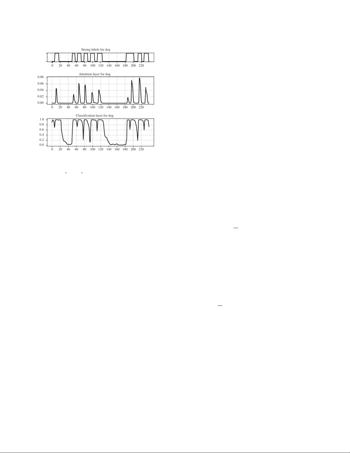
Detection and Classification of Acoustic Scenes and Events 2018 19-20 November 2018, Surre y , UK SOUND EVENT DETECTION USING WEAKL Y LABELLED SEMI-SUPER VISED D A T A WITH GCRNNS, V A T AND SELF-AD APTIVE LABEL REFINEMENT Robert Harb Graz Uni versity of T echnology , Austria robert.harb@student.tugraz.at F ranz P ernkopf Graz Uni versity of T echnology , Austria Signal Processing and Speech Communication Laboratory pernkopf@tugraz.at ABSTRA CT In this paper , we present a g ated con volutional recurrent neural net- work based approach to solve task 4, large-scale weakly labelled semi-supervised sound ev ent detection in domestic en vironments, of the DCASE 2018 challenge. Gated linear units and a tempo- ral attention layer are used to predict the onset and offset of sound ev ents in 10s long audio clips. Whereby for training only weakly- labelled data is used. V irtual adversarial training is used for regu- larization, utilizing both labelled and unlabelled data. Furthermore, we introduce self-adapti ve label refinement, a method which allo ws unsupervised adaption of our trained system to refine the accuracy of frame-level class predictions. The proposed system reaches an ov erall macro av eraged ev ent-based F-score of 34 . 6% , resulting in a relativ e improv ement of 20 . 5% ov er the baseline system. Index T erms — DCASE 2018, Con volutional neural net- works, Sound e vent detection, W eakly-supervised learning, Semi- supervised learning 1. INTR ODUCTION In this paper we summarize the methods we use to solve task 4 [1] of the DCASE 2018 challenge, the large-scale weakly labelled semi-supervised sound event detection in domestic envir onments . In contrast to audio tagging (A T), sound event detection (SED) not only requires to detect the presence of an event, but also a prediction about the temporal location in a given audio recording. Whereby in the data provided by the DCASE challenge, one input sequence pos- sibly contains multiple occurrences of different ev ent classes with potential temporal overlaps. Additionally , the training data is only weakly labelled. Therefore for training, the labels of each clip con- tain only information about the presence or absence of an e vent, b ut no strong labels which indicate the exact temporal onset and of fset. The proposed method uses a gated con volutional recurrent neu- ral network (GCRNN). This is similar to the best model of last years DCASE 2017 challenge task 4 [2] which also used a GCRNN based approach. Although, the objectiv e of the 2017 and 2018 DCASE challenge is SED, there are significant differences in the structure of the provided training data and ev aluation metric. More precisely , the following changes ha ve been made at the 2018 challenge: • The amount of weakly labelled training data is significantly smaller , 1,578 compared to 51,172. • In addition to the weakly labelled training set, there are unla- belled in-domain and unlabelled out-of-domain sets provided. • The domain of the ev ents is different: domestic envir onments compared to smart cars . Whereby the number of classes de- creased from 17 to 10. • For ev aluation, an event-based F-score with a 200ms collar on onsets and of fsets is used, instead of a segment-based error rate which is determined of one-second segments. W ith our work we show that a GCRNN based approach for SED similar to [2], is also suitable in a setting with the aforementioned differences. Whereby we introduce two major changes: First, to incorporate the provided unlabelled data we use virtual adversarial training (V A T) [3]. V A T has, amongst others, already been used successfully in semi-supervised text [4], image classifi- cation [3], acoustic ev ent detection [5] and phone classification [6] tasks. Furthermore, V A T showed competitive performance against other deep semi-supervised learning algorithms [7]. Secondly , as an extension to the attention mechanism we intro- duce an algorithm we call self-adaptiv e label refinement (SALR), which uses unlabelled input data and clip-level class predictions to refine the frame-lev el predictions of our model. 2. PR OPOSED METHOD 2.1. Gated con volutional r ecurrent neural network The winning team of last year’ s DCASE SED task [2] showed that using gated linear units (GLUs) [8] instead of commonly used acti- vation functions like rectified linear units (RELUs) or leak y ReLUs in the CRNN is a useful approach for SED. Gating mechanisms hav e been used successfully in a variety of neural network architectures. For example in RNNs using LSTM [9] cells, which have a separate input, output and forget gate. The rough idea behind gating mechanisms is to hav e a gate which can control how information flo ws in the network. In the setting of SED, the GLU units should adapt their be- haviour such that they act as an attention mechanism on the time- frequency (T -F) bin of each feature map. They can set their value close to one if information related to any of the considered audio ev ents passes through, and otherwise block the flow of unrelated information by setting their value close to zero. GLUs are defined as follows: Y = ( W ∗ X + b )  σ ( V ∗ X + c ) , (1) where W and V denote the con volutional filters with their respec- tiv e biases b and c , σ is the sigmoid function, X denotes the input to the layer , and  denotes elementwise multiplication. Detection and Classification of Acoustic Scenes and Events 2018 19-20 November 2018, Surre y , UK log mel spectogram - 64 bands - 240 frames conv , 3x3, 64 filters conv , 3x3, 64 filters max. pooling, 1x2 repeated 3 times batch normalization batch normalization linear activation sigmoid activation dropout, p=0.5 GRU fwd. path GRU GRU GRU ... GRU GRU GRU GRU ... bwd. path concat bidirectional RNN time distr . dense, sigmoid time distr . dense, softmax weighted average classification layer attention layer weak prediction 64 units 64 units cross entropy loss post-processing weak labels training inference strong pr ediction Figure 1: Network structure Figure 1 shows how the gated CNN blocks are incorporated into the network, whereby in our model we use three subsequent gated CNN blocks. The gated CNN blocks are followed by a bidirectional RNN containing 64 units in the forward and backward path, their output is concatenated and passed to the attention and classification layer which are described in Section 2.3. The final prediction y c for the weak label of class c is deter- mined by the weighted average of the element-wise multiplication of the attention and classification layer output of class c: y c = P T t z cla c ( t )  z att c ( t ) P T t z att c ( t ) , (2) where z cla c (t) and z att c (t) are the outputs of the classification layer and of the attention layer of class c. T denotes the frame-lev el res- olution of the input spectrogram, which is equal to the resolution of z cla c (t) and z att c (t), and t is the frame index. 2.2. V irtual adversarial training W e mak e use of V A T [3] for re gularization. W e calculate the virtual adversarial loss such that the robustness of the model’ s posterior distribution of predictions at clip-lev el p ( y | x ) is increased for small and bounded perturbations of the log-scaled mel-spectrograms x . The adversarial perturbation r v - adv is computed by maximizing a non-negati ve distance function between the unperturbed p ( y | x ; θ ) and perturbed p ( y | x + r ; θ ) posterior . Whereby θ denotes the cur- rent model parameter . The Kullback-Leibler di vergence KL is used as distance function between p ( y | x ; θ ) and p ( y | x + r ; θ ) , and || r || is limited to the sphere around x with some radius ≤  , i.e. r v - adv is determined as r v - adv = arg max r , k r k≤  KL [ p ( y | x ; θ ) || p ( y | x + r ; θ )] . (3) There is no evident closed-form solution for r v - adv , but [3] giv es a detailed deriv ation how to calculate an approximation of r v - adv . When using V A T the following additional cost is added to the objectiv e function: KL [ p ( y | x ; θ ) || p ( y | x + r v - adv ; θ )] . (4) Since calculating the virtual adversarial perturbation only requires input x and does not require label y , V A T is applicable to semi- supervised training. Therefore we use it to incorporate the unla- belled in-domain dataset into training. Howe ver , we decided not to include any of the provided unlabelled out-of-domain data since it has been shown previously that adding unlabelled data from differ - ent classes than the labelled data, can actually decrease the perfor- mance of semi-supervised learning algorithms like V A T [7]. 2.3. Attention mechanism T o predict the temporal locations of each audio event which is pre- sented in a giv en input sample, we use a similar approach as used in [2]. W e extend it by introducing self-adaptive label refinement based on weak and strong prediction alignment. This selects for each ev ent class an appropriate post-processing on the networks at- tention output. In the following the term weak prediction is used to refer to predictions at clip-lev el and strong prediction is used to refer to class predictions at frame-lev el. As depicted in Figure 1, the output of a bidirectional RNN is fed into both an attention and a classification layer . The classification layer uses a sigmoid activ ation function to predict the probability of each occurring class at each timestep. While the attention layer uses a softmax activ ation over all classes. Intuiti vely , using a softmax in the attention layer should aid the network to learn to pick the most dominant class at each frame. Although this might not be an ideal approach if temporal overlaps of multiple ev ents are occurring, since then a more dominant event might be able to suppress the activ ation of another one. Figure 2 shows the output of the classification and attention layer for one audio clip of the dev elopment set containing sev eral ev ents labelled as dog. It can be seen that there is a clear corre- lation between ground truth event labels and the activations of the attention and classification layer . Ho wev er it is not obvious how to extract the exact start and end points of each individual ev ent from the layer activ ations. Our experiments showed that just tak- ing the product of the attention and classification layer activ ations, Detection and Classification of Acoustic Scenes and Events 2018 19-20 November 2018, Surre y , UK 0 20 40 60 80 100 120 140 160 180 200 220 Strong labels for dog 0 20 40 60 80 100 120 140 160 180 200 220 0.00 0.02 0.04 0.06 0.08 Attention layer for dog 0 20 40 60 80 100 120 140 160 180 200 220 0.0 0.2 0.4 0.6 0.8 1.0 Classification laye r for dog Figure 2: Classification and attention layer activ ations for file: Y0a8RB5eOGJ4 30.000 40.000.wav and class dog. thresholded with a fixed value for all classes, e.g. 0 . 5 , giv es un- satisfactory results. Also it has been shown in similar weakly la- belled SED settings that the trained network adapts differently for different classes [10]. Especially there seems to be a difference be- tween classes which tend to have short ev ent durations in contrast to classes which span the majority of timesteps of a clip. Consider- ing this, it might be necessary to use a different post-processing for each class on the networks attention output to account for that. The fact that no strong event annotations are av ailable for training makes this a non-trivial problem, otherwise a simple approach would be to test se veral post-processing methods and select for each class the one which giv es the best performance. 2.4. Self-adaptive label r efinement (SALR) W e introduce self-adaptiv e label refinement, where we check the alignment between strong and weak predictions, and use this as an approximate prediction how well a giv en post-processing method performs at extracting the right onset and offset of events. Using this approach we can use unlabelled data to estimate how well a given post-processing parameterization performs for each class, and take the best performing parameterization for our final strong prediction. For post-proc essing we threshold the output value of the classi- fication layer , follo wed by a median filter . Therefore the parameters we v ary in each iteration are the threshold, and the width of the me- dian filter . Howe ver it should be noted that man y other methods for post-processing are possible, e.g. a second neural network which maps between the attention layer of the first network and strong predictions might be a potential approach. In particular, when training has finished, self-adaptiv e label re- finement repeats the following steps on each class with dif ferent post-processing parameterizations: 1. A full forward pass is performed to create weak and strong predictions for each clip. Whereby the follo wing steps are only carried out for clips where the weak prediction indicates occurrence of the current class. 2. Using the strong predictions, the spectrogram of each clip is split up into two groups of ne w samples. Each single ev ent occurrence of the examined class is extracted into new samples containing only the temporal frames of the spectrogram which possibly contains the event. Those new samples are labelled with 1 . Additionally , another sample is created which contains only the temporal frames of the original spectrogram where no occurrence of the giv en class was predicted. Those are all labelled to 0. 3. The generated new samples are then passed through the net- work. Using the resulting weak predictions and the labels assigned before, a crossentropy loss for each class is calcu- lated. This loss indicates ho w good the weak and strong pre- dictions align. Afterwards for each class, the post-processing with the smallest loss value is selected. This approach does not need any labels, neither strong nor weak. Therefore our method for post-processing selection is ap- plicable using data of both, the weakly-supervised and the unsu- pervised dataset. Also the method can be used to adapt the post- processing at inference time to new unseen data. 2.5. T raining The cross entropy loss between the predicted probabilities for each class and the weak ground truth labelling o ver all labelled clips in a batch is calculated as follows: E = − 1 N N X i M X c l ( i ) c log ( y ( i ) c ) , (5) where the number of classes is denoted by M, the number of weakly labelled 10 second audio clips by N, y ( i ) c denotes the predicted prob- ability for class c of sample i , and l ( i ) c is the given binary label in the weakly labelled train set. In each step a batch containing an equal distrib ution of samples from the labelled and unlabelled in-domain set is processed. The total loss consists of the cross entropy loss of the labelled samples, regularized with V A T depending on both the labelled and unlabelled samples weighted by a factor λ : L = − 1 N N X i M X c l ( i ) c log ( y ( i ) c ) + λ N 0 X i KL[ p ( y | x ( i ) ; θ ) || p ( y | x ( i ) + r ; θ )] , (6) where N 0 denotes the sum of labelled and unlabelled in-domain clips in a batch, x ( i ) is the log-scaled mel-spectrograms of a labelled or unlabelled in-domain clip with index i . The loss w as optimized using Adam [11] with a learning rate of 0 . 001 and a batch size of 30. The network was implemented using tensorflow [12]. 3. EXPERIMENTS AND RESUL TS 3.1. Dataset The method is e valuated using a subset of the Google Audioset [13], which was provided with task 4 of the DCASE 2018 challenge[14]. Detection and Classification of Acoustic Scenes and Events 2018 19-20 November 2018, Surre y , UK no V A T V A T challenge baseline no refinement SALR train SALR dev . no refinement SALR train SALR dev . Class F1 ER F1 ER F1 ER F1 ER F1 ER F1 ER F1 ER Alarm bell 3.2% - 27.0% 1.45 22.4% 1.18 18.8% 1.23 27.9% 1.38 21.0% 1.14 18.2% 1.12 Blender 15.4% - 18.5% 2.65 10.7% 1.25 26.9% 1.23 29.9% 1.52 23.2% 1.33 38.1% 0.97 Cat 0.0% - 9.5% 3.27 5.0% 1.40 33.5% 1.35 4.9% 2.87 19.2% 1.54 25.2% 1.30 Dishes 0.0% - 5.6% 1.65 0.0% 1.16 0.0% 1.16 29.3% 1.93 32.5% 1.16 32.5% 1.16 Dog 0.0% - 20.5% 2.16 18.5% 1.40 18.6% 1.39 7.4% 2.00 2.3% 1.36 15.8% 1.36 Elec. Shaver 32.4% - 18.4% 2.86 50.0% 0.86 50.0% 0.86 14.1% 2.61 40.0% 0.96 40.0% 0.96 Frying 31.0% - 20.4% 4.54 43.5% 1.62 42.9% 1.67 18.0% 3.79 40.0% 1.50 40.7% 1.46 Running water 11.4% - 17.5% 1.86 37.7% 1.00 38.0% 0.99 22.6% 1.89 31.1% 1.22 32.4% 1.21 Speech 0.0% - 36.5% 1.38 44.6% 0.95 36.2% 1.15 37.5% 1.25 41.3% 0.97 40.2% 0.98 V ac. cleaner 46.5% - 20.0% 3.11 48.8% 1.17 46.5% 1.28 21.8% 2.58 40.5% 1.31 63.0% 0.75 14.06% 1.54 19.4% 2.49 28.12% 1.19 31.2% 1.23 21.3% 2.18 29.1% 1.25 34.6% 1.12 T able 1: Class-wise results on the dev elopment set , total scores are macro averaged. The majority of the provided audioclips are 10 seconds long, a few audioclips are slightly shorter, for further processing we zero- pad those to a length of 10 seconds. Each audioclip contains one or multiple sound events of 10 different classes, whereby different ev ents may overlap. The dataset consists of a training, testing and ev aluation subset. The training subset consists of 1,578 weakly labelled clips, an unlabelled in-domain set of 14,412 clips and an unlabelled out-of- domain set of 39,999 clips extracted from classes that are not con- sidered in task 4. The test set contains 288 clips, whereby the distribution in terms of clips per class is similar to the weakly labelled training set. For the test set strong labels from human annotators are given, therefore timestamps for the onset and offset of each e vent in the clip are included. For training only weak labels are used. The weak labels indicate if a gi ven event occurs some where in a 10s clip, ho wev er no information about the onset and offset of the events, nor how often the event occurs is given. This setting can also be considered as a multiple instance learning (MIL) problem [10]. Log-scaled mel-spectrograms of each clip are passed as input to the network, for calculation the librosa library [15] is used. Before the spectrograms are calculated, each clip is con verted to a mono signal with a sampling rate of 16,000 Hz. For calculation of the log- scaled mel-spectrograms a hamming window of length 1024 with an ov erlap of 360 is used, this gi ves 240 frames with 64 mel frequency channels for each clip. 3.2. Baseline system The organizers of the DCASE challenge provided a baseline system for task 4 [1]. The system consists of two models based on the same structure: three con volution layers with 64 filters of size 3 × 3 , each one followed by a max pooling layer of size 4 × 1 and a dropout layer with p = 30% . After the con volutional layers, one bidirec- tional recurrent layer with 64 GR U units and 30% dropout on the input is placed. For output, the first model uses a dense layer with 10 sigmoid units and global a verage pooling across frames to mak e clip-lev el predictions, and the second model uses a time distributed dense layer with 10 sigmoid units to predict ev ents at frame-lev el. T raining of the system is performed in two steps: 1. The first model is trained with the weakly labelled training set, then the trained model is used to generate weak labels for the unlabelled in-domain set. 2. The second model is trained on the unlabelled in-domain set, using the weak labels generated beforehand. In this second training pass the weakly labelled set is used for validation. As input, each 10 second audio file is divided into 500 frames of 64 log mel-band magnitudes. 3.3. Evaluation For ev aluation the macro averaged ev ent-based F-score [16] is used. The event-based metrics are calculated using the open source tool- box sed ev al [17]. As given by the challenge, for calculation of ev ent-based metrics a 200ms collar on onsets and a 200ms / 20% of the ev ents length collar on offsets was set. For calculation of the total performance over all individual classes, macro av eraging is used. This has the effect that each class has equal influence on the final metrics, ev en if the distribution of classes in the tested set is unbalanced. 3.4. Results T able 1 shows the event based F1 scores and error rates of our sys- tem on the development set. W e compare the resulting scores of our system without post-processing refinement, and when we per- formed self-adaptiv e label refinement using data either of the train- ing or the development set. Additionally , we also show the influence of V A T . When no post-processing refinement was done, we calcu- lated the strong labels with a fixed threshold of 0 . 5 for all classes and apply no median filter . It can be seen that both SALR and V A T increase the performance of the system. Whereby when SALR is used, the best performance is achie ved when the adaption w as done on the dev elopment set. 3.5. Submitted systems Three systems have been submitted to the DCASE 2018 challenge, whereby self-adaptive label refinement was used to adapt the post- processing as follows: System one has been adapted to the evalu- ation set. System two did not use any adaption, but used the same post-processing with a fixed threshold of 0 . 5 and a median filter width of 1. System three has been adapted to the training set. 4. CONCLUSION In this paper, we proposed a method for sound event detection us- ing only weakly labelled and unsupervised data. Our approach is based on GCRNNs, whereby we introduce self-adaptiv e label re- finement. This method adapts the postprocessing using unlabelled data, and increases SED performance. The final F-score of our sys- tem is 34.6%, which is significantly higher than the score of the baseline system which is 14.06%. Detection and Classification of Acoustic Scenes and Events 2018 19-20 November 2018, Surre y , UK 5. REFERENCES [1] R. Serizel, N. T urpault, H. Eghbal-Zadeh, and A. Parag Shah, “Large-Scale W eakly Labeled Semi-Supervised Sound Event Detection in Domestic En vironments, ” in W orkshop on Detection and Classification of Acoustic Scenes and Events , W oking, United Kingdom, No v . 2018, sub- mitted to DCASE2018 W orkshop. [Online]. A vailable: https://hal.inria.fr/hal- 01850270 [2] Y . Xu, Q. K ong, W . W ang, and M. D. Plumbley , “Large- scale weakly supervised audio classification using gated con volutional neural network, ” in 2018 IEEE International Confer ence on Acoustics, Speec h and Signal Processing, ICASSP 2018, Calgary , AB, Canada, April 15-20, 2018 , 2018, pp. 121–125. [Online]. A vailable: https://doi.org/10. 1109/ICASSP .2018.8461975 [3] T . Miyato, S. Maeda, S. Ishii, and M. K oyama, “V irtual ad- versarial training: A regularization method for supervised and semi-supervised learning, ” IEEE T ransactions on P attern Analysis and Machine Intelligence , pp. 1–1, 2018. [4] T . Miayto, A. M. Dai, and I. Goodfellow , “V irtual adversarial training for semi-supervised text classification, ” 2016. [5] M. Z ¨ ohrer and F . Pernkopf, “V irtual adversarial training and data augmentation for acoustic ev ent detection with gated re- current neural networks, ” pp. 493–497, 08 2017. [6] M. Ratajczak, S. Tschiatschek, and F . Pernkopf, “V irtual ad- versarial training applied to neural higher-order factors for phone classification, ” in Interspeech , 2016. [7] A. Oliver , A. Odena, C. Raffel, E. D. Cubuk, and I. J. Goodfello w , “Realistic ev aluation of semi-supervised learning algorithms, ” 2018. [Online]. A v ailable: https: //openrevie w .net/forum?id=ByCZsFyPf [8] Y . N. Dauphin, A. Fan, M. Auli, and D. Grangier , “Language modeling with gated conv olutional networks, ” CoRR , v ol. abs/1612.08083, 2016. [Online]. A vailable: http://arxiv .or g/abs/1612.08083 [9] S. Hochreiter and J. Schmidhuber, “Long short-term memory , ” Neural Computation , vol. 9, no. 8, pp. 1735–1780, 1997. [Online]. A vailable: https://doi.org/10.1162/neco.1997. 9.8.1735 [10] B. McFee, J. Salamon, and J. P . Bello, “ Adapti ve pooling operators for weakly labeled sound ev ent detection, ” IEEE/A CM T rans. Audio, Speech and Lang. Pr oc. , vol. 26, no. 11, pp. 2180–2193, Nov . 2018. [Online]. A vailable: https://doi.org/10.1109/T ASLP .2018.2858559 [11] D. Kingma and J. Ba, “ Adam: A method for stochastic opti- mization, ” 12 2014. [12] M. Abadi, P . Barham, J. Chen, Z. Chen, A. Davis, J. Dean, M. Devin, S. Ghemawat, G. Irving, M. Isard, et al. , “T ensor- flow: a system for large-scale machine learning. ” [13] J. F . Gemmeke, D. P . Ellis, D. Freedman, A. Jansen, W . Lawrence, R. C. Moore, M. Plakal, and M. Ritter, “ Audio set: An ontology and human-labeled dataset for audio e vents, ” in Acoustics, Speech and Signal Pr ocessing (ICASSP), 2017 IEEE International Confer ence on . IEEE, 2017, pp. 776– 780. [14] http://dcase.community/workshop2018/. [15] B. McFee, C. Raffel, D. Liang, D. P . Ellis, M. McV icar, E. Battenberg, and O. Nieto, “librosa: Audio and music sig- nal analysis in python, ” in Pr oceedings of the 14th python in science confer ence , 2015, pp. 18–25. [16] A. Mesaros, T . Heittola, and T . V irtanen, “Metrics for polyphonic sound ev ent detection, ” Applied Sciences , vol. 6, no. 6, p. 162, 2016. [Online]. A vailable: http: //www .mdpi.com/2076- 3417/6/6/162 [17] A. Heittola, T .; Mesaros, “sed ev al - ev aluation toolbox for sound event detection. ” https://github .com/TUT - ARG/sed ev al, accessed: 2018-07-20.