Tensors, Learning, and Kolmogorov Extension for Finite-alphabet Random Vectors

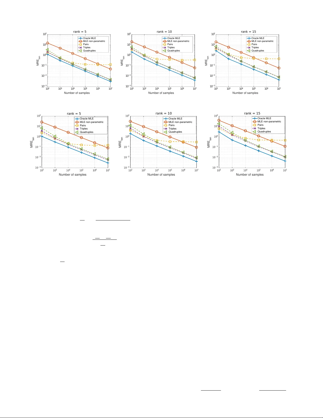
1 T ensors, Learning, and ‘K olmogoro v Extension’ for Finite-alphabet Random V ectors Nikos Karg as, Nicholas D. Sidiropoulos, F ellow , IEEE , and Xiao Fu, Member , IEEE Abstract —Estimating the joint probability mass function (PMF) of a set of random variables lies at the heart of statistical learning and signal pr ocessing. Without structural assumptions, such as modeling the variables as a Marko v chain, tree, or other graphical model, joint PMF estimation is often considered mission impossible – the number of unknowns grows exponentially with the number of variables. But who gives us the structural model? Is there a generic , ‘non-parametric’ way to control joint PMF complexity without r elying on a priori structural assumptions regarding the underlying probability model? Is it possible to discover the operational structure without biasing the analysis up front? What if we only observe random subsets of the variables, can we still reliably estimate the joint PMF of all? This paper shows, perhaps surprisingly , that if the joint PMF of any three variables can be estimated, then the joint PMF of all the variables can be prov ably recover ed under relatively mild conditions. The result is r eminiscent of Kolmogor ov’ s extension theorem – consistent specification of lower -dimensional distributions induces a unique probability measure for the entir e process. The differ ence is that f or pr ocesses of limited complexity (rank of the high-dimensional PMF) it is possible to obtain complete characterization fr om only thr ee- dimensional distributions. In fact not all thr ee-dimensional PMFs are needed; and under mor e stringent conditions even two- dimensional will do. Exploiting multilinear (tensor) algebra, this paper proves that such higher-dimensional PMF completion can be guaranteed – several pertinent identifiability results are derived. It also provides a practical and efficient algorithm to carry out the recovery task. Judiciously designed simulations and real-data experiments on movie recommendation and data classification are presented to showcase the effectiveness of the approach. Index T erms —Statistical learning, joint PMF estimation, tensor decomposition, rank, elementary probability , Kolmogor ov exten- sion, recommender systems, classification I . I N T RO D U C T I O N Estimating a joint Probability Mass Function (PMF) of a set of random v ariables is of great interest in numerous applications in the fields of machine learning, data mining and signal processing. In many cases, we are given partial observations and/or statistics of the data, i.e., incomplete data, marginalized lower -dimensional distributions, or lower - order moments of the data, and our goal is to estimate the missing data. If the full joint PMF of all variables of interest Original manuscript submitted to IEEE T rans. on Signal Pr ocessing Nov em- ber 30, 2017; revised April 24, 2018; accepted June 28, 2018. Supported in part by NSF IIS-1447788 and IIS-1704074. Conference version of part of this work appeared in Information Theory and Applications W orkshop 2017 [1]. N. Kargas is with the Dept. of ECE, Univ . of Minnesota, Minneapolis, MN 55455; N. D. Sidiropoulos is with the Dept. of ECE, Univ . of V ir ginia, Charlottesville, V A 22904; X. Fu is with the School of EE and CS, Oregon State Univ ersity , Corvallis, OR 97330. Author e-mails: karg a005@umn.edu, nikos@virginia.edu, xiao.fu@ore gonstate.edu were known, this would hav e been a straightforward task. A classical example is in recommender systems, where users rate only a small fraction of the total items (e.g., movies) and the objectiv e is to make item recommendations to users according to predicted ratings. If the joint PMF of the item ratings is known, such recommendation is readily implementable based on the conditional expectation or mode of the unobserved ratings given the observed ratings. A closely related problem is top- K recommendation, where the goal is to predict the K items that a user is most likely to b uy next. When the joint PMF of the items is known, it is easy to identify the K items with the highest individual or joint (‘bundle’) conditional probability given the observed user ratings. Another example is data classification. If the joint PMF of the features and the label is kno wn, then gi ven a test sample it is easy to infer the label according to the Maximum a P osteriori (MAP) principle. In fact, the joint PMF can be used to infer any of the features (or subsets of them), which is useful in imputing incomplete information in surveys or databases. Despite its importance in signal and data analytics, esti- mating the joint PMF is often considered mission impossible in general, if no structure or relationship between the v ari- ables (e.g., a tree structure or a Marko vian structure) can be assumed. This is true e ven when the problem size is merely moderate. The reason is that the number of unknown parameters is exponential in the number of v ariables. Consider a simple scenario of 10 v ariables taking 10 distinct values each. The number of parameters we need to estimate in this case is 10 10 . The ‘naiv e’ approach for joint PMF estimation is counting the occurences of the joint variable realizations. In practice, howe ver , when dealing with ev en moderately large sets of random variables, the probability of encountering any particular realization is v ery low . Therefore, only a small portion of the empirical distribution will be non-zero gi ven a reasonable amount of data samples – this makes the approach very inaccurate. In many applications, different workarounds have been proposed to circumvent this sample complexity problem. For example, in recommender systems, instead of trying to es- timate the joint PMF of the ratings (which w ould be the estimation-theoretic gold standard), the most popular approach is based on low-rank matrix completion [2], [3], [4]. The idea is that the users can be roughly clustered into se veral types, and users of the same type would rate dif ferent movies similarly . Consequently , the user-rating matrix is approximately lo w rank and this is used as prior information to infer the missing rat- ings. In classification, parsimonious function approximations are employed to model the relationship (or the conditional 2 users patients (Heart Desease) (Chol) (FBS) (Blood pressure) X X X X X X Dataset 1 (Inception) (The Matrix) (Star W ars) ( A vatar ) X X X X X X Dataset 2 Fig. 1: Applications of joint PMF estimation. T op: recom- mender systems: giv en partially observed ratings of a user on movies, we would like to infer the unobserved ratings. Bottom: classification problems: giv en medical features of people, we would like to infer if a person has heart disease. probability function) between the features and the label. Suc- cessful methods that fall into this category are support vector machines (linear function approximation), logistic regression (log-linear function approximation) and more recently kernels and neural networks (nonlinear function approximation) [5]. The above mentioned methods are nice and elegant, have triggered a tremendous amount of theoretical research and practical applications, and ha ve been successful in many ways. Howe ver , these workarounds hav e not yet answered our question of interest: Can we ever reliably estimate the joint PMF of v ariables given limited data? This question is very well-motiv ated in practice, since kno wledge of the joint PMF is indeed the gold standard: it enables optimal estimation under a v ariety of well-established criteria, such as mean-square error and minimum probability of error or Bayes risk. Kno wing the joint PMF can facilitate a lar ge v ariety of applications including recommender systems and classification in a unified and statistically optimal way , instead of resorting to often ad- hoc modeling tools. This paper sho ws, perhaps surprisingly , that if the joint PMF of any three variables can be estimated, then the joint PMF of all the v ariables can be provably recovered under relativ ely mild conditions. The result is reminiscent of Kol- mogorov’ s e xtension theorem – consistent specification of lower -dimensional distributions induces a unique probability measure for the entire process. The dif ference is that for processes of limited complexity (rank of the high-dimensional PMF) it is possible to obtain complete characterization from only three-dimensional distrib utions. In fact not all three- dimensional PMFs are needed; and under more stringent conditions e v en two-dimensional will do. The rank condi- tion on the high-dimensional joint PMF has an interesting interpretation: loosely speaking, it means that the random variables are ‘reasonably (in)dependent’. This mak es sense, because estimation problems in volving fully independent or fully dependent regressors and unknowns are contri ved – it is the middle ground that is interesting. It is also important to note that the marginal PMFs of triples can be reliably estimated at far smaller sample comple xity than the joint PMF of all variables. For e xample, for user-mo vie ratings, the marginal PMF of three giv en variables (movies) can be estimated by counting the co-occurrences of the giv en ratings (values of the v ariables) of the three given movies; but no user can rate all movies. Contributions Our specific contributions are as follows: • W e propose a nov el frame work for joint PMF estimation giv en limited and possibly very incomplete data samples. Our method is based on a nice and delicate connection between the Canonical Polyadic Decomposition (CPD) [6], [7] and the nai ve Bayes model. The CPD model, sometimes referred to as the Parallel Factor Analysis (P ARAF AC) model, is a popular analytical tool from multiway linear algebra. The CPD model has been used to model and analyze tensor data (data with more than two indices) in signal processing and machine learning, and it has found many successful applications, such as speech separation [8], blind CDMA detection [9], array processing [10], spectrum sensing and unmixing in cognitive radio [11], topic modeling [12], and community detection [13] – see the recent ov erview paper in [14]. Nev ertheless, CPD has never been considered as a statistical learning tool for recov ering a gener al joint PMF and our work is the first to establish the exciting connection 1 . • W e present detailed identifiability analysis of the proposed approach. W e first show that, any joint PMF can be represented by a naiv e Bayes model with a finite-alphabet latent variable – and the size of the latent alphabet (which happens to be the rank of the joint PMF tensor , as we will see) is bounded by a function of the alphabet sizes of the (possibly intermittently) observ ed v ariables. W e further show that, if the latent alphabet size is under a certain threshold, then the joint PMF of an arbitrary number of random variables can be identified from three-dimensional marginal distributions. W e prove this identifiability result by relating the joint PMF and marginal PMFs to the CPD model, which is known for its uniqueness ev en when the tensor rank is much larger than its outer dimensions. • In addition to the nov el formulation and identifiability results, we also propose an easily implementable joint PMF recov ery algorithm. Our identification criterion can be con- sidered as a coupled simplex-constrained tensor factoriza- tion problem, and we propose a very ef ficient alternating optimization-based algorithm to handle it. T o deal with the probability simplex constraints that arise for PMF estimation, the celebrated Alternating Direction Method of Multipliers (ADMM) algorithm is employed, resulting in lightweight iter- ations. Judiciously designed simulations and real experiments 1 There are works that considered using CPD to model a joint PMF for some specific problems [12]. Ho wev er , these works rely on specific physical interpretation of the associated model, which is sharply dif ferent to our setup – in which we employ the CPD model to explain a general joint PMF without assuming any physical model. 3 + + independent, rank=1 Fig. 2: It is impossible to recover the joint PMF from one- dimensional marginals without making strong assumptions. on movie recommendation and classification tasks are used to showcase the effecti veness of the approach. Preliminary version of part of this work appeared at IT A 2017 [1]. This journal version includes new and stronger identifiability theorems and interpretations, detailed analysis of the theorems, and insightful experiments on a number of real datasets. A. Notation Bold, lowercase and uppercase letters denote vectors and matrices respectively . Bold, underlined, uppercase letters de- note N -way ( N ≥ 3 ) tensors. Uppercase (lo wercase) let- ters denote scalar random variables (realizations thereof, re- spectiv ely). The outer product of N vectors is a N -way tensor with elements ( a 1 ◦ a 2 · · · ◦ a N )( i 1 , i 2 , . . . , i N ) = a 1 ( i 1 ) a 2 ( i 2 ) · · · a N ( i N ) . The Kronecker product of matrices A and B is denoted as A ⊗ B . The Khatri-Rao (column- wise Kronecker) product of matrices A and B is denoted as A  B . The Hadamard (element-wise) product of matrices A and B is denoted as A ~ B . W e define vec ( X ) the vector obtained by vertically stacking the elements of a tensor X into a vector . Additionally , diag ( x ) ∈ R I × I denotes the diagonal matrix with the elements of vector x ∈ R I on its diagonal. The set of integers S = { 1 , . . . , N } is denoted as [ N ] and |S | denotes the cardinality of the set S . I I . P RO B L E M S TA T E M E N T Consider a set of N random v ariables, i.e., { X n } N n =1 . Assume that each X n can take I n discrete values and only the joint PMFs of variable triples, i.e., Pr ( X j = i j , X k = i k , X ` = i ` ) ’ s, are av ailable. Can we identify the joint PMF of { X n } N n =1 , i.e., Pr ( X 1 = i 1 , . . . , X N = i N ) , from the three- dimensional marginals? This question lies at the heart of sta- tistical learning. T o see this, consider a classification problem and let X 1 . . . , X N − 1 represent the set of observed features, and X N the sought label. If Pr ( X 1 = i 1 , . . . , X N = i N ) is known, then given a specific realization of the features, one can easily compute the posterior probability Pr ( i N | i 1 . . . , i N − 1 ) = Pr ( i 1 , . . . , i N ) P I N i N =1 Pr ( i 1 , . . . , i N − 1 , i N ) , and predict the label according the MAP principle (here Pr ( i 1 , . . . , i N ) is shorthand for Pr ( X 1 = i 1 , . . . , X N = i N ) and lik ewise Pr ( i N | i 1 . . . , i N − 1 ) for Pr ( X N = i N | X 1 = i 1 . . . , X N − 1 = i N − 1 ) . In recommender systems, gi ven a Fig. 3: Bayesian network of three variables. set of observed item ratings X 1 . . . , X N − 1 one can compute the conditional expectation of an unobserved rating gi ven the observed ones E ( X N | i 1 , . . . , i N − 1 ) = I N X i N =1 i N Pr ( i N | i 1 , . . . , i N − 1 ) . At this point the reader may wonder why we consider recov ery from three-dimensional joint PMFs and not from one- or two-dimensional PMFs. It is well-known that re- cov ery from one-dimensional marginal PMFs is possible when all random v ariables are kno wn to be independent. In this case, the joint PMF is equal to the product of the individual one-dimensional marginals. Interestingly , recovery from one-dimensional mar ginals is also possible when the random variables are kno wn to be fully dependent i.e., one is completely determined by the other . In this case, the joint PMF can be recovered if each one-dimensional marginal is a unique permutation of the other . Howe v er , complete (in)dependence is unrealistic in sta- tistical estimation and learning practice. In general it is not possible to recov er a joint PMF from one-dimensional marginals. An illustration for two v ariables is shown in Fig- ure 2: Pr ( i 1 , i 2 ) can be represented as a matrix, and Pr ( i 1 ) , Pr ( i 2 ) are ‘projections’ of the matrix along the row and column directions using the projector 1 T and 1 , respecti vely: Pr ( i 1 ) = P I 2 i 2 =1 Pr ( i 1 , i 2 ) and Pr ( i 2 ) = P I 1 i 1 =1 Pr ( i 1 , i 2 ) . In this case, if we denote P the matrix such that P ( i 1 , i 2 ) = Pr ( X 1 = i 1 , X 2 = i 2 ) , then rank( P ) = r > 1 if X 1 and X 2 are not independent. From basic linear algebra, one can see that knowing 1 T P and P1 is not enough for recovering P in general – since this is equiv alent to solving a very underdetermined system of linear equations with ( I 1 + I 2 ) × r variables but only I 1 + I 2 equations. What if we kno w two-dimensional marginals? When the giv en random variables obey a probabilistic graphical model, and a genie re veals that model to us, then estimating a high- dimensional joint PMF from two-dimensional marginals may be possible. An example is shown in Figure 3. If we know a priori that random variables X 1 and X 2 are conditionally independent given X 3 , one can v erify that knowledge of Pr ( X 1 = i 1 , X 3 = i 3 ) and Pr ( X 2 = i 2 , X 3 = i 3 ) is sufficient to recov er Pr ( X 1 = i 1 , X 2 = i 2 , X 3 = i 3 ) . Ho wev er , this kind of approach hinges on knowing the probabilistic graph structure. Unfortunately , genies are hard to come by in real life, and learning the graph structure from data is itself a very challenging problem in statistical learning [15]. 4 Fig. 4: Illustration of the rank decomposition of a three-way tensor . In our problem setup, we do not assume any a priori knowledge of the graph structure, and in this sense we hav e a ‘blind’ joint PMF recovery problem. Interestingly , under certain conditions, this is no hindrance. I I I . P R E L I M I NA R I E S Our framework is hea vily based on lo w-rank tensor fac- torization and its nice identifiability properties. T o facilitate our later discussion, we briefly introduce pertinent aspects of tensors in this section. A. Rank Decomposition An N -way tensor X ∈ R I 1 × I 2 ×···× I N is a data array whose elements are index ed by N indices. A two-way tensor is a matrix, whose elements hav e two indices; i.e., X ( i, j ) denotes the ( i, j ) -th element of the matrix X . If a matrix X has rank F , it admits a rank decomposition X = P F f =1 A 1 (: , f ) ◦ A 2 (: , f ) = A 1 A T 2 where we have A n = [ A n (: , 1) , . . . , A n (: , F )] and ◦ denotes the outer product of two vectors, i.e., [ x ◦ y ]( i, j ) = x ( i ) y ( j ) . Similarly , if an N -way tensor X has rank F , it admits the following rank decomposition: X = F X f =1 A 1 (: , f ) ◦ A 2 (: , f ) ◦ · · · ◦ A N (: , f ) , (1) where A n ∈ R I n × F and F is the smallest number for which such a decomposition exists. For con v enience, we use the notation X = [ [ A 1 , . . . , A N ] ] to denote the decomposition. The above rank decomposition is also called the Canonical Polyadic Decomposition (CPD) or P arallel Factor Analysis (P ARAF A C) model of a tensor . It is critical to note that ev ery tensor admits a CPD, and that the rank F is not necessarily smaller than I 1 , . . . , I N – the latter is in sharp contrast to the matrix case [14]. In the matrix case, it is easy to see that X ( i 1 , i 2 ) = P F f =1 A 1 ( i 1 , f ) A 2 ( i 2 , f ) . Sim- ilarly , for an N -way tensor we hav e X ( i 1 , i 2 , . . . , i N ) = P F f =1 Q N n =1 A n ( i n , f ) . Sometimes one wishes to restrict the columns of A n ’ s to hav e unit norm (e.g., as in SVD). Therefore, the tensors can be represented as X = F X f =1 λ ( f ) A 1 (: , f ) ◦ A 2 (: , f ) ◦ · · · ◦ A N (: , f ) , (2) or , equiv alently X ( i 1 , i 2 , . . . , i N ) = F X f =1 λ ( f ) N Y n =1 A n ( i n , f ) , (3) where k A n (: , f ) k p = 1 for a certain p ≥ 1 , ∀ n, f , and λ = [ λ (1) , . . . , λ ( F )] T with k λ k 0 = F is employed to ‘absorb’ the norms of columns. An illustration of a three- way tensor and its CPD is sho wn in Figure 4. Under such cases, we denote the N -way tensor as X = [ [ λ , A 1 , . . . , A N ] ] – again, in this expression, we have automatically assumed that k A n (: , f ) k p = 1 , ∀ n, f and a certain p ≥ 1 . W e will refer to the decomposition of X into nonnegati ve factors λ ∈ R F + , A n ∈ R I n × F + as nonnegati ve decomposition. The following definitions will prov e useful in the rest of the paper . W e define the mode- n matrix unfolding of X as the matrix X ( n ) of size Q N k =1 k 6 = n I k × I n . W e hav e that X ( i 1 , i 2 , . . . , i N ) = X ( n ) ( j, i n ) , where j = 1 + N X k =1 k 6 = n ( i k − 1) J k with J k = k − 1 Y m =1 m 6 = n I m . In terms of the CPD factors, the mode- n matrix unfolding can be expressed as X ( n ) =    N  j =1 j 6 = n A j    diag ( λ ) A T n , (4) where N  j =1 j 6 = n A j = A N  · · ·  A n +1  A n − 1  · · ·  A 1 . W e can also express a tensor in a vectorized form X ( i 1 , i 2 , . . . , i N ) = x ( j ) , where j = 1 + N X k =1 ( i k − 1) J k with J k = k − 1 Y m =1 I m . In terms of the CPD factors, the vectorized form of a tensor can be expressed as vec ( X ) =  N  j =1 A j  λ . (5) B. Uniqueness of Rank Decomposition A distinctive feature of tensors is that they hav e essentially unique CPD under mild conditions – ev en when F is much larger than I 1 , . . . , I N . T o continue our discussion, let us first formally define what we mean by essential uniqueness of rank decomposition of tensors. Definition 1. (Essential uniqueness) F or a tensor X of (non- ne gative) rank F , we say that a nonnegative decomposition X = [ [ λ , A 1 , . . . , A N ] ] , λ ∈ R F + , A n ∈ R I n × F + is essentially unique if the factors ar e unique up to a common permutation. This means that if ther e exists another nonne gative decompo- sition X = [ [ b λ , b A 1 , . . . , b A N ] ] , then, ther e exists a permutation matrix Π such that b A n = A n Π , ∀ n ∈ [ N ] and b λ = Π T λ . In other words, if a tensor has an essentially unique non- negati ve CPD, then the only ambiguity is column permutation of the column-normalized factors { A n } N n =1 , which simply amounts to a permutation of the rank-one ‘chicken feet’ outer products (rank-one tensors) in Fig. 4, that is clearly 5 unav oidable 2 . Regarding the essential uniqueness of tensors, let us consider the three-way case first. The following is arguably the most well-known uniqueness condition that was rev ealed by Kruskal in 1977. Lemma 1. [16] Let X = [ [ λ , A 1 , A 2 , A 3 ] ] , wher e A 1 ∈ R I 1 × F , A 2 ∈ R I 2 × F , A 3 ∈ R I 3 × F . If k A 1 + k A 2 + k A 3 ≥ 2 F + 2 then rank ( X ) = F and the decomposition of X is essentially unique. Here, k A denotes the Kruskal rank of the matrix A which is equal to the largest integer such that e very sub- set of k A columns are linearly independent. Lemma 1 im- plies the following generic result: The decomposition X = [ [ λ , A 1 , A 2 , A 3 ] ] is essentially unique, almost surely , if min ( I 1 , F ) + min ( I 2 , F ) + min ( I 3 , F ) ≥ 2 F + 2 . (6) This is because k A n = min( I n , F ) with probability one if the elements of A n are generated following a certain absolutely continuous distrib ution. More relaxed and powerful uniqueness conditions hav e been proven in recent years. Lemma 2. [17], [18] Let X = [ [ λ , A 1 , A 2 , A 3 ] ] , where A 1 ∈ R I 1 × F , A 2 ∈ R I 2 × F , A 3 ∈ R I 3 × F , I 1 ≤ I 2 ≤ I 3 , I 1 ≥ 3 and F ≤ I 3 . Then, rank ( X ) = F and the decomposition of X is essentially unique, almost sur ely , if and only if F ≤ ( I 1 − 1)( I 2 − 1) . Lemma 3. [17] Let X = [ [ λ , A 1 , A 2 , A 3 ] ] , wher e A 1 ∈ R I 1 × F , A 2 ∈ R I 2 × F , A 3 ∈ R I 3 × F , I 1 ≤ I 2 ≤ I 3 . Let α, β be the lar gest inte gers such that 2 α ≤ I 1 and 2 β ≤ I 2 . If F ≤ 2 α + β − 2 then the decomposition of X is essentially unique almost sur ely . The condition also implies that if F ≤ ( I 1 +1)( I 2 +1) 16 , then X has a unique decomposition almost sur ely . There are many more dif ferent uniqueness conditions for CPD. The take-home point here is that the CPD model is essentially generically unique e ven if F is much larger than I 1 , I 2 , I 3 – so long it is less than maximal possible rank. For example, in Lemma 3, F can be as large as O ( I 1 I 2 ) (but not equal to I 1 I 2 ), and the CPD model is still unique. Remark 1. W e should mention that the abov e identifiability results are deriv ed for tensors under a noiseless setup 3 . In addition, although the results are stated for real factor matrices, they are very general and also cover nonnegativ e A n ’ s due to the fact that the nonnegati v e orthant has positiv e measure. It follows that if a tensor is generated using random nonnegati ve factor matrices then under the noiseless setup, a plain CPD can recover the true nonnegati ve factors. On the other hand, in practice, instead of considering exact tensor decomposition, often low-rank tensor appr oximation is of interest, because of limited sample size and other factors. The best low-rank tensor 2 Generally , there is also column scaling / counter-scaling ambiguity [14]: a red column can be multiplied by γ and the corresponding yellow col- umn divided by γ without any change in the outer product. There is no scaling ambiguity for nonne gative column-normalized representation X = [ [ λ , A 1 , . . . , A N ] ] , where there is obviously no sign ambiguity and all scaling is ‘absorbed’ in λ . 3 In this context, noise will typically come from insufficient sample aver- aging in empirical frequency estimation. approximation might not e ven exist in this case; fortunately , adding structural constraints on the latent factors can mitigate this, see [19]. In this work, our interest lies in rev ealing the fundamental limits of joint PMF estimation. Therefore, our analysis will be le veraging exact decomposition results, e.g., Lemmas 2-3. Howe ver , since the formulated problem natu- rally in v olves nonnegati ve latent factors, our computational framew ork utilizes this structural prior knowledge to enhance performance in practice. I V . N A I V E B AY E S M O D E L : A R A N K - D E C O M P O S I T I O N P E R S P E C T I V E W e will show that any joint PMF admits a naive Bayes model repr esentation , i.e., it can be generated from a latent variable model with just one hidden variable. The naiv e Bayes model postulates that there is a hidden discrete random variable H taking F possible values, such that giv en H = h the discrete random variables { X n } N n =1 are conditionally independent. It follows that the joint PMF of { X n } N n =1 can be decomposed as Pr ( i 1 , i 2 , . . . , i N ) = F X f =1 Pr ( f ) N Y n =1 Pr ( i n | f ) , (7) where Pr ( f ) := Pr ( H = f ) is the prior distribution of the latent v ariable H and Pr ( i n | f ) := Pr ( X n = i n | H = f ) are the conditional distributions (Fig. 5). The naiv e Bayes model in (7) is also referred to as the latent class model [20] and is the simplest form of a Bayesian network [15]. It has been employed in div erse applications such as classification [21], density estimation [22] and crowdsourcing [23], just to name a few . An interesting observation is that the naiv e Bayes model can be interpreted as a special nonnegati ve polyadic decom- position. This was alluded to in [24], [25] but not exploited for identifying the joint PMF from lo wer-dimensional marginals, as we do. Consider the element-wise representation in (3) and compare it with (7): each column of the factor matrices can represent a conditional PMF and the vector λ contains the prior probabilities of the latent variable H , i.e., A n ( i n , f ) = Pr ( i n | f ) , λ ( f ) = Pr ( f ) . (8) This is a special nonnegati ve polyadic decomposition model because it restricts 1 T λ = 1 . There is a subtle point howe ver: the maximal rank F in a CPD ( canonical polyadic decomposi- tion) model is bounded, but the number of latent states (latent alphabet size) for the naiv e Bayes model may exceed this bound. Ev en if the number of latent states is under the maximal rank bound, a naiv e Bayes model may be reducible , in the sense that there exists a naive Bayes model with fewer latent states that generates the same joint PMF . The net result is that every joint PMF admits a nai ve Bayes model interpr etation with bounded F , and every naiv e Bayes model is or can be reduced to a special CPD model. W e ha ve the following result. 6 Fig. 5: Naiv e Bayes model. Proposition 1. The maximum F needed to repr esent an arbitrary PMF as a naive Bayes model is bounded by the following inequality F ≤ min k    N Y n =1 n 6 = k I n    . (9) Pr oof: Let X ∈ R I 1 × I 2 × I 3 + denote a joint PMF of three random variables i.e., X ( i 1 , i 2 , i 3 ) = Pr ( X 1 = i 1 , X 2 = i 2 , X 3 = i 3 ) . W e define the following matrices A 1 := [ X (: , : , 1) , · · · , X (: , : , I 3 )] , A 2 := [ I I 2 × I 2 , · · · , I I 2 × I 2 ] = 1 T I 3 ⊗ I I 2 × I 2 , A 3 := I I 3 × I 3 ⊗ 1 T I 2 , where A 1 ∈ R I 1 × I 2 I 3 + , A 2 ∈ R I 2 × I 2 I 3 + , A 3 ∈ R I 3 × I 2 I 3 + and hav e used MA TLAB notation X (: , : , i 3 ) to denote the frontal slabs of the tensor X . Additionally , I I n × I n denotes the identity matrix of size I n × I n and 1 I n is a vector of all 1 ’ s of size I n . Then e very frontal slab of the tensor X can be synthesized as X (: , : , i 3 ) = A 1 diag ( A 3 ( i 3 , :)) A T 2 . Upon normalizing the columns of matrix A 1 such that they sum to one and absorbing the scaling in λ , i.e., A 1 = b A 1 diag( λ ) we can decompose the tensor as X = [ [ λ , b A 1 , A 2 , A 3 ] ] . The number of columns of each factor is I 2 I 3 . Due to role symmetry , by permuting the modes of the tensor it follows that we need at most min ( I 1 I 2 , I 2 I 3 , I 1 I 3 ) columns for each factor for exact decomposition. The result is easily generalized to a four -way tensor X ∈ R I 1 × I 2 × I 3 × I 4 + by noticing that each slab X (: , : , : , i 4 ) is a three-way tensor and thus can be decomposed as [ [ λ i 4 , b A 1 ,i 4 , A 2 ,i 4 , A 3 ,i 4 ] ] as before. W e define λ = [ λ T 1 , · · · , λ T I 4 ] T , b A 1 = [ b A 1 , 1 , · · · , b A 1 ,I 4 ] , A 2 = [ A 2 , 1 , · · · , A 2 ,I 4 ] , A 3 = [ A 3 , 1 , · · · , A 3 ,I 4 ] , A 4 = I I 4 ⊗ 1 T I 2 I 3 . The four-w ay tensor can therefore be decomposed as [ [ λ , b A 1 , A 2 , A 3 , A 4 ] ] . Due to symmetry , the number of columns of each factor is at most min ( I 1 I 2 I 3 , I 2 I 3 I 4 , I 1 I 3 I 4 , I 1 I 2 I 4 ) . By the same argument it follows that for a N -way tensor the bound on the nonnegativ e rank is min k ( Q N n =1 n 6 = k I n ) . The proof of Proposition 1 employs the same type of ar gument used to prove the upper bound on tensor rank. The main difference is in the normalization – latent Fig. 6: Rank and independence. nonnegati vity follows from data nonnegati vity “for free” since the latent factors used for constructing the CPD are either fibers drawn from the joint PMF itself, or from identity matrices or Kronecker products thereof. While the proof is fairly straightforward for someone versed in tensor analysis, the implication of this proposition to probability theory is significant: it asserts that every joint PMF can be represented by a naiv e Bayes model with a bounded number of latent states |H | . In fact, the connection between a naive Bayes model and CPD was utilized to approach some machine learning problems such as community detection and Gaussian Mixture Model (GMM) estimation in [13]. Howe ver , in those cases, the hidden v ariable has a specific physical meaning (e.g., H = f represents the f th community in community detection) and thus connection was established using a specific data generati v e model. Here, we emphasize that even when there is no physically meaningful H or presumed generative model, one can always r epr esent an arbitrary joint PMF , possibly corr esponding to a very complicated pr obabilistic graphical model, as a “simple” naive Bayes model with a bounded number of latent states F . This result is v ery significant, also because it spells out that the latent structure of a probabilistic graphical model cannot be identified by simply assuming few hidden nodes; one has to limit the number of hidden node states as well. W e should remark that although any joint PMF admits a naiv e Bayes representation, this does not mean that such repre- sentation is unique. Clearly , F needs to be strictly smaller than the upper bound in (9) to guarantee uniqueness (cf. Lemmas 1- 3). Fortunately , many joint PMFs that we encounter in practice are relatively lo w-rank tensors, since random variables in the real world are only moderately dependent. This leads to an in- teresting connection between linear dependence/independence and statistical dependence/independence. T o e xplain, let us consider the simplest case where N = 2 . In this case, we hav e Pr ( i 1 , i 2 ) = F X f =1 Pr ( f ) Pr ( i 1 | f ) Pr ( i 2 | f ) . (10) The two-way model corresponds to Nonnegati ve Matrix Fac- torization (NMF) and is related to Probabilistic Latent Se- mantic Indexing (PLSI) [26], [27]. For the two-way model, independence of the v ariables implies that the probability matrix is rank- 1 . On the other hand, when the v ariables 7 T ABLE I: Rel. error for dif ferent joint PMFs of 3 variables. Rank ( F ) 5 10 15 INCOME 2 . 1 × 10 − 2 5 . 5 × 10 − 3 5 . 1 × 10 − 3 MUSHR OOM 4 . 3 × 10 − 2 2 . 4 × 10 − 2 1 . 9 × 10 − 2 MO VIELENS 1 . 8 × 10 − 2 7 . 5 × 10 − 3 4 . 1 × 10 − 3 are fully dependent i.e., the v alue of one variable exactly determines the value of the other , the probability matrix is full- rank. Howe ver , low-rank does not necessarily mean that the variables are close to being independent as shown in Figure 6. There, a lo w rank probability matrix (rank = 2 ) can also model highly dependent random variables. In practice, we expect that random variables will be neither independent nor fully dependent and we are interested in cases where the rank of the joint PMF is lo wer (and ideally much lower) than the upper bound giv en in Proposition 1. As a sanity check, we conducted preliminary e xperiments on some real-life data. As anticipated, we verified that many joint PMFs are indeed low-rank tensors in practice. T able I sho ws interesting results: The joint PMF of three mo vies ov er 5 rating values was first estimated, using data from the MovieLens project. The joint PMF is then factored using a nonnegati ve CPD model with different rank v alues. One can see that with rank as low as 5 , the modeling error in terms of the relati ve error k X − b X k F / k X k F is quite small, meaning that the low- rank modeling is fairly accurate. The same applies to two more datasets drawn from the UCI repository . V . J O I N T P M F R E C OV E RY A. Gener al Pr ocedur es The key observation that enables our approach is that the marginal distribution of any subset of random variables is also a nonnegati ve CPD model. This is a direct consequence of the law of total probability . Marginalizing with respect to the k -th random variable we hav e that I k X i k =1 Pr ( i 1 , . . . , i N ) = F X f =1 I k X i k =1 Pr ( f ) N Y n =1 Pr ( i n | f ) = F X f =1 Pr ( f ) N Y n =1 n 6 = k Pr ( i n | f ) I k X i k =1 Pr ( i k | f ) = F X f =1 Pr ( f ) N Y n =1 n 6 = k Pr ( i n | f ) , (11) since P I n i n =1 Pr ( i n | f ) = 1 . Consider the model in (7) and assume that the mar ginal distributions Pr ( X j = i j , X k = i k , X l = i l ) , denoted Pr ( i j , i k , i l ) for brevity , ∀ j, k , l ∈ [ N ] , l > k > j are av ailable and perfectly known. Then, there e xists an exact decomposition of the form Pr ( i j , i k , i l ) = F X f =1 Pr ( f ) Pr ( i j | f ) Pr ( i k | f ) Pr ( i l | f ) . (12) The marginal distributions of triples of random variables satisfy X j kl = [ [ λ , A j , A k , A l ] ] , where { A n } N n =1 and λ are defined as in (8) and they satisfy A l ≥ 0 , A k ≥ 0 , A j ≥ 0 , 1 T A l = 1 T , 1 T A k = 1 T , 1 T A j = 1 T , λ > 0 , 1 T λ = 1 . Based on the connection between the naive Bayes model of lower -dimensional marginals and the joint PMF , we propose the following steps to recov er the complete joint PMF from three-dimensional marginals. Procedur e: Joint PMF Recovery From T riples [S1] Estimate X j k` from data; [S2] Jointly factor X j kl = [ [ λ , A j , A k , A l ] ] to estimate λ , A j , A k , A l ∀ j, k , l using a CPD model with rank F ; [S3] Synthesize the joint PMF X via Pr ( i 1 , i 2 , . . . , i N ) = P F f =1 Pr ( f ) Q N n =1 Pr ( i n | f ) , w/ Pr ( i n | f ) = A n ( i n , f ) , Pr ( f ) = λ ( f ) . One can see from step [S2], that if the individual factor- ization of at least one X j kl is unique, then the joint PMF is readily identifiable via [S3]. This is already very interesting. Howe v er , as we will sho w in Sec. VI, we may identify the joint PMF ev en when the marginal tensors do not have unique CPD. The reason is that many marginal tensors share factors and we can exploit this to come up with much stronger identifiability results. B. Algorithm: Coupled Matrix/T ensor F actorization Before we discuss theoretical results such as identifiability of the joint PMF using three or higher-dimensional marginals, we first propose an implementation of [S2] in the proposed procedure. For brevity , we assume we hav e estimates of three- dimensional marginal distrib utions, i.e., we are gi v en empirical estimates b Pr ( X j = i j , X k = i k , X l = i l ) , ∀ j, k , l ∈ [ N ] , l > k > j , which we put in a tensor X j kl i.e., X j kl ( i j , i k , i l ) = b Pr ( X j = i j , X k = i k , X l = i l ) . The method can be easily generalized to any type of low- dimensional marginal distributions. Under the assumption of a lo w-rank CPD model, ev ery empirical marginal distribution of three random variables can be approximated as follows b Pr ( i j , i k , i l ) ≈ F X f =1 Pr ( f ) Pr ( i j | f ) Pr ( i k | f ) Pr ( i l | f ) . (13) Therefore, in order to compute an estimate of the full joint PMF , we propose solving the following optimization problem min { A n } N n =1 , λ X j X k>j X l>k 1 2   X j kl − [ [ λ , A j , A k , A l ] ]   2 F subject to λ ≥ 0 , 1 T λ = 1 , A n ≥ 0 , n = 1 , . . . , N , 1 T A n = 1 T , n = 1 , . . . , N . (14) The optimization problem in (14) is an instance of coupled tensor factorization. Coupled tensor/matrix factorization is usually used as a way of combining various datasets that share dimensions and corresponding factor matrices [28], [29]. Notice that in the case where we ha ve estimates of two-dimensional marginals, the optimization problem in (14) corresponds to coupled matrix factorization. The optimization 8 Algorithm 1 Coupled T ensor Factorization Approach Input : A discrete valued dataset D ∈ R M × N Output : Estimates of { A n } N n =1 and λ 1: Estimate X j,k,l ∀ j, k , l ∈ [ N ] , l > k > j from data. 2: Initialize { A n } N n =1 and λ such that the probability sim- plex constraints are satisfied. 3: r epeat 4: for all n ∈ [ N ] do 5: Solve optimization problem (16) 6: end for 7: Solve optimization problem (17) 8: until con v ergence criterion satisfied problem per se is very challenging and deserves developing sophisticated algorithms for handling it: first, when the number of random variables ( N ) gets large, there is a large number of optimization v ariables (i.e., { A n } N n =1 ) to be determined in (14) – and each A n is an I n × F matrix where I n (the alphabet size of the n -th random variable) can be large. In addition, the probability simplex constraints impose some extra computational burden. Nev ertheless, we found that, by carefully re-arranging terms, the formulated problem can be recast in conv enient form and handled in a way that is reminiscent of the classical alternating least squares algorithm with constraints. The idea is that we cyclically update variables { A n } N n =1 and λ while fixing the remaining variables at their last updated values. Assume that we fix estimates λ , A n , ∀ n ∈ [ N ] \ { j } . Then, the optimization problem with respect to A j becomes min A j X k 6 = j X l 6 = j l>k 1 2   X j kl − [ [ λ , A j , A k , A l ] ]   2 F subject to A j ≥ 0 , 1 T A j = 1 T . (15) Note that we hav e dropped the terms that do not depend on A j . By using the mode- 1 matrix unfolding of each tensor X j kl , the problem can be equi valently written as min A j X k 6 = j X l 6 = j l>k 1 2    X (1) j kl − ( A l  A k ) diag ( λ ) A T j    2 F subject to A j ≥ 0 , 1 T A j = 1 T , (16) which is a least-squares problem with respect to matrix A j under probability simplex constraints on its columns. The optimization problem has the same form for each factor A n due to role symmetry . In order to update λ we solve the following optimization problem min λ X j X k>j X l>k 1 2   vec ( X j kl ) − ( A l  A k  A j ) λ   2 2 subject to λ ≥ 0 , 1 T λ = 1 . (17) Both Problems (16) and (17) are linearly constrained quadratic programs, and can be solved to optimality by many standard solvers. Here, we propose to employ the Alternating Dir ection Method of Multipliers (ADMM) to solve these two sub-problems because of its flexibility and ef fectiv eness in handling large-scale tensor decomposition [30], [31]. Details of the ADMM algorithm for solving Problems (16)-(17) can be found in the Appendix B. The whole procedure is listed in Algorithm 1. As mentioned, the algorithm is easily modified to cover the cases where higher-dimensional marginals or pairwise marginals are giv en, and thus these cases are omitted. V I . J O I N T P M F I D E N T I FI A B I L I T Y A N A L Y S I S In this section, we study the conditions under which we can identify Pr ( i 1 , . . . , i N ) from marginalized lo wer-dimensional distributions. For brevity , we focus on three-dimensional as lower -dimensional distributions, and ev en though many more results are possible, we concentrate here on the case I n = I ∀ n ∈ [ N ] for ease of exposition and manuscript length con- siderations. Similar type of analysis applies when I 1 , . . . , I N are different, howe ver the analysis should be customized to properly address particular cases. Our aim here is to conv ey the spirit of what is possible in terms of identifiability results, as we cannot provide an exhausti ve treatment (there are combinatorially many cases, clearly). Obviously , if X j kl is individually identifiable for each combination of j, k , l , then, Pr ( i j | f ) , Pr ( i k | f ) , Pr ( i l | f ) , and Pr ( f ) are identifiable. This means that gi ven three-dimensional marginal distributions, Pr ( i 1 , . . . , i N ) is generically identifi- able if F ≤ 3 I − 2 2 assuming that I n = I ∀ n ∈ [ N ] . This can be readily sho wn by in voking Lemma 1, equation (6), and the link between the naiv e Bayes model and tensor factorization discussed in Sec. IV. Note that F ≤ 3 I − 2 2 is already not a bad condition, since in many cases we have approximately low-rank tensors in practice. Howe ver , since we have many factor -coupled X j kl ’ s, this identifiability condition can be significantly improved. W e hav e the following theorems. Theorem 1. Assume that Pr ( i n | f ) , ∀ n ∈ [ N ] are drawn fr om an absolutely continuous distrib ution, that I 1 = . . . = I N = I , and that the joint PMF Pr ( i 1 , . . . , i N ) can be r epr esented using a naive Bayes model of rank F . If N ≤ I then, Pr ( i 1 , . . . , i N ) is almost surely (a.s) identifiable fr om the Pr ( i j , i k , i l ) ’ s if F ≤ I ( N − 2) If N > I then, Pr ( i 1 , . . . , i N ) is a.s. identifiable fr om the Pr ( i j , i k , i l ) ’ s if F ≤  b √ N I − 1 I c I − 1  2 Pr oof: The proof is relegated to Appendix A. Theorem 2. Assume that Pr ( i n | f ) , ∀ n ∈ [ N ] are drawn fr om an absolutely continuous distribution, that I 1 = . . . = I N = I , and that the joint PMF Pr ( i 1 , . . . , i N ) can be repr esented using a naive Bayes model of rank F . Let α be the lar gest inte ger such that 2 α ≤ b N 3 c I . Then, Pr ( i 1 , . . . , i N ) is a.s. identifiable fr om the Pr ( i j , i k , i l ) ’ s if F ≤ 4 α − 1 which is implied by F ≤ ( b N 3 c I + 1) 2 16 . 9 T ABLE II: Rank bounds for generic identifiability ( I = 3) . Number of V ariables ( N ) 6 10 20 40 80 T riples 4 7 27 105 410 Quadruples 10 36 179 729 2916 T ABLE III: Rank bounds for generic identifiability ( N = 6) . Alphabet size ( I ) 6 10 20 40 80 T riples 24 40 105 410 1620 Quadruples 45 131 544 2220 8966 Pr oof: The proof is relegated to Appendix A. The rank bounds in Theorems 1-2 are nontrivial, albeit far from the maximal attainable rank for the cases considered. Recalling that higher-order tensors are identifiable for higher ranks, a natural question is whether kno wledge of four- or higher-dimensional marginals can further enhance identifiabil- ity of the complete joint PMF . The next theorem shows that the answer is affirmati ve. Theorem 3. Assume that Pr ( i n | f ) , ∀ n ∈ [ N ] are drawn fr om an absolutely continuous distrib ution, that I 1 = . . . = I N = I , and that the joint PMF Pr ( i 1 , . . . , i N ) can be r epr esented using a naive Bayes model of rank F . Further assume that S = [ N ] can be partitioned into 4 disjoint subsets de- noted by S 1 , . . . , S 4 such that the four-dimensional marginals Pr ( i j , i k , i l , i m ) , ∀ j ∈ S 1 , ∀ k ∈ S 2 , ∀ l ∈ S 3 , ∀ m ∈ S 4 ar e available. Then, the joint PMF Pr ( i 1 , . . . , i N ) is a.s. identifiable if F ≤ I 2 |S 3 ||S 4 | , 2 F ( F − 1) ≤ I 2 |S 1 ||S 2 | ( I |S 1 | − 1)( I |S 2 | − 1) . Pr oof: The proof is relegated to Appendix A. The conditions of Theorem 3 are satisfied for much higher rank than those of Theorems 1-2 as sho wn in T ables II-III. The results related to the four-dimensional marginals are obtained following Theorem 3 via checking all possible partitions. The cav eat is that one may need many more samples to reliably estimate the four -dimensional marginals. Nevertheless, the theorems that we present in this section offer insights regarding the choice of lo wer-dimensional mar ginals to work with – such choice depends on the size of the alphabet of each variable ( I ) and the number of variables ( N ) as well as the amount of av ailable data samples. Remark 2. The abov e results rely on Lemmas 2, 3 and concern the identifiability of a generic choice of parame- ters; i.e., the parameters are assumed to be drawn randomly from a jointly continuous distribution. At this point one may wonder whether this is a realistic assumption in practice. For example, in some latent model identification problems a hidden variable has specific physical meaning and an observed variable may not depend on the state of the hidden v ariable for one or more of its values. Consider a Hidden Markov Model (HMM) where we denote the observ ed v ariable at time t as X t and the hidden state is S t . The conditional T ABLE IV: Mean relative factor and tensor error when lower - dimensional marginals are perfectly known. Rank MRE fact MRE ten Pairs 0 . 277 0 . 148 F = 5 Triples 1 . 18 × 10 − 7 4 . 58 × 10 − 8 Quadruples 3 . 39 × 10 − 8 1 . 19 × 10 − 8 Pairs 0 . 440 0 . 187 F = 10 Triples 3 . 58 × 10 − 7 8 . 70 × 10 − 8 Quadruples 1 . 26 × 10 − 7 2 . 58 × 10 − 8 Pairs 0 . 466 0 . 184 F = 15 Triples 6 . 77 × 10 − 7 1 . 52 × 10 − 7 Quadruples 1 . 78 × 10 − 7 3 . 57 × 10 − 8 distribution e A t ( i, s ) := Pr ( X t = i | S t = s ) may be the same for tw o dif ferent v alues s 1 and s 2 of the hidden state S t . In such a case, the Kruskal rank of matrix e A t would be equal to 1 , thereby rendering the deterministic identifiability condition (Lemma 1) useless. Do note, howe ver , that in our setting the latent variable H does not necessarily have a physical interpretation; the CPD is just a conv enient ‘uni versal’ parametrization of the joint PMF . Therefore the conditional distribution of an observed variable may be the same for two values of the hidden state, but it may still depend on the value of the ‘virtual’ global latent variable H , and hence recovery of the the joint PMF using lower-dimensional marginals could still be possible. V I I . N U M E R I C A L R E S U L T S In this section, we employ judiciously designed synthetic data simulations to sho wcase the effecti v eness of the proposed joint PMF recovery methods. W e also apply the approach to real-data problems such as classification and recommender systems to demonstrate its usefulness in real machine learning tasks. A. Synthetic-Data Simulations W e first e valuate the proposed approach using synthetic data. W e consider a case where N = 5 random v ariables are present, and each variable can take I n = 10 discrete v alues. W e assume that the joint PMF of the 5 random variables can be represented by a naiv e Bayes model whose latent variable H can take F v alues, where F is set to be { 5 , 10 , 15 } . W e generate matrices A n ∈ R I n × F + , that model the conditional probabilities i.e., A n ( i n , f ) = Pr ( i n | f ) . A vector λ ∈ R F + is also generated for the latent random variable H such that λ ( f ) = Pr ( f ) . The elements of each A n and the vector λ are drawn independently from a uniform distribution between zero and one, and each column is normalized to sum to 1 . The ground-truth joint PMF is then constructed following the naiv e Bayes model, i.e., Pr ( i 1 , . . . , i 5 ) = X ( i 1 , . . . , i 5 ) = P F f =1 λ ( f ) Q 5 n =1 A n ( i n , f ) . W e assume that the observable data are two-, three- and four-dimensional marginals of the joint PMF . Under such settings, we can verify if the proposed procedure and algorithm can effecti vely reco ver the joint PMF , if there is no modeling error and the joint PMF does have low rank. W e run 20 Monte Carlo simulations and compute the 10 1 0 2 1 0 3 1 0 4 1 0 5 1 0 6 1 0 7 Number of samples 1 0 − 3 1 0 − 2 1 0 − 1 1 0 0 1 0 1 1 0 2 MRE ten rank = 5 Or acle ML E MLE non-parametric Pairs Triples Quadruples 1 0 2 1 0 3 1 0 4 1 0 5 1 0 6 1 0 7 Number of samples 1 0 − 3 1 0 − 2 1 0 − 1 1 0 0 1 0 1 1 0 2 MRE ten rank = 10 Or acle ML E MLE non-parametric Pairs Triples Quadruples 1 0 2 1 0 3 1 0 4 1 0 5 1 0 6 1 0 7 Number of samples 1 0 − 3 1 0 − 2 1 0 − 1 1 0 0 1 0 1 1 0 2 MRE ten rank = 15 Or acle ML E MLE non-parametric Pairs Triples Quadruples Fig. 7: Mean relative error of the estimated joint PMF under different number of av ailable samples. Number of samples MRE ten Or acle ML E MLE non-parametric Pairs Triples Quadruples rank = 5 Number of samples MRE ten Or acle ML E MLE non-parametric Pairs Triples Quadruples rank = 10 Number of samples MRE ten Or acle ML E MLE non-parametric Pairs Triples Quadruples rank = 15 Fig. 8: Mean relative error of the estimated joint PMF under different number of av ailable samples. mean relative error of the factors as well as the mean relativ e error of the recovered tensor which are defined as follows MRE fact = E 1 N N X n =1 k A n − b A n Π k F k A n k F ! , MRE ten = E k X − b X k F k X k F ! , where Π is a permutation matrix to fix the permutation ambiguity , and b X , b A n are the estimated joint PMF and the corresponding conditional PMFs. T able IV shows the mean relativ e errors for estimating the conditional PMFs and joint PMF using the dif ferent types of input under dif ferent choices of rank. Consistent with our analysis, one can see that using mar ginal distributions of triples or quadruples of random variables (i.e., three- and four- dimensional marginals) we are able to recover the joint PMF of 5 random variables. Here recov ery with high accuracy has been demonstrated; exact recov ery is also possible in certain cases, see [14]. Howe v er , using pairs (i.e., two-dimensional marginals) is not as promising. Recall that our identifiability result is built upon the identifiability of third- and higher-order CPD models. These nice identifiability results in general do not hold for matrices – which explains the sharp performance difference between using the pairs and higher-dimensional marginals. Pairs can work, howe ver , when the conditional probability matrices are suf ficiently sparse, and under more stringent constraints on the rank F . W e defer detailed discus- sion to a follow up paper , due to lack of space in this one. The abo ve simulation serves as sanity check – if the av ailable data and the model perfectly match with each other and we hav e noiseless marginal distrib utions, the proposed approach can indeed recover the joint PMF . In practice, we usually do not have exact estimates of the lower -dimensional marginal distributions. Next, we provide a set of more realistic simulations where we estimate the marginal PMFs using sample av erages from the observed data. 1) Fully-observed data: W e follow the same way of gener- ating the ground-truth joint PMF as in the previous simulation. Then, drawing from the joint PMF , we generate a synthetic dataset of M fiv e-dimensional data points. The data is gener- ated as follows: for each data point, we first draw a sample h m according to λ ; i.e., a realization of the hidden variable H . Then the data point (vector) s m = [ s m (1) , . . . , s m ( N )] T is generated by drawing its elements independently from { A n } (: , h m ) N n =1 , i.e., s m ( n ) is drawn from { A n } (: , h m ) . This is equiv alent to synthesizing the five-w ay joint PMF tensor and drawing an outcome from it (cf. the nai ve Bayes interpretation). W e use the generated 5 -dimensional data points to estimate lower -dimensional marginals and run our ADMM algorithm to recover the full joint PMF . W e repeat for a total of 10 Monte Carlo simulations. Figure 7 sho ws the tensor mean relativ e error of the estimated joint PMF under different dataset sizes M . W e also include the performance of two additional methods for estimating the joint PMF . Giv en the full data together with ‘oracle’ observations of the hidden variable H , we perform Maximum Likelihood Estimation (MLE) of the naiv e Bayes parameters, denoted as oracle MLE, which is done simply by frequency counting Pr ( f ) M L = coun t( f ) M , Pr ( i n | f ) M L = coun t( i n , f ) coun t( f ) , 11 T ABLE V: Misclassification error on dif ferent UCI datasets. Binary Multiclass Method INCOME CREDIT HEAR T MUSHR OOM VO TES CAR NURSER Y CP (Pairs) 0 . 177 ± 0 . 004 0 . 134 ± 0 . 019 0 . 151 ± 0 . 023 0 . 010 ± 0 . 007 0 . 046 ± 0 . 024 0 . 128 ± 0 . 021 0 . 101 ± 0 . 009 CP (T riples) 0 . 175 ± 0 . 003 0 . 129 ± 0 . 018 0 . 147 ± 0 . 031 0 . 006 ± 0 . 002 0 . 043 ± 0 . 024 0 . 089 ± 0 . 016 0 . 069 ± 0 . 011 CP (Quadruples) 0.171 ± 0 . 003 0.123 ± 0 . 018 0.138 ± 0 . 029 0 . 002 ± 0 . 001 0 . 042 ± 0 . 020 0 . 074 ± 0 . 015 0 . 061 ± 0 . 007 SVM (Linear) 0 . 179 ± 0 . 004 0 . 146 ± 0 . 027 0 . 170 ± 0 . 053 0 ± 0 0.038 ± 0 . 025 0 . 065 ± 0 . 006 0 . 063 ± 0 . 004 SVM (RBF) 0 . 174 ± 0 . 004 0 . 136 ± 0 . 018 0 . 187 ± 0 . 055 0 ± 0 0 . 079 ± 0 . 024 0.026 ± 0 . 008 0.006 ± 0 . 001 Naiv e Bayes 0 . 209 ± 0 . 005 0 . 140 ± 0 . 018 0 . 166 ± 0 . 026 0 . 044 ± 0 . 005 0 . 096 ± 0 . 022 0 . 151 ± 0 . 016 0 . 097 ± 0 . 007 T ABLE VI: Dataset information. Dataset N F INCOME 8 [1 , 20] CREDIT 9 [1 , 20] HEAR T 9 [1 , 10] MUSHR OOM 22 [1 , 20] V O TES 17 [1 , 10] CAR 7 [1 , 15] NURSER Y 9 [1 , 15] where count( i n , f ) is the number of times that X n = i n and H = f appear together in the dataset and count(f ) the number of times H takes the value f . W e also include the MLE of a non-parametric approach in which we use the empirical 5 - dimensional distribution as our estimate i.e., Pr ( i 1 , . . . , i N ) M L = coun t( i 1 , . . . , i N ) M . One can see that the estimation performance of our method is similar under different rank values and approaches that of oracle MLE using three- and four-dimensional marginals. In addition, as expected, the recovery accuracy steadily improves as the size of the a vailable dataset increases. On the other hand, when using two-dimensional marginals the performance improv es until it reaches a plateau at approximately M = 10 5 . The ability to recover the joint PMF using pairs of random variables is obviously limited by identifiability of matrix factorization. 2) Missing data: W e repeat the abov e e xperiment when some of the dataset entries are missing. W e randomly hide 20% of the data and compute estimates of two- three- and four-dimensional marginals using only the av ailable data. W e run the ADMM-based algorithm and repeat for 10 Monte Carlo simulations. The estimation performance of our method is again similar under different rank values and approaches that of oracle MLE. As expected, we observe a slight decrease in performance which is due to the less accurate estimation of the lower-dimensional marginals. In this case, the MLE non- parametric method takes into account only the fully observed samples. Note that when empirical estimates of the lower - dimensional distributions are used and the number of samples is limited, three-dimensional distributions may gi ve lower relativ e error compared to the four-dimensional ones. This shows that in some cases using lower -dimensional distrib utions can be more beneficial than higher-order ones in terms of parameter estimation accuracy . Actually , this is not very sur- prising since it can be shown that empirical lower -dimensional marginals are always more accurate than higher-dimensional ones when estimated given the same data [32]. B. Real-Data Experiments In real applications, the ground-truth joint PMF and the conditional PMFs are not kno wn. Nev ertheless, we can ev al- uate the method on a variety of standard machine learning tasks to observe its effecti veness. In this subsection, we test the proposed approach on two different tasks, namely , data classification and recommender systems. Note that both tasks can be easily accomplished if the joint PMF of pertinent variables (e.g., features and labels in classification) is kno wn and thus are suitable for ev aluating our method. Note that the rank of the joint PMF tensor , or , F = |H | , cannot be known as in the simulations. Fortunately , this is a single discrete v ariable that can be easily tuned, e.g., via observing v alidation errors as in machine learning. 1) Classification T ask: W e e valuate the performance of our approach on 7 different datasets from the UCI machine learn- ing repository [33]. Fi ve of the selected datasets correspond to binary classification and two to multi-class classification. For each dataset, we represent the training samples using its discrete features so that the PMF-based approach can be applied. W e split each dataset such that 70% of the data samples is used for training, 10% used for validation and 20% for testing. For each dataset, we let X N be the label and X 1 , . . . , X N − 1 be the selected features. W e estimate lower -dimensional marginal distributions of pairs, triples and quadruples of variables using the samples in the training set. Then, we use the marginals to estimate Pr ( i n | f ) , and Pr ( f ) . After applying the proposed approach for estimating the joint PMF , we predict for each data point of the test set the corresponding label using the MAP rule. The MAP estimator of the label l ( s m ) of the m -th observation s m = [ s m (1) , . . . , s m ( N − 1)] T in the test set can be written as b l map ( s m ) = arg max i N ∈{ 1 ,...,I N } Pr ( i N | s m (1) , . . . , s m ( N − 1)) , where I N is the number of classes. Equiv alently , using the Bayes rule the above can be found by b l map ( s m ) = arg max i N ∈{ 1 ,...,I N } F X f =1 Pr ( f ) Pr ( i N | f ) N − 1 Y n =1 Pr ( s m ( n ) | f ) . For each dataset, we run 10 Monte Carlo simulations with randomly partitioned training/validation/test sets and observe the av erage result. As mentioned, we do not know a priori 12 T ABLE VII: RMSE and MAE of different algorithms on MovieLens (Ratings are in the range [1-5]). MovieLens Dataset 1 MovieLens Dataset 2 MovieLens Dataset 3 Method RMSE MAE RMSE MAE RMSE MAE CP (Pairs) 0 . 802 ± 0 . 003 0 . 608 ± 0 . 003 0 . 795 ± 0 . 002 0 . 611 ± 0 . 002 0 . 897 ± 0 . 003 0 . 702 ± 0 . 002 CP (T riples) 0 . 783 ± 0 . 002 0 . 591 ± 0 . 002 0.785 ± 0.002 0.599 ± 0.002 0 . 887 ± 0 . 002 0 . 691 ± 0 . 002 CP (Quadruples) 0 . 778 ± 0 . 002 0 . 588 ± 0 . 002 0 . 786 ± 0 . 002 0 . 600 ± 0 . 002 0.884 ± 0.002 0.689 ± 0.002 Global A verage 0 . 945 ± 0 . 001 0 . 693 ± 0 . 001 0 . 906 ± 0 . 002 0 . 653 ± 0 . 002 0 . 996 ± 0 . 002 0 . 798 ± 0 . 001 User A verage 0 . 879 ± 0 . 002 0 . 679 ± 0 . 001 0 . 830 ± 0 . 003 0 . 625 ± 0 . 002 1 . 010 ± 0 . 002 0 . 768 ± 0 . 002 Movie A verage 0 . 886 ± 0 . 002 0 . 705 ± 0 . 001 0 . 889 ± 0 . 002 0 . 673 ± 0 . 002 0 . 942 ± 0 . 002 0 . 754 ± 0 . 001 BMF 0 . 797 ± 0 . 002 0 . 623 ± 0 . 002 0 . 792 ± 0 . 002 0 . 604 ± 0 . 002 0 . 904 ± 0 . 003 0 . 701 ± 0 . 003 what is an appropriate rank for our model. Therefore, for each dataset, we fit models of different rank values and choose the one which minimizes the misclassification error of the validation set as in standard machine learning practice. W e use 3 different classical classifiers from the MA TLAB Statistics and Machine Learning T oolbox as baselines; linear SVM, kernel SVM with radial basis function and a nai ve Bayes classifier . For SVM classifiers, we use both the original data encoding as well as the one-hot encoding which usually is more suitable for discrete data and report the best result among the two. Note that the baseline naiv e Bayes approach is very different from ours: the baseline method assumes that the features are independent given the label, while we assume that the label and the features are independent given an unknown latent variable. The former is a very strong assumption that is rarely satisfied by real data, but our assumption holds for an arbitrary set of random v ariables provided F is large enough, as we showed in Proposition 1. T able V shows the classification errors obtained on the datasets. One can see that our approach outperforms the naiv e Bayes classifier which assumes that the features are independent giv en the label. Sev eral observations are in or- der . First, using higher-dimensional marginals, the proposed approach giv es better classification results compared to using lower -dimensional ones. This is consistent with our analysis in Sec. VI – higher-dimensional marginals lead to stronger ov erall identifiability of the joint PMF . One can see that for all the datasets under test, using four-dimensional marginal distributions giv es the best classification accuracy compared to the three- and two-dimensional ones. Second, for the fiv e binary classification experiments, the proposed method works better than (on three datasets) or comparable to the baselines. This is quite surprising since our method does not directly optimize a classification criterion as SVM does. The result suggests that the proposed method indeed captures the essence of the joint distribution and the recovered joint PMF can be utilized to make inference in practice. Third, for the multiclass datasets, the proposed method yields accuracy that is less than the SVM methods. This also makes sense: when X N has a value set whose cardinality grows from 2 to 5, the joint PMFs of X N and X i , X j for i, j < N require more samples to estimate accurately . This also shows an interesting sample complexity-accuracy trade-of f of the proposed method. Nev ertheless, the method still works comparably well with the linear SVM, which supports the usefulness of the joint PMF estimation method. 2) Recommender Systems: W e also ev aluate the method for the task of recommender systems using the MovieLens dataset [34]. MovieLens is a dataset that contains ratings on 5 -star scale, with half-star increments, by a number of users. In order to test our algorithm we select three dif ferent subsets of the full dataset and round the ratings to the next integer . Initially , three different categories (action, animation and romance) are selected. From each category we extract a user -by-rating submatrix by keeping the 20 most rated movies and form the 3 datasets for our experiments. Note that the constructed three datasets hav e many missing v alues, since not all users w atched and rated all movies. The task of recommender systems is to recommend unwatched movies to users based on prediction of the user’ s rating gi ven the av ailable data. W e aim at estimating the joint PMF of the movie ratings. In this case, each random variable X n represents a movie, and it takes values from { 1 , . . . , 5 } , i.e., the ratings. Consequently , the joint PMF is a twenty-way tensor which has 5 20 elements. The 3 partially observed datasets are used in order to estimate lower -dimensional marginal distributions of pairs, triples and quadruples of the variables (movies). W e use the estimated PMF to compute the expected value of users’ ratings that we do not observe giv en the ones we observe. More specifically , let s m = [ s m (1) , . . . , s m ( N )] be the ratings of the m -th user and s m ( N ) = 0 i.e., the user has a missing rating. The conditional expectation of the movie’ s rating is giv en by b s N = I N X i N =1 i N Pr ( i N | s m (1) , . . . , s m ( N − 1)) . As a baseline algorithm, we use the Biased Matrix Factoriza- tion (BMF) method [2], which is a commonly used method in recommender systems. The BMF method is essentially low- rank matrix completion with modifications. Additionally , we present results obtained by global av erage of the ratings, the user average, and the item av erage as baselines for predicting the missing entries. For each dataset we randomly hide 20% ratings that we use as a test set, 10% ratings that we use as a validation set and the remaining dataset is used as a training set. W e run 10 Monte Carlo simulations using our approach and the BMF algorithm. W e select the parameters of both methods based on the RMSE of the validation set. T able VII shows the performance of the two algorithms in terms of the RMSE and Mean Absolute Error (MAE). One can see that, for the three datasets under test, the proposed method and the BMF method output clearly lower RMSEs and MAEs relativ e to the naiv e methods using averaging. In addition, the 13 proposed method slightly outperforms BMF on all of the three datasets. Note that BMF is considered a state-of-art method for movie recommendation, and it incorporates application- specific custom features, such as user bias and mo vie bias to achieve good performance. The proposed method, on the other hand, only uses basic probability to handle the same task – it is completely application-blind. This suggests that the joint PMF modeling and the proposed algorithm are both quite ef fectiv e. Last, we also observe accuracy improv ement when we increase the dimension of the marginal distributions used in the approach. Again, this performance may come from the identifiability gain as we analyzed in Theorem 3. V I I I . C O N C L U S I O N S In this work, we ha ve taken a fresh look at one of the most fundamental problems in statistical learning – joint PMF estimation. Due to the curse of dimensionality , naiv e count- based estimation is mission impossible in most cases. One popular approach has historically been to assume a plausible structural model, such as a Markov chain, tree, or other prob- abilistic graphical model, and do inference using this model. W e sho wed that a very different ‘non-parametric’ tensor-based approach is possible, and it features se veral ke y benefits. Foremost among them is guaranteed identifiability of the high-dimensional joint PMF from low-dimensional marginals, which can be reliably estimated using counting from much fewer examples, e ven if there are (many) samples missing from each e xample. This ability to infer a unique higher- dimensional joint PMF by specifying lower -dimensional ones is reminiscent of Kolmogoro v extension, which is intuitiv ely very pleasing. W e have also pro ven two more results that appear fun- damental and close to the heart of probability and learning theory: i) every joint PMF can be interpr eted as a nai ve Bayes model; and ii) probabilistic graphical models, which are very popular in statistical and computer science, are never identifiable if one simply limits the number of hidden nodes; one needs to bound the number of hidden states as well. Our non-parametric approach can re veal the true hidden structure, instead of assuming it; and this alleviates the risk of up-front bias in the analysis. On the practical side, our approach is appealing since lo wer- dimensional marginals can be more reliably estimated from a limited amount of partially observ able data. W e have also provided a practical and easily implementable algorithm that is based on factor-coupled tensor factorization to handle the recov ery problem. Simulations and judicious experiments with real data hav e sho wn that the performance of the proposed approach is consistent with our analysis, and approaches or exceeds that of state-of-art application-specific solutions that hav e come out after years of intensiv e research, which is satisfying. A P P E N D I X A I D E N T I FI A B I L I T Y R E S U LT S A. Pr oof of Theor em 1 Each three-dimensional marginal satisfies X j kl = [ [ λ , A j , A k , A l ] ] , where A l ≥ 0 , A k ≥ 0 , A j ≥ 0 , 1 T A l = 1 T , 1 T A k = 1 T , 1 T A j = 1 T , λ > 0 , 1 T λ = 1 . Consider a partition of the set S = [ N ] into three disjoint sets S 1 , S 2 , S 3 and define the following factors b A 1 = [ A T u 1 , · · · , A T u |S 1 | ] T b A 2 = [ A T v 1 , · · · , A T v |S 2 | ] T b A 3 = [ A T w 1 , · · · , A T w |S 3 | ] T (18) with u t ∈ S 1 , v t ∈ S 2 , w t ∈ S 3 . Then, we can construct a single virtual nonnegati ve CPD model b X (1) = ( b A 3  b A 2 ) diag ( λ ) b A T 1 , (19) where b A 1 ∈ R I |S 1 |× F + , b A 2 ∈ R I |S 2 |× F + , b A 3 ∈ R I |S 3 |× F + and b X ∈ R I |S 1 |× I |S 2 |× I |S 3 | + . W e hav e used a subset of the a vailable information to synthesize a virtual single nonne gati ve CPD model of size I 1 × I 2 × I 3 , with I k := I |S k | . Therefore, we can apply identifiability results of three-way tensors. W e observe that the sizes of the dif ferent modes of the virtual tensor depend on the way we partition the variables. W e distinguish between two cases and apply Lemma 2. 1) ( N ≤ I ) : W e partition the variables into three sets such that I 1 = I , I 2 = I and I 3 = ( N − 2) I . Clearly we have that I 3 > I 2 , I 1 and I 3 < ( I 1 − 1)( I 2 − 1) . According to Lemma 2 tensor b X admits unique decomposition for F ≤ min ( I 3 , ( I 1 − 1)( I 2 − 1)) = ( N − 2) I . 2) ( N > I ) : In this case we can partition the variables into three sets such that I 3 = ( I 1 − 1)( I 2 − 1) . W e can always hav e that I 1 = I 2 . The equality is satisfied when |S 1 | = |S 2 | = √ ( N I − 1) I . According to Lemma 2 tensor b X admits unique decomposition for F ≤ min( I 3 , ( I 1 − 1)( I 2 − 1)) ≤ ( b √ ( N I − 1) I c I − 1) 2 . B. Pr oof of Theor em 2 As abo ve, but this time choosing |S 1 | = |S 2 | = b N 3 c , | S 3 | = N − 2 | S 1 | and in voking Lemma 3. C. Pr oof of Theor em 3 Consider a partitioning the variables into four disjoint sets similar to the three-way case. W e obtain a single nonnegati ve CPD of the following form X (1) = ( b A 4  b A 3  b A 2 ) diag ( λ ) b A T 1 , which is a fourth-order tensor b X ∈ R I |S 1 |× I |S 2 |× I |S 3 |× I |S 4 | + . A fourth-order tensor can be viewed as a third-order tensor of size I |S 1 | × I |S 2 | × I 2 |S 4 ||S 3 | with a specially structured factor matrix. W e can write the mode- 1 unfolding of the tensor b X as b X (1) = ( ¯ A 3  b A 2 ) diag ( λ ) b A T 1 , (20) where ¯ A 3 = b A 4  b A 3 . Lemmas 2-3 cannot be applied in this case because of the Khatri-Rao structure of one factor . W e will use the following result Lemma 4. [35] Let X = [ [ A 1 , A 2 , A 3 ] ] , wher e A 1 ∈ R I 1 × F , A 2 ∈ R I 2 × F , A 3 ∈ R I 3 × F . If rank ( A 3 ) = F and 14 rank  M 2 ( A 1 )  M 2 ( A 2 )  =  F 2  , then rank ( X ) = F and the decomposition is essentially unique. M 2 ( A ) denotes the  I 2  ×  F 2  compound matrix containing all 2 × 2 minors of A . The generic version of Lemma 4 states that if F ≤ I 3 and 2 F ( F − 1) ≤ I 1 ( I 1 − 1) I 2 ( I 2 − 1) , then the decomposition of X is essentially unique, a.s. [36]. W e know that a Khatri-Rao product of two matrices is full rank almost surely [37, Corollary 1]. For the three-way tensor in (20) we hav e I 1 = I |S 1 | , I 2 = I |S 2 | and I 3 = I 2 |S 3 ||S 4 | . Applying the generic version of Lemma 4 we obtain the desired result. A P P E N D I X B A L G O R I T H M W e reformulate optimization problem (16) by introducing an auxiliary v ariable b A j . The problem can be equiv alently written as min A j , b A j f ( b A j ) + r ( A j ) subject to A j = b A T j (21) where f ( b A j ) = X k 6 = j X l 6 = j l>k 1 2    X (1) j kl − ( A l  A k ) diag ( λ ) b A j    2 F , r ( A ) is the indicator function for the probability simple x constraints C = { A | A ≥ 0 , 1 T A = 1 T } r ( A ) = ( 0 , A ∈ C ∞ , A / ∈ C . Optimization problem (21) can be readily solved by applying the ADMM algorithm. W e solve for A j by performing the following updates b A ( τ +1) j = ( G j + ρ I ) − 1  V j + ρ  A ( τ ) j + U ( τ ) j  T  , A ( τ +1) j = P C  A ( τ ) j − b A ( τ +1) T j + U ( τ ) j  , U ( τ +1) j = U ( τ ) j + A ( τ +1) j − b A ( τ +1) T j , where G j = ( λλ T ) ~ X k 6 = j X l 6 = j l>k Q T lk Q lk , V j = diag ( λ ) X k 6 = j X l 6 = j l>k Q T lk X (1) j kl , Q lk = A l  A k . P C is the projection operator onto the con ve x set C and τ de- notes the iteration index. V arious methods exist for projecting onto the probability simplex, e.g., see [38]. Note that in order to ef ficiently compute matrix G j we use a property of the Khatri-Rao product; Q T lk Q lk = ( A T l A l ) ~ ( A T k A k ) . Efficient algorithms also exist for the computation of matrix V j which is a sum of Matricized T ensor T imes Khatri-Rao Product (MTTKRP) terms [39], [40]. Similarly , we can deriv e updates for λ . At each ADMM iteration we perform the following updates b λ ( τ +1) = ( G + ρ I ) − 1  V + ρ  λ ( τ ) + u ( τ )  , λ ( τ +1) = P C  λ ( τ ) − b λ ( τ +1) + u ( τ )  , u ( τ +1) = u ( τ ) + λ ( τ +1) − b λ ( τ +1) . where G = X j X k>j X l>k Q T lkj Q lkj , V = X j X k>j X l>k Q T lkj vec ( X j kl ) , Q lkj = A l  A k  A j . R E F E R E N C E S [1] N. Kargas and N. D. Sidiropoulos, “Completing a joint PMF from projections: a low-rank coupled tensor factorization approach, ” in Proc. IEEE IT A , Feb . 2017. [2] Y . Koren, R. Bell, and C. V olinsky , “Matrix f actorization techniques for recommender systems, ” Computer , vol. 42, no. 8, pp. 30–37, Aug. 2009. [3] P . Jain, P . Netrapalli, and S. Sanghavi, “Low-rank matrix completion using alternating minimization, ” in Pr oc. 45th Annu. ACM Symp. Theory Comput. , 2013, pp. 665–674. [4] A. Mnih and R. R. Salakhutdinov , “Probabilistic matrix factorization, ” in Pr oc. Adv . Neural Inf. Pr ocess. Syst. , 2008, pp. 1257–1264. [5] C. M. Bishop, P attern reco gnition and machine learning . Springer , 2006. [6] J. D. Carroll and J. J. Chang, “ Analysis of individual differences in multidimensional scaling via an n-way generalization of Eckart-Y oung decomposition, ” Psychometrika , vol. 35, no. 3, pp. 283–319, Sep. 1970. [7] R. A. Harshman, “Foundations of the P ARAF A C procedure: Models and conditions for an ”explanatory” multimodal factor analysis, ” UCLA W orking P aper s Phonetics , vol. 16, pp. 1–84, 1970. [8] D. Nion, K. N. Mokios, N. D. Sidiropoulos, and A. Potamianos, “Batch and adaptiv e P ARAF A C-based blind separation of con voluti ve speech mixtures, ” IEEE T rans. Audio, Speech, Lang. Process. , vol. 18, no. 6, pp. 1193–1207, Aug. 2010. [9] N. D. Sidiropoulos, G. B. Giannakis, and R. Bro, “Blind P ARAF AC receiv ers for DS-CDMA systems, ” IEEE T rans. Signal Pr ocess. , vol. 48, no. 3, pp. 810–823, Mar . 2000. [10] N. D. Sidiropoulos, R. Bro, and G. B. Giannakis, “Parallel f actor analysis in sensor array processing, ” IEEE Tr ans. Signal Process. , vol. 48, no. 8, pp. 2377–2388, Aug. 2000. [11] X. Fu, N. D. Sidiropoulos, J. H. T ranter , and W .-K. Ma, “ A factor analysis framew ork for power spectra separation and multiple emitter localization, ” IEEE T rans. Signal Process. , vol. 63, no. 24, pp. 6581– 6594, Aug. 2015. [12] A. Anandkumar , R. Ge, D. Hsu, S. M. Kakade, and M. T elgarsk y , “T ensor decompositions for learning latent variable models, ” J. Mach. Learn. Res. , vol. 15, no. 1, pp. 2773–2832, Aug. 2014. [13] A. Anandkumar , R. Ge, D. Hsu, and S. M. Kakade, “ A tensor approach to learning mixed membership community models, ” J. Mach. Learn. Res. , vol. 15, no. 1, pp. 2239–2312, Jan. 2014. [14] N. D. Sidiropoulos, L. De Lathauwer, X. Fu, K. Huang, E. E. Papalex- akis, and C. Faloutsos, “T ensor decomposition for signal processing and machine learning, ” IEEE T rans. Signal Pr ocess. , vol. 65, no. 13, pp. 3551–3582, Jul. 2017. [15] D. Koller and N. Friedman, Probabilistic graphical models: principles and techniques . MIT Press, 2009. [16] J. B. Kruskal, “Three-way arrays: rank and uniqueness of trilinear decompositions, with application to arithmetic complexity a nd statistics, ” Linear Algebra Appl. , v ol. 18, no. 2, pp. 95–138, 1977. [17] L. Chiantini and G. Ottaviani, “On generic identifiability of 3-tensors of small rank, ” SIAM J. Matrix Anal. Appl. , vol. 33, no. 3, pp. 1018–1037, 2012. [18] I. Domanov and L. D. Lathauwer , “Generic uniqueness conditions for the canonical polyadic decomposition and INDSCAL, ” SIAM J . Matrix Anal. Appl. , vol. 36, no. 4, pp. 1567–1589, 2015. [19] Y . Qi, P . Comon, and L.-H. Lim, “Semialgebraic geometry of nonneg- ativ e tensor rank, ” SIAM J ournal on Matrix Analysis and Applications , vol. 37, no. 4, pp. 1556–1580, 2016. 15 [20] N. L. Zhang, “Hierarchical latent class models for cluster analysis, ” J. Mach. Learn. Res. , v ol. 5, no. 6, pp. 697–723, Jun. 2004. [21] A. Y . Ng and M. I. Jordan, “On discriminative vs. generativ e classifiers: A comparison of logistic regression and naive Bayes, ” in Proc. Adv . Neural Inf . Pr ocess. Syst. , 2002, pp. 841–848. [22] D. Lowd and P . Domingos, “Naiv e Bayes models for probability estimation, ” in Pr oc. Int. Conf. Mach. Learn. , 2005, pp. 529–536. [23] A. P . Dawid and A. M. Skene, “Maximum likelihood estimation of observer error-rates using the EM algorithm, ” Applied Statistics , vol. 28, no. 1, pp. 20–28, 1979. [24] A. Shashua and T . Hazan, “Non-negati ve tensor factorization with applications to statistics and computer vision, ” in Pr oc. Int. Conf. Mach. Learn. , 2005, pp. 792–799. [25] L.-H. Lim and P . Comon, “Nonnegati ve approximations of nonne gativ e tensors, ” J . Chemometr . , v ol. 23, no. 7-8, pp. 432–441, Jul. 2009. [26] T . Hofmann, “Probabilistic latent semantic indexing, ” in Proc. 22nd Annu. Int. ACM SIGIR Conf. Res. Develop. Inf. Retrieval , 1999, pp. 50–57. [27] E. Gaussier and C. Goutte, “Relation between PLSA and NMF and implications, ” in Pr oc. 28th Annu. Int. ACM SIGIR Conf. Res. Develop. Inf. Retrieval , 2005, pp. 601–602. [28] A. Beutel, P . P . T alukdar , A. Kumar , C. Faloutsos, E. E. Papalexakis, and E. P . Xing, “FlexiFact: Scalable flexible factorization of coupled tensors on hadoop, ” in Proc. SIAM Int. Conf. Data Mining , 2014, pp. 109–117. [29] E. Acar, T . G. Kolda, and D. M. Dunlavy , “ All-at-once optimization for coupled matrix and tensor factorizations, ” in Proc. KDD W orkshop Min. Learn. Graphs , 2011. [30] K. Huang, N. D. Sidiropoulos, and A. P . Liav as, “ A flexible and efficient algorithmic framework for constrained matrix and tensor factorization, ” IEEE Tr ans. Signal Pr ocess. , vol. 64, no. 19, pp. 5052–5065, 2016. [31] X. Fu, K. Huang, W .-K. Ma, N. D. Sidiropoulos, and R. Bro, “Joint tensor factorization and outlying slab suppression with applications, ” IEEE Tr ans. Signal Pr ocess. , vol. 63, no. 23, pp. 6315–6328, 2015. [32] K. Huang, X. Fu, and N. D. Sidiropoulos, “Learning Hidden Markov Models from Pairwise Co-occurrences with Applications to T opic Mod- eling, ” ArXiv pr eprint arXiv:1802.06894 , Feb . 2018. [33] M. Lichman, “UCI machine learning repository , ” 2013. [Online]. A vailable: http://archiv e.ics.uci.edu/ml [34] F . M. Harper and J. A. Konstan, “The MovieLens datasets: History and context, ” ACM Tr ans. Inter . Intel. Systems , vol. 5, no. 4, pp. 1–19, Dec. 2016. [35] T . Jiang and N. D. Sidiropoulos, “Kruskal’s permutation lemma and the identification of CANDECOMP/P ARAF A C and bilinear models with constant modulus constraints, ” IEEE T r ans. Signal Pr ocess. , vol. 52, no. 9, pp. 2625–2636, Sep. 2004. [36] A. Stegeman, J. M. T . Berge, and L. D. Lathauwer, “Sufficient condi- tions for uniqueness in CANDECOMP/P ARAF A C and INDSCAL with random component matrices, ” Psychometrika , vol. 71, no. 2, pp. 219– 229, 2006. [37] T . Jiang, N. D. Sidiropoulos, and J. M. F . ten Berge, “ Almost-sure identifiability of multidimensional harmonic retriev al, ” IEEE T rans. Signal Process. , vol. 49, no. 9, pp. 1849–1859, Sep. 2001. [38] W . W ang and M. A. Carreira-Perpin ´ an, “Projection onto the probability simplex: An efficient algorithm with a simple proof, and an application, ” ArXiv preprint arXiv:1309.1541 , 2013. [39] B. W . Bader and T . G. K olda, “Efficient matlab computations with sparse and factored tensors, ” SIAM J. Sci. Comp. , vol. 30, no. 1, pp. 205–231, 2008. [40] S. Smith, N. Ravindran, N. D. Sidiropoulos, and G. Karypis, “SPLA TT: Efficient and parallel sparse tensor-matrix multiplication, ” in IEEE Inter . P ar . Dist. Process. Symposium , May 2015, pp. 61–70.