Deep Long Short-Term Memory Adaptive Beamforming Networks For Multichannel Robust Speech Recognition

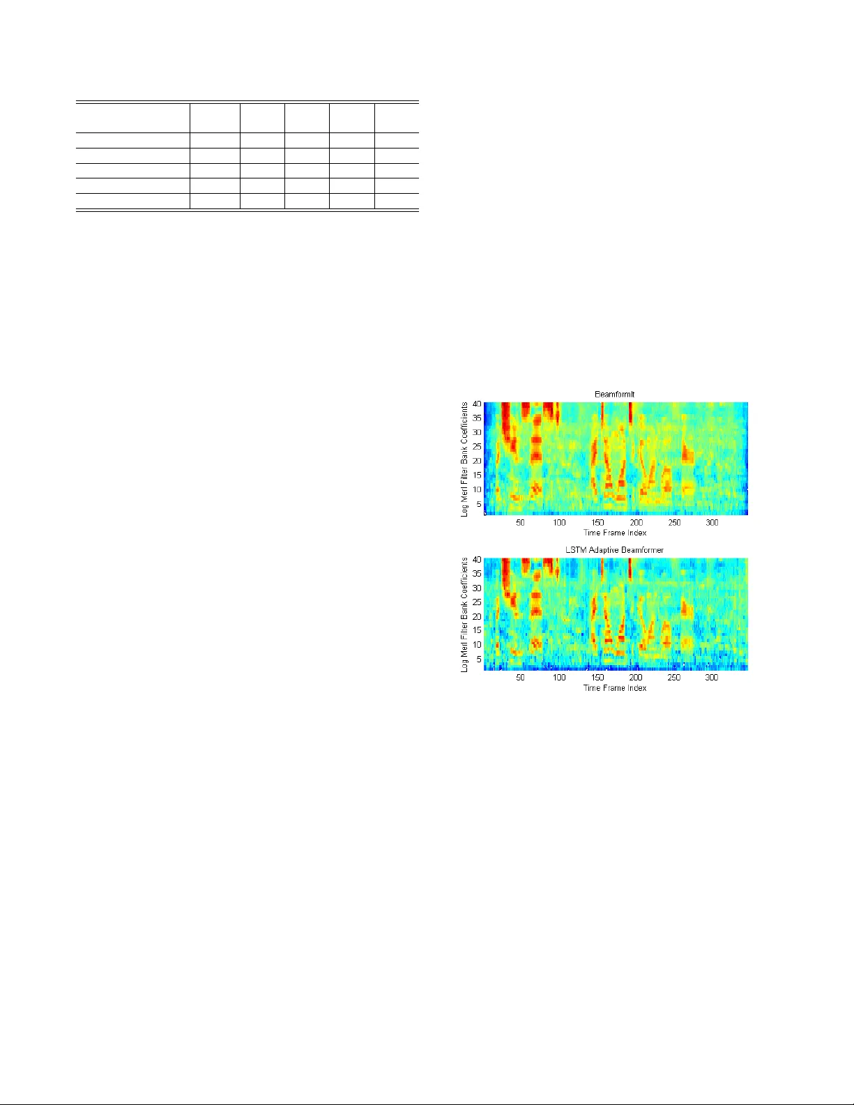
DEEP LONG SHOR T -TERM MEMOR Y AD APTIVE BEAMFORMING NETWORKS FOR MUL TICHANNEL R OBUST SPEECH RECOGNITION Zhong Meng 1 , 2 ∗ , Shinji W atanabe 1 , J ohn R. Hershe y 1 , Hakan Er dogan 3 1 Mitsubishi Electric Research Laboratories, Cambridge, MA 2 Georgia Institute of T echnology , Atlanta, GA 3 Microsoft Research, Redmond, W A ABSTRA CT Far -field speech recognition in noisy and reverberant conditions remains a challenging problem despite recent deep learning break- throughs. This problem is commonly addressed by acquiring a speech signal from multiple microphones and performing beam- forming ov er them. In this paper , we propose to use a recurrent neural network with long short-term memory (LSTM) architecture to adapti vely estimate real-time beamforming filter coefficients to cope with non-stationary environmental noise and dynamic nature of source and microphones positions which results in a set of time- varying room impulse responses. The LSTM adaptiv e beamformer is jointly trained with a deep LSTM acoustic model to predict senone labels. Further , we use hidden units in the deep LSTM acoustic model to assist in predicting the beamforming filter coef- ficients. The proposed system achieves 7.97% absolute gain ov er baseline systems with no beamforming on CHiME-3 real e valuation set. Index T erms — beamforming, multichannel, speech recogni- tion, LSTM 1. INTR ODUCTION Although extraordinary performance has been achieved in automatic speech recognition (ASR) with the advent of deep neural networks (DNNs) [1, 2], the performance still degrades dramatically in noisy and far-field situations [3, 4]. T o achie ve robust speech recognition, multiple microphones can be used to enhance the speech signal, re- duce the effects of noise and reverberation, and improv e the ASR performance. In this scenario, an essential step of the ASR front-end processing is multichannel filtering, or beamforming , which steers a spatial sensitivity region, or “beam, ” in the direction of the tar- get source, and inserts spatial suppression regions, or “nulls, ” in the directions corresponding to noise and other interference. Delay-and-sum (DAS) beamforming is widely used for multi- channel signal processing [5], in which the multichannel inputs of an microphone array are delayed to be aligned in time and then summed up to be a single channel signal. The signal from the tar get direction is enhanced and the noises and interferences coming from other di- rections are attenuated. Filter-and-sum beamforming applies filters to the input channels before summing them up [6]. Minimum vari- ance distortionless response (MVDR) [7] and generalized eigenv alue (GEV) [8] are filter -and-sum beamforming methods which solve for filter coefficients using dif ferent deriv ations. ∗ Zhong Meng performed the work while he was an intern at Mitsubishi Electric Research Laboratories, Cambridge, MA. Although these methods hav e achieved good performance in beamforming, their goal is to optimize only the signal-lev el objec- tiv e (e.g., SNR). In order to achieve robust speech recognition, it is more important to jointly optimize beamforming and acoustic model with the objectiv e of maximizing the ASR performance. In [9], the parameters of a frequency-domain beamformer are first estimated by a DNN based on the generalized cross correlation between microphones. Con ventional features are extracted from the beamformed signal before passing through a second DNN for acoustic modeling. Instead of filtering in the frequency domain, [10] performs spatial and spectral filtering through time-domain con volution over raw wa veform. The output feature is then passed to a con volutional LSTM DNN (CLDNN) acoustic model to predict the conte xt-dependent state output tar gets. In [11], the beamforming and frequency decomposition are factorized into separate layers in the network. These approaches assume that the speaker position and the en vironment are fixed and estimate constant filter coefficients for either beamforming or spatial and spectral filtering. Howe ver , in real noisy and far-field scenarios, as the position of the source (speaker), noise and room impulse response keep chang- ing, the time-in variant filter coefficients estimated by these neural networks may fail to robustly enhance the target signal. Therefore, we propose to adaptiv ely estimate the beamforming filter coefficients at each time frame using an LSTM to deal with an y possible changes of the source, noise or channel conditions. The enhanced signal is generated by applying these time-variant filter coef ficients to the short-time Fourier transform (STFT) of the array signals. Log filter- bank like features are obtained from the enhanced signal and then passed to a deep LSTM acoustic model to predict the senone pos- terior . The LSTM beamforming network and the LSTM acoustic model are jointly trained using truncated back-propagation through time (BPTT) with a cross-entropy objective. STFT coefficients of the array signals are used as the input of the beamforming network. In ASR systems of [12, 13], the speech signal is enhanced by NMF and LSTM before fed into the acoustic model. But speech enhance- ment module and the acoustic model are not jointly optimized to minimize the WER and the input is only single channel signal. Previous work [14] has shown that the speech separation per- formance can be improv ed by incorporating the speech recognition alignment information within the speech enhancement framew ork. Inspired by this, we feed the units of the top hidden layer of the LSTM acoustic model at the previous time step back as an auxil- iary input to the beamforming network to predict the current filter coefficients. Note that our work is different from [15] in that: (1) we perform adaptive beamforming over 5 different input channels, but their system works only on 2 input channels; (2) our adaptive LSTM beamformer predicts only the frequency domain filter coef- ficients and performs frequency domain filter-and-sum over STFT coefficients, while their work majorly focuses on the time-domain filtering with ra w wav eforms as the input; (3) the log Mel filter bank like features are generated with fixed log Mel transform over the beamformed STFT coefficients for acoustic modeling in our work, while time/frequency domain con volution is performed with train- able parameters on the beamformed features in their work; (4) no additional gate modulation is applied to the feedback to reduce the system complexity for our much smaller dataset. In the experi- ments, we show that this feedback captures high-level knowledge about the acoustic states and increases the performance. The exper - iments are conducted with the CHiME 3 dataset. The joint training of LSTM adaptiv e beamforming network and deep LSTM acoustic model achiev es 7.75% absolute gain over the single channel signal on the real test data. The acoustic model feedback provides an extra gain of 0.22%. 2. LSTM AD APTIVE BEAMFORMING 2.1. Adaptive Filter -and-Sum Beamforming As a generalization of the delay-and-sum beamforming, filter-and- sum beamformer processes the signal from each microphone using a finite impulse response (FIR) filter before summing them up. In frequency domain, this operation can be written as: ˆ x t,f = M X m =1 g f ,m x t,f ,m , (1) where x t,f ,m ∈ C is the complex STFT coefficient for the time- frequency index ( t, f ) of the signal from channel m , g f ,m ∈ C is the beamforming filter coefficient and ˆ x t,f ∈ C is the complex STFT coefficient of the enhanced signal. In Eq. (1), t = 1 , . . . , T , f = 1 , . . . , F and M , T , F are the numbers of microphones, time frames and frequencies. T o cope with the time-variant source position and room impulse response, we make the filter coefficients time- dependent and propose the adaptiv e filter-and-sum beamforming: ˆ x t,f = M X m =1 g t,f ,m x t,f ,m , (2) where g t,f ,m ∈ C is time-v ariant complex filter coefficient. 2.2. Adaptive LSTM Beamforming Network The LSTM network is a special kind of recurrent neural network (RNN) with purpose-built memory cells to store information [16]. The LSTM has been successfully applied to many different tasks [17, 18] due to its strong capability of learning long-term dependen- cies. The LSTM takes in an input sequence x = { x 1 , . . . , x T } and computes the hidden vector sequence h = { h 1 , . . . , h T } by iterat- ing the equation below h t = LSTM ( x t , h t − 1 ) (3) W e implement the LSTM in Eq. (3) with no peep hole connections. In this work, we apply r eal-value LSTM to the adaptive filter- and-sum beamformer to predict the real and imaginary parts of the complex filter coefficients at time t and channel m . That is, we introduce the following real-value v ectors for complex values g t,f ,m and x t,f ,m in Eq. (2): g t,m , [ < ( g t,f ,m ) , = ( g t,f ,m )] F f =1 ∈ R 2 F x t , [ < ( x t,f ,m ) , = ( x t,f ,m )] F,M f =1 ,m =1 ∈ R 2 F M . W ith this representation, the real-value LSTM predicts g t,m as fol- lows: p t = W x,p x t (4) h t = LSTM B F ( p t , h t − 1 ) (5) g t,m = tanh( W h,m h t ) , m = 1 , . . . , M , (6) where W x,p and W h,m are projection matrices. W e use tanh( · ) function to limit the range of the filter coefficients within [ − 1 , 1] . The real and imaginary parts of the STFT coef ficient ˆ x t,f of the beamformed signal are generated by Eq. (2) as follows ( < ( ˆ x t,f ) = P M m =1 < ( x t,f ,m ) < ( g t,f ,m ) − = ( x t,f ,m ) = ( g t,f ,m ) = ( ˆ x t,f ) = P M m =1 < ( x t,f ,m ) = ( g t,f ,m ) + = ( x t,f ,m ) < ( g t,f ,m ) . (7) More sophisticated features can be extracted from the beamformed STFT coefficients and are passed to the LSTM acoustic model to predict the senone posterior . In our e xperiments, the log Mel filter - bank like feature is generated from Eq. (7) by z t = log ( Mel ( P t )) (8) P t =  < ( ˆ x t,f ) 2 + = ( ˆ x t,f ) 2  F f =1 ∈ R F (9) where Mel ( · ) is the operation of Mel matrix multiplication, and P t is F dimensional real-v alue vector of the po wer spectrum of the beam- formed signal at time t . Global mean and variance normalization is applied to this log Mel filterbank like feature. Note that all op- erations in this section are performed with the r eal-value computa- tion, and can be easily represented by a dif ferentiable computational graph. 2.3. Deep LSTM Acoustic Model Recently , LSTMs are shown to be more effecti ve than DNNs [1, 2] and con ventional RNNs [19, 20] for acoustic modeling as they are able to model temporal sequences and long-range dependen- cies more accurately than the others especially when the amount of training data is large. LSTM has been successfully applied in both the RNN-HMM hybrid systems [21, 22] and the end-to-end system [23, 24]. In this work, the deep LSTM-HMM hybrid system is utilized for acoustic modeling. A forced alignment is first generated by a GMM-HMM system and is then used as the frame-lev el acoustic tar- gets which the LSTM attempts to classify . The LSTM is trained with cross-entropy objecti ve function using truncated BPTT . In this paper, to connect the deep LSTM with the adapti ve LSTM beamformer , we compute log Mel filterbank z t from the beamformed STFT coeffi- cients. q t = W z,p z t (10) s t = LSTM AM ( q t , s t − 1 ) (11) y t = softmax ( W s,y s t ) (12) q t is the projection of z t into a high-dimensional space and y t is the senone posterior . 2.4. Integrated Network of LSTM Adaptive Beamformer and Deep LSTM Acoustic Model In order to achiev e robust speech recognition by making use of mul- tichannel speech signals, LSTM beamformer in Section 2.2 and the deep LSTM acoustic model in Section 2.3 need to be jointly opti- mized with the objective of maximizing the ASR performance. In other words, the beamforming LSTM needs to be concatenated with the LSTM acoustic model to form an integrated network that takes multichannel STFT coefficients as the input and produces senone posteriors as illustrated in Fig. 1. The deep LSTM has three hidden layers in our experiments b ut only one is shown here for simplicity . T o train the integrated LSTM network, we connect the beam- forming network (2) – (6), log Mel filtering (8), and the acoustic model (10) – (12) as a single feed forward network, and back- propagate the gradient of the cross-entropy objectiv e function through the network so that both the adaptive beamformer and the acoustic model are optimized for the ASR task by using multi- channel training data. Fig. 1 . The unfolded integrated network of an LSTM adapti ve beam- former and an LSTM acoustic model. The acoustic feedback (in blue) is introduced to allo w the hidden units in LSTM acoustic model to assist in predicting the filter coefficient at current time. On top of that, we feed the hidden units of the top hidden layer of the deep LSTM acoustic model back to the input of the LSTM beamformer as the auxiliary feature to predict the filter coef ficients at next time. By introducing the acoustic model feedback, the Eq. (5) is re-written as h t = LSTM B F (( p t , s t − 1 ) , h t − 1 ) (13) where ( p t , s t − 1 ) is the concatenation of the acoustic feedback from previous time s t − 1 and the current projection p t . Direct training of the integrated network easily falls into a lo- cal optimum as the gradients for the LSTM beamformer and the deep LSTM acoustic model have different dynamic ranges. For a robust estimation of the model parameters, the training should be performed in sequence as shown in Algorithm 1. 3. EXPERIMENTS 3.1. CHiME-3 Dataset The CHiME-3 dataset is released with the 3rd CHiME speech Sepa- ration and Recognition Challenge [25], which incorporates the W all Street Journal corpus sentences spoken by talkers situated in chal- lenging noisy en vironment recorded using a 6-channel tablet based Algorithm 1 T rain LSTM adaptive beamformer and deep LSTM acoustic model 1: T rain a deep LSTM acoustic model with log Mel filterbank fea- ture extracted from the speech of all channels to minimize the cross-entropy objecti ve. 2: Initialize the integrated network with the deep LSTM acoustic model in Step 1. 3: T rain the integrated network with the ASR cross-entropy objec- tiv e, update only the parameters in the LSTM beamformer . 4: Jointly train the integrated network in Step 3 with the ASR cross-entropy objective, updating all parameters in the LSTM beamformer and deep LSTM acoustic model. 5: Introduce the acoustic feedback and re-train the integrated net- work with the ASR objecti ve, updating all the parameters. microphone array . CHiME-3 dataset consists of both real and simu- lated data. The real data is recorded speech spoken by actual talkers in four real noisy environments (on buses, in caf ´ es, in pedestrian areas, and at street junctions). T o generate the simulated data, the clean speech is first con voluted with the estimated impulse response of the en vironment and then mix ed with the background noise sep- arately recorded in that en vironment [4]. The training set consists of 1600 real noisy utterances from 4 speakers, and 7138 simulated noisy utterances from the 83 speakers in the WSJ0 SI-84 training set recorded in 4 noisy en vironments. There are 3280 utterances in the dev elopment set including 410 real and 410 simulated utterances for each of the 4 environments. There are 2640 utterances in the test set including 330 real and 330 simulated utterances for each of the 4 environments. The speakers in training set, dev elopment set and the test set are mutually different (i.e., 12 different speakers in the CHiME-3 dataset). The training, dev elopment and test data are all recorded in 6 different channels. The WSJ0 text corpus is also used to train the language model. 3.2. Baseline System The baseline system is built with Chainer [26] and Kaldi [27] toolk- its. 40-dimensional log Mel filterbank features extracted by Kaldi from all 6 channels are used to train a deep LSTM acoustic model us- ing Chainer . The LSTM has 3 layers and each hidden layer has 1024 units. The output layer has 1985 units, each of which corresponds to a senone tar get. The input feature is first projected to a 1024 di- mensional space before being fed into the LSTM. The forced align- ment generated by a GMM-HMM system trained with data from all 6 channels is used as the tar get for LSTM training. During e valua- tion, only the de velopment and test data from the 5 th channel is used for testing (only for the baseline system). The LSTM is trained using BPTT with a truncation size of 100 and a learning rate of 0 . 01 . The batch size for stochastic gradient descent (SGD) is 100. The WER performance of the baseline system is shown in T able 1. 3.3. LSTM Adaptive Beamformer The 257-dimensional complex STFT coefficients are extracted for the speech in channels 1 , 3 , 4 , 5 , 6 . The real and imaginary parts of STFT coefficients from all the 5 channels are concatenated together to form 257 × 2 × 5 = 2570 dimensional input of the beamform- ing LSTM. The input is projected to 1024 dimensional space before being fed into the LSTM. The beamforming LSTM has one hidden layer with 1024 units. The hidden units vector is projected to 5 sets of 257 × 2 = 514 dimensional filter coefficients for adaptiv ely beam- System Input Feature Simu Dev Real Dev Simu T est Real T est AM (baseline) Fbank 16.15 19.24 23.02 32.88 BeamformIt+AM STFT 14.32 12.99 24.36 21.21 BF+AM (fixed) STFT 15.23 15.01 23.14 25.64 BF+AM STFT 14.43 15.19 22.40 25.13 BF+AM+Feedback STFT 14.28 15.10 22.23 24.91 T able 1 . The WER performance (%) of the baseline LSTM acous- tic model (AM), BeamformIt-enhanced signal as the input of the AM, joint training of LSTM beamformer and LSTM acoustic model (BF+AM) with or without acoustic feedback. forming signals from 5 channels using Eq. (2). The MSE objecti ve is computed between the beamformed signal and BeamformIt [28]. The beamforming LSTM is trained using BPTT with a truncation size of 100 , a batch size of 100 and a learning rate of 1 . 0 . 3.4. Joint T raining of the Integrated Network The baseline LSTM acoustic model trained in Section 3.2 and the LSTM adaptiv e beamformer trained in Section 3.3 are concatenated together as the initialization of the integrated network. A feature extraction layer is inserted in between the two LSTMs to extract 40- dimensional log Mel filterbank features with Eq. (8). The integrated network is trained in a way described in Steps 3, 4 and 5 of Section 2.4. BPTT with a truncation size of 100 and a batch size of 100 and a learning rate of 0 . 01 is used for training. The data from all 5 channels in the development and test set is used for ev aluating the integrated network. The WER performance for different cases are shown in T able 1. 3.5. Result Analysis From T able 1, the best system is the integrated network of an LSTM adaptiv e beamformer and a deep LSTM acoustic model with the acoustic feedback, which achiev es 14.28%, 15.10%, 22.23%, 24.91% WERs on the simulated dev elopment set, real development set, simulated test set and real test set of the CHiME-3 dataset respectiv ely . The joint training of the integrated network without updating the deep LSTM acoustic model achie ves absolute gains of 0.92%, 4.23% and 7.24% ov er the baseline system on the simulated dev elopment set, real development set and real test set respectiv ely . The joint training of the inte grated network with all the parameters updated achie ves absolute gains of 1.72%, 4.05%, 0.62% and 7.75% respectiv ely ov er the baseline systems on the simulated dev elop- ment set, real dev elopment set, simulated test set and real test set respectiv ely . The large performance improvement justifies that the LSTM adaptive beamformer is able to estimate the real-time filter coefficients adapti vely in response to the changing source position, en vironmental noise and room impulse response with the LSTM acoustic model jointly trained to optimize the ASR objective. Fur- ther absolute gains of 0.15%, 0.09%, 0.17% and 0.22% are achieved with the introduction of acoustic feedback, which indicates that the high-lev el acoustic information is also helpful in predicting the filter coefficients at the ne xt time step. Note that although the proposed system with acoustic feedback achiev es 0.04% and 2.13% absolute gains o ver the beamformed sig- nal generated by BeamformIt on the simulated de velopment and test sets, it does not work as well as the BeamformIt on the real de velop- ment and test sets. In BeamformIt implementation, the two-step time delay of arriv al V iterbi postprocessing makes use of both the past and future information in predicting the best alignment of multiple chan- nels at the current time, while in our system, only the history in the past is utilized to estimate the current filter coefficients. This may explain the differences in WER performance and can be alleviated by using bidirectional LSTM as part of the future work. 3.6. Beamformed Featur e The LSTM beamformer adaptiv ely predicts the time-variant beam- forming coefficients and performs filter-and-sum beamforming ov er the 5 input channels. The log Mel filter bank feature is obtained from the STFT coefficients. From Fig. 2, we see that the log Mel filter bank feature obtained from the LSTM adaptive beamformer is quite similar to the log Mel filter bank feature extracted from the STFT coefficients beamformed by BeamformIt for the same utter- ance. The SNR is not high but matches the LSTM acoustic model well for maximizing the ASR performance. Fig. 2 . The comparison of the log Mel filter bank coefficients of the same utterance extracted from STFT coef ficients beamformed by BeamformIt (upper) and LSTM adaptiv e beamformer (lower) . 4. CONCLUSIONS In this work, LSTM adapti ve beamforming is proposed to adaptively predict the real-time beamforming filter coefficients to deal with the time-variant source location, en vironmental noise and room impulse response inherent in the multichannel speech signal. T o achie ve ro- bust ASR, the LSTM adaptiv e beamformer is jointly trained with a deep LSTM acoustic model to optimize the ASR objectiv e. This framew ork achiev es absolute gains of 1.72%, 4.05%, 0.62% and 7.75% over the baseline system on the CHiME-3 dataset. Further improv ement is achie ved by introducing the acoustic feedback to as- sist in predicting the filter coefficients. Howe ver , our approach does not work as well as the BeamformIt on real data and we will look into this in the future. 5. REFERENCES [1] G. Hinton, L. Deng, D. Y u, G. E. Dahl, A. r . Mohamed, N. Jaitly , A. Senior , V . V anhoucke, P . Nguyen, T . N. Sainath, and B. Kingsbury , “Deep neural networks for acoustic model- ing in speech recognition: The shared views of four research groups, ” IEEE Signal Pr ocessing Magazine , vol. 29, no. 6, pp. 82–97, Nov 2012. [2] G. E. Dahl, D. Y u, L. Deng, and A. Acero, “Context-dependent pre-trained deep neural networks for large-vocab ulary speech recognition, ” IEEE T ransactions on Audio, Speech, and Lan- guage Pr ocessing , vol. 20, no. 1, pp. 30–42, Jan 2012. [3] Marc Delcroix, T akuya Y oshioka, Atsunori Ogawa, Y otaro Kubo, Masakiyo Fujimoto, Nobutaka Ito, Keisuke Kinoshita, Miquel Espi, Shoko Araki, T akaaki Hori, and T omohiro Nakatani, “Strategies for distant speech recognitionin reverber - ant en vironments, ” EURASIP Journal on Advances in Signal Pr ocessing , vol. 2015, no. 1, pp. 1–15, 2015. [4] T . Hori, Z. Chen, H. Erdogan, J. R. Hershey , J. Le Roux, V . Mi- tra, and S. W atanabe, “The merl/sri system for the 3rd chime challenge using beamforming, robust feature extraction, and advanced speech recognition, ” in 2015 IEEE W orkshop on Au- tomatic Speech Recognition and Understanding (ASR U) , Dec 2015, pp. 475–481. [5] Jacob Benesty , Jingdong Chen, and Y iteng Huang, Micro- phone array signal pr ocessing , vol. 1, Springer Science & Business Media, 2008. [6] Barry D V an V een and Kevin M Buckley , “Beamforming: A versatile approach to spatial filtering, ” IEEE assp magazine , vol. 5, no. 2, pp. 4–24, 1988. [7] H Erdogan, JR Hershey , S W atanabe, M Mandel, and J Le Roux, “Impro ved mvdr beamforming using single- channel mask prediction networks, ” 2016. [8] E. W arsitz and R. Haeb-Umbach, “Blind acoustic beamform- ing based on generalized eigen value decomposition, ” IEEE T ransactions on Audio, Speech, and Language Processing , vol. 15, no. 5, pp. 1529–1539, July 2007. [9] X. Xiao, S. W atanabe, H. Erdogan, L. Lu, J. Hershey , M. L. Seltzer , G. Chen, Y . Zhang, M. Mandel, and D. Y u, “Deep beamforming networks for multi-channel speech recognition, ” in 2016 IEEE International Conference on Acoustics, Speech and Signal Pr ocessing (ICASSP) , March 2016, pp. 5745–5749. [10] T . N. Sainath, R. J. W eiss, K. W . Wilson, A. Narayanan, M. Bacchiani, and Andre w , “Speaker location and microphone spacing in variant acoustic modeling from raw multichannel wa veforms, ” in 2015 IEEE W orkshop on Automatic Speech Recognition and Understanding (ASR U) , Dec 2015, pp. 30–36. [11] T . N. Sainath, R. J. W eiss, K. W . W ilson, A. Narayanan, and M. Bacchiani, “Factored spatial and spectral multichannel raw wa veform cldnns, ” in 2016 IEEE International Conference on Acoustics, Speec h and Signal Pr ocessing (ICASSP) , March 2016, pp. 5075–5079. [12] J. T . Geiger, F . W eninger , J. F . Gemmeke, M. Wllmer, B. Schuller , and G. Rigoll, “Memory-enhanced neural net- works and nmf for robust asr, ” IEEE/A CM T ransactions on Audio, Speech, and Language Pr ocessing , vol. 22, no. 6, pp. 1037–1046, June 2014. [13] Felix W eninger , Jrgen Geiger , Martin Wllmer , Bjrn Schuller, and Gerhard Rigoll, “Feature enhancement by deep { LSTM } networks for { ASR } in reverberant multisource environ- ments, ” Computer Speech & Language , vol. 28, no. 4, pp. 888 – 902, 2014. [14] H. Erdogan, J. R. Hershey , S. W atanabe, and J. Le Roux, “Phase-sensitiv e and recognition-boosted speech separation using deep recurrent neural networks, ” in 2015 IEEE Interna- tional Conference on Acoustics, Speech and Signal Pr ocessing (ICASSP) , April 2015, pp. 708–712. [15] Bo Li, T ara N Sainath, Ron J W eiss, Kevin W Wilson, and Michiel Bacchiani, “Neural netw ork adaptiv e beamforming for robust multichannel speech recognition, ” in Pr oc. Interspeech , 2016. [16] S. Hochreiter and J. Schmidhuber , “Long short-term memory , ” Neural Computation , vol. 9, no. 8, pp. 1735–1780, Nov 1997. [17] A. Grav es, A. r . Mohamed, and G. Hinton, “Speech recognition with deep recurrent neural networks, ” in 2013 IEEE Interna- tional Conference on Acoustics, Speech and Signal Pr ocessing , May 2013, pp. 6645–6649. [18] Martin Sundermeyer , Ralf Schl ¨ uter , and Hermann Ney , “Lstm neural networks for language modeling., ” in Interspeech , 2012, pp. 194–197. [19] C. W eng, D. Y u, S. W atanabe, and B. H. F . Juang, “Recur- rent deep neural networks for robust speech recognition, ” in 2014 IEEE International Conference on Acoustics, Speech and Signal Pr ocessing (ICASSP) , May 2014, pp. 5532–5536. [20] O. V inyals, S. V . Ravuri, and D. Povey , “Re visiting recur- rent neural networks for robust asr, ” in 2012 IEEE Interna- tional Conference on Acoustics, Speech and Signal Pr ocessing (ICASSP) , March 2012, pp. 4085–4088. [21] A. Graves, N. Jaitly , and A. r . Mohamed, “Hybrid speech recognition with deep bidirectional lstm, ” in A utomatic Speech Recognition and Understanding (ASR U), 2013 IEEE W orkshop on , Dec 2013, pp. 273–278. [22] Hasim Sak, Andre w W Senior , and Franc ¸ oise Beaufays, “Long short-term memory recurrent neural network architectures for large scale acoustic modeling., ” in INTERSPEECH , 2014, pp. 338–342. [23] A. Grav es, A. r . Mohamed, and G. Hinton, “Speech recognition with deep recurrent neural networks, ” in 2013 IEEE Interna- tional Conference on Acoustics, Speech and Signal Pr ocessing , May 2013, pp. 6645–6649. [24] Jan K Chorowski, Dzmitry Bahdanau, Dmitriy Serdyuk, Kyungh yun Cho, and Y oshua Bengio, “ Attention-based mod- els for speech recognition, ” in Advances in Neural Information Pr ocessing Systems , 2015, pp. 577–585. [25] J. Barker , R. Marxer , E. V incent, and S. W atanabe, “The third chime speech separation and recognition challenge: Dataset, task and baselines, ” in 2015 IEEE W orkshop on Automatic Speech Recognition and Understanding (ASR U) , Dec 2015, pp. 504–511. [26] Seiya T okui, K enta Oono, Shohei Hido, and Justin Clayton, “Chainer: a next-generation open source framew ork for deep learning, ” in Pr oceedings of W orkshop on Machine Learning Systems (LearningSys) in The T wenty-ninth Annual Conference on Neural Information Pr ocessing Systems (NIPS) , 2015. [27] Daniel Povey , Arnab Ghoshal, Gilles Boulianne, Lukas Bur- get, Ondrej Glembek, Nagendra Goel, Mirko Hannemann, Petr Motlicek, Y anmin Qian, Petr Schwarz, Jan Silovsky , Georg Stemmer , and Karel V esely , “The kaldi speech recognition toolkit, ” in IEEE 2011 W orkshop on Automatic Speech Recog- nition and Understanding . Dec. 2011, IEEE Signal Processing Society , IEEE Catalog No.: CFP11SR W -USB. [28] X. Anguera, C. W ooters, and J. Hernando, “ Acoustic beam- forming for speaker diarization of meetings, ” IEEE T ransac- tions on Audio, Speech, and Language Processing , vol. 15, no. 7, pp. 2011–2022, Sept 2007.