Deep Reinforcement Learning for Time Scheduling in RF-Powered Backscatter Cognitive Radio Networks

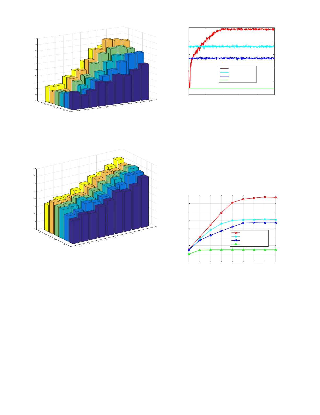
Deep Reinforcement Learning for T ime Scheduling in RF-Po wered Backscatter Cogniti v e Radio Networks T ran The Anh 1 , Nguyen Cong Luong 1 , Dusit Niyato 1 , Y ing-Chang Liang 2 , and Dong In Kim 3 1 School of Computer Science and Engineering, Nanyang T echnological Uni versity , Singapore 2 Center for Intelligent Networking and Communications, Uni versity of Electronic Science and T echnology of China, China 3 School of Information and Communication Engineering, Sungkyunkwan Uni versity , Korea Abstract —In an RF-powered backscatter cognitive radio net- work, multiple secondary users communicate with a secondary gateway by backscattering or harvesting ener gy and actively transmitting their data depending on the primary channel state. T o coordinate the transmission of multiple secondary transmit- ters, the secondary gateway needs to schedule the backscattering time, energy harvesting time, and transmission time among them. Howev er , under the dynamics of the primary channel and the uncertainty of the energy state of the secondary transmitters, it is challenging for the gateway to find a time scheduling mechanism which maximizes the total throughput. In this paper , we propose to use the deep reinf orcement learning algorithm to derive an optimal time scheduling policy for the gateway . Specifically , to deal with the pr oblem with large state and action spaces, we adopt a Double Deep-Q Network (DDQN) that enables the gateway to learn the optimal policy . The simulation results clearly show that the proposed deep reinf orcement learning algorithm outperforms non-learning schemes in terms of network throughput. Index T erms —Cognitive radio networks, ambient backscatter , RF energy harvesting, time scheduling, deep reinf orcement learn- ing. I . I N T RO D U C T I O N Radio Frequency (RF)-po wered cogniti ve radio netw orks are considered to be a promising solution which improves radio spectrum utilization and efficienc y as well as addresses the energy constraint issue for lo w-power secondary systems, e.g., the IoT system [1], [2], [3]. Howe ver , in the RF-powered cognitiv e radio networks, RF-powered secondary transmitters typically require a long time period to harvest suf ficient energy for their activ e transmissions. This may significantly deteriorate the network performance. Thus, RF-powered cog- nitiv e radio networks with ambient backscatter [4] have been recently proposed. In the RF-powered backscatter cognitiv e radio network, a primary transmitter, e.g., a base station, transmits RF signals on a licensed channel. When the channel is busy , the secondary transmitters either transmit their data to a secondary gate way by using backscatter communications or harvest energy from the RF signals through RF energy harvesting techniques. When the channel is idle, the secondary transmitters use the harvested ener gy to transmit their data to the gateway . As such, the RF-powered backscatter cognitiv e radio network enables secondary systems to simultaneously optimize the spectrum usage and energy harvesting to maxi- mize their performance. Howe ver , one major problem in the RF-powered backscatter cognitiv e radio network is how the secondary gate way 1 schedules the backscattering time, energy harvesting time, and transmission time among multiple sec- ondary transmitters so as to maximize the network throughput. T o address the problem, optimization methods and game theory can be used. The authors in [5] optimized the time scheduling for the gatew ay in the RF-powered backscatter cognitiv e radio network through using the Stackelberg game. In the game, the gatew ay is the leader , and the secondary transmitters are the followers. The gatew ay first determines spectrum sensing time and an interference price to maximize its rev enue. Based on the time and price, each secondary trans- mitter determines the energy harvesting time, backscattering time, and transmission time so as to maximize its throughput. Howe ver , the proposed game requires complete and perfect sensing probability information, and thus the game cannot deal with the dynamics of the network en vironment. T o optimize the performance of RF powered backscatter cognitiv e radio in the dynamic en vironment and with large state and action space, deep reinforcement learning (DRL) technique [6] can be adopted. In principle, the DRL im- plements a Deep Q-Network (DQN), i.e., the combination of a deep neural network and the Q-learning, to deriv e an approximate v alue of Q-values of actions, i.e., decisions. Compared with the conv entional reinforcement learning, the DRL can improve significantly the learning performance and the learning speed. Therefore, in this paper, we propose to use the DRL for the time scheduling in the RF-powered backscatter cognitiv e radio network. In particular, we first formulate a stochastic optimization problem that maximizes the total throughput for the network. The DRL algorithm is adopted to achieve the optimal time scheduling policy for the secondary transmitters. T o ov ercome the instability of the learning and to reduce the ov erestimation of action values, the Double DQN (DDQN) is used to implement the DRL algorithm. Simulation results show that the proposed DRL algorithm always achiev es the better performance compared with non-learning algorithms. T o the best of our knowledge, this is the first paper that inv estigates an application of DRL in the RF-powered backscatter cognitive radio network. The rest of this paper is organized as follows. Section II revie ws related work. Section III describes the system model and problem formulation. Section IV presents the DRL algo- 1 W e use “secondary gate way” and “gate way” interchangeably in the paper . rithm for the time scheduling in the RF-powered backscatter cognitiv e radio network. Section V shows the performance ev aluation results. Section VI summarizes the paper . I I . R E L A T E D W O R K Backscatter communications systems can be optimized to achiev e optimal throughput. In [7], the authors considered the data scheduling and admission control problem of a backscatter sensor network. The authors formulated the prob- lem as a Markov decision process, and learning algorithm was applied to obtain the optimal policy that minimizes the weighted sum of delay of different types of data. In [8], the authors formulated an optimization problem for ambient backscatter communications networks. The problem aims to deriv e an optimal control policy for sleep and active mode switching and reflection coefficient used in the active mode. Howe ver , only single transmitter was considered. In [9], the authors extended the study in [8] to a cognitiv e radio network. Specifically , the hybrid HTT and backscatter communications are adopted and integrated for a secondary user . The authors proposed an optimal time allocation scheme which is based on the conv ex optimization problem. While multiple secondary users were considered, the secondary user does not employ energy storage. The authors in [10] analyzed the backscatter wireless powered communication system with multiantenna by using the stochastic geometry approach. The energy and information outage probabilities in the energy harvesting and backscatter were deriv ed. Then, the authors introduced an optimization problem for time allocation to maximize ov erall network throughput. The authors in [11] introduced a two-way communication protocol for backscatter communications. The protocol combines time-switching and power splitting receiver structures with backscatter communication. The optimization problem was formulated and solved to maximize sum through- put of multiple nodes. Unlike the abov e works that consider time allocation, the authors in [12] proposed a channel-aware rate adaptation protocol for backscatter networks. The protocol first probes the channel and adjusts the transmission rate of the backscatter transmitter . The objective is to minimize the number of channels to be used for successfully communicating with all backscatter nodes. Although a fe w works in the literature studied the per- formance optimization of backscatter-based communications networks, almost all of them assume that information about the network is always av ailable which may not be realistic under random and unpredictable wireless environments. Therefore, this paper considers a scenario in which the network does not have complete information. The network needs to learn to assign backscattering time, energy harvesting time, and transmission time to the secondary transmitters to maximize the total network throughput. I I I . S Y S T E M M O D E L W e consider the RF-powered backscatter cognitiv e radio network. The network consists of a primary transmitter and N secondary transmitters (Fig. 1). The primary transmitter E n e rg y s t o ra g e D a t a q u e u e P a c k a g e a r ri v a l S e c o n d a ry t ra n s m i t t e r P ri m a ry t ra n s m i t t e r P ri m a ry s i g n a l E n e rg y s t o ra g e H a rv e s t i n g D a t a q u e u e S e c o n d a ry t ra n s m i t t e r G a t e w a y ( a g e n t ) Ba c k s c a t t e r T ra n s m i t Fig. 1. Ambient backscatter model with multiple secondary transmitters. F ra m e t () t  () n t  () n t  () bt () F b t  F ra m e t + 1 F ra m e t - 1 Fig. 2. Structure of frame t and time scheduling. transmits RF signal on a licensed channel. The transmission is organized into frames, and each frame is composed of F time slots. In Frame t (see Fig. 2), the transmission duration of the primary transmitter or the busy channel period, i.e., the number of time slots the channel is busy , is denoted by b ( t ) which is random. The secondary transmitters transmit data to the gate way . The gateway also controls the transmission scheduling of the secondary transmitters. In particular , during the busy channel period, the time slots can be assigned for energy harvesting by all the secondary transmitters. The number of time slots for energy harvesting is denoted by µ ( t ) . Let e h n denote the number of energy units that secondary transmitter n harvests in one busy time slot. The harvested energy is stored in energy storage, e.g., a super-capacitor , of the secondary transmitter , the maximum capacity of which is denoted by C n . A secondary transmitter has a data queue which stores an incoming packet, e.g., from its sensor device. The maximum capacity of the data queue is denoted by Q n , and the probability that a packet arrives at the queue in a time slot is denoted by λ n . Then, the rest of the busy time slots, i.e., b ( t ) − µ ( t ) , will be allocated for the secondary transmitters to transmit their data by using backscatter communications, i.e., the backscatter mode . The number of time slots for backscatter transmission by secondary transmitter n is denoted by α n ( t ) , and the number of packets transmitted in each time slot is d b n . Then, during the idle channel period which has F − b ( t ) time slots, the secondary transmitters can transfer data to the gate way by using active-RF transmission, i.e., the active mode . The number of time slots for secondary transmitter n to transmit in the activ e mode is denoted by β n ( t ) . Each time slot 2 can be used to transmit d a n packets from the data queue, and the secondary transmitter consumes e a n units of energy from the storage. The data transmission in the backscatter mode and in the activ e mode is successful with the probabilities S b n and S a n , respectively . Hence, the total throughput of the RF- powered backscatter cognitiv e radio network is the sum of the number of packets successfully transmitted by all secondary transmitters. I V . P RO B L E M F O R M U L A T I O N T o optimize the total throughput, we formulate a stochastic optimization problem for the RF-powered backscatter cog- nitiv e radio network. The problem is defined by a tuple < S , A , P , R > . • S is the state space of the network. • A is the action space. • P is the state transition probability function, where P s,s 0 ( a ) is the probability that the current state s ∈ S transits to the next state s 0 ∈ S when action a ∈ A is taken. • R is the reward function of the network. The state space of secondary transmitter n is denoted by S n = n ( q n , c n ); q n ∈ { 0 , 1 , . . . , Q n } , c n ∈ { 0 , 1 , . . . , C n } o , (1) where q n represents the queue state, i.e., the number of packets in the data queue, and c n represents the energy state, i.e., the number of energy units in the energy storage. Let the channel state, i.e., the number of b usy time slots, be denoted by S c = { ( b ); b ∈ { 0 , 1 , . . . , F }} . Then, the state space of the network is defined by S = S c × N Y n =1 S n , (2) where × and Q represent the Cartesian product. The action space of the network is defined as follo ws: A = ( ( µ, α 1 , . . . , α N , β 1 , . . . , β N ); µ + N X n =1 α n ≤ b, µ + N X n =1 ( α n + β n ) ≤ F ) , (3) where again µ is the number of busy time slots that are used for energy harvesting by the secondary transmitters, α n is the number of busy time slots that secondary transmitter n transmits data in the backscatter mode, and β n is the number of idle time slots that secondary transmitters n transmits data in the active mode. The constraint µ + P N n =1 α n ≤ b ensures that the number of time slots for energy harvesting and all backscatter transmissions do not exceed the number of busy time slots. Like wise, the constraint µ + P N n =1 ( α n + β n ) ≤ F ensures that the number of time slots for energy harvesting, all transmissions in the backscatter and active modes do not exceed the total number of time slots in a frame. Now , we consider the state transition of the network. In the busy channel period, the number of time slots assigned to secondary transmitter n for harvesting energy is b ( t ) − α n . Thus, after the busy channel period, the number of energy units in the storage of the secondary transmitter changes from c n to c (1) n as follows: c (1) n = min  c n + ( b ( t ) − α n ) e h n , C n  . (4) Also, the number of packets in the data queue of secondary transmitter n changes from q n to q (1) n as follows: q (1) n = max  0 , q n − α n d b n  . (5) In the idle channel period, secondary transmitter n requires q (1) n /d a n time slots to transmit q (1) n packets. Howe ver , the secondary transmitter is only assigned with β n time slots for the data transmission. Thus, it actually transmits its packets in min( β n , q (1) n /d a n ) time slots. After the idle channel period, the energy state of secondary transmitter n changes from c (1) n to c 0 n as follows: c 0 n = max  0 , c (1) n − min( β n , q (1) n /d a n ) e a n  . (6) Also, the number of packets in the data queue of secondary transmitter n changes from q (1) n to q (2) n as follows: q (2) n = max  0 , q (1) n − min( β n , c (1) n /e a n ) d a n  . (7) Note that new packets can arri ve at each time slot with a probability of λ n . W e assume that the new packets are only added to the data queue when the time frame finishes. Thus, at the end of the time frame, the number of packets in the data queue of secondary transmitter n changes from q (2) n to q 0 n as follows: q 0 n = q (2) n + p n , (8) where p n is the number of packets arriving in the secondary transmitter during the time frame. p n typically follows bino- mial distribution B ( F , λ n ) [13]. Then, the probability of m packets arri ving in the secondary transmitter during F time slots is P r ( p n = m ) =  F m  λ m n (1 − λ n ) F − m . (9) The re ward of the network is defined as a function of state s ∈ S and action a ∈ A as follows: R ( s, a ) = N X n =1 S b n ( q (1) n − q n ) + N X n =1 S a n ( q (2) n − q (1) n ) . (10) The first and the second terms of the reward expression in (10) are for the total numbers of packets transmitted in the backscatter and activ e modes, respecti vely . T o obtain the mapping from a network state s ∈ S to an action a ∈ A such that the accumulated rew ard is maximized, con ventional algorithm can be applied. The goal of the algorithm is to obtain the optimal policy defined as π ∗ : S → A . In the algorithm, the optimal policy to maximize value-state function is defined as follows: V ( s ) = E " T − 1 X t =0 γ t R ( s ( t ) , a ( t )) # , (11) 3 where T is the length of the time horizon, γ is the discount factor for 0 ≤ γ < 1 , and E [ · ] is the expectation. Here, we define a = π ( s ) which is the action taken at state s given the policy π . W ith the Markov property , the value function can be expressed as follo ws: V ( s ) = X s 0 ∈S P π ( s ) ( s, s 0 ) ( R ( s, a ) + γ V ( s 0 )) , (12) π ( s ) = max a ∈A X s 0 ∈S P π ( s ) ( s, s 0 )  R ( s, a ) + γ V ( s 0 )  ! . (13) W ith the Q-learning algorithm, Q-value is defined, and its optimum can be obtained from the Bellman’ s equation, which is giv en as Q ( s, a ) = X s 0 ∈S P π ( s ) ( s, s 0 ) ( R ( s, a ) + γ V ( s 0 )) . (14) The Q-value is updated as follows: Q new ( s, a ) =(1 − l ) Q ( s, a ) (15) + l  r ( s, a ) + γ max a 0 ∈A Q ( s 0 , a 0 )  . where l is the learning rate, and r ( s, a ) is the rew ard receiv ed. Howe ver , the standard algorithms and Q-learning to solve the stochastic optimization problem all suffer from lar ge state and action space of the networks. Thus, we resort to the deep reinforcement learning algorithm. V . D E E P R E I N F O R C E M E N T L E A R N I N G A L G O R I T H M By using (15) to update Q-values in a look-up table, the Q-learning algorithm can efficiently solve the optimization problem if the state and action spaces are small. In particular for our problem, the gate way needs to observe states of all N secondary transmitters and choose actions from their action spaces. As N grows, the state and action spaces can become intractably large, and sev eral Q-values in the table may not be updated. T o solve the issue, we propose to use a DRL algorithm. Similar to the Q-learning algorithm, the DRL allows the gate way to map its state to an optimal action. Howe ver , instead of using the look-up table, the DRL uses a Deep Q-Network (DQN), i.e., a multi-layer neural network with weights θ , to deriv e an approximate value of Q ∗ ( s, a ) . The input of the DQN is one of the states of the gate way , and the output includes Q-values Q ( s, a ; θ ) of all its possible actions. T o achiev e the approximate v alue Q ∗ ( s, a ) , the DQN needs to be trained by using transaction < s, a, r , s 0 > , i.e., experience, in which action a is selected through using the  -greedy policy . T raining the DQN is to update its weights θ to minimize a loss function defined as: L = E  ( y − Q ( s, a ; θ )) 2  , (16) where y is the target v alue. y is giv en by y = r + γ max a 0 ∈A Q ( s 0 , a 0 ; θ − ) , (17) where θ − are the old weights, i.e., the weights from the last iteration, of the DQN. Note that the max operator in (17) uses the same Q-values both to select and to ev aluate an action of the gate way . This means that the same Q-v alues are being used to decide which action is the best, i.e., the highest expected reward, and they are also being used to estimate the action v alue. Thus, the Q- value of the action may be over -optimistically estimated which reduces the network performance. T o prevent the overoptimism problem, the action selection should be decoupled from the action ev aluation [14]. There- fore, we use the Double DQN (DDQN). The DDQN includes two neural networks, i.e., an online network with weights θ and a target network with weights θ − . The target network is the same as the online network that its weights θ − are reset to θ of the online network e very L − iterations. At other iterations, the weights of the target network keep unchanged while those of the online network are updated at each iteration. In principle, the online network is trained by updating its weights θ to minimize the loss function as shown in (16). Howe ver , y is replaced by y DD QN defined as y DD QN = r + γ Q  s 0 , arg max a 0 ∈A Q i ( s 0 , a 0 ; θ ); θ −  . (18) As sho wn in (18), the action selection is based on the current weights θ , i.e., the weights of the online network. The weights θ − of the target network are used to fairly ev aluate the v alue of the action. The DDQN algorithm for the gateway to find its optimal policy is shown in Algorithm 1. Accordingly , both the online and target networks use the next state s 0 to compute the optimal value Q ( s 0 , a 0 ; θ ) . Giv en the discount factor γ and the current reward r , the target value y DD QN is obtained from (18). Then, the loss function is calculated as defined in (16) in which y is replaced by y DD QN . The value of the loss function is back propagated to the online network to update its weights θ . Note that to address the instability of the learning of the algorithm, we adopt an experience replay memory D along with the DDQN. As such, instead of using the most recent transition, a random mini-batch of transactions is taken from the replay memory to train the Q-network. V I . P E R F O R M A N C E E V A L UA T I O N In this section, we present experimental results to ev aluate the performance of the proposed DRL algorithm. For com- parison, we introduce the HTT [9], the backscatter commu- nication [4], and a random policy as baseline schemes. In particular for the random policy , the gate way assigns time slots to the secondary transmitters for the energy harvesting, data backscatter , and data transmission, by choosing randomly a tuple ( µ, α 1 , . . . , α N , β 1 , . . . , β N ) in action space A . Note that we do not introduce the reinforcement learning algorithm [1] since it cannot be run in our computation en vironment as the problem is too complex. The simulation parameters for the RF-powered backscatter cogniti ve radio network are sho wn in T able I, and those for the DRL algorithm are listed in T able II. 4 Algorithm 1 DDQN algorithm for time scheduling of the gate way . Input: Action space A ; mini-batch size L b ; target network replacement frequency L − . Output: Optimal policy π ∗ . 1: Initialize: Replay memory D ; online network weights θ ; tar- get network weights θ − = θ ; online action-value function Q ( s, a ; θ ) ; target action-value function Q ( s 0 , a 0 ; θ − ) ; k = i = 0 . 2: repeat for each episode i : 3: Initialize network state s after receiving state massages from the primary transmitter and N secondary transmitters. 4: repeat for each iteration k in episode i : 5: Choose action a according to  − g r eedy policy from Q ( s, a ; θ ) . 6: Broadcast time scheduling massages defined by a to N secondary transmitters. 7: Receiv e an immediate reward r k . 8: Receiv e state massages from primary transmitter and N secondary transmitters and update next network state s 0 . 9: Store tuple ( s, a, r k , s 0 ) in D . 10: Sample a mini-batch of L b tuples ( s, a, r t , s 0 ) from D . 11: Define a max = arg max a 0 ∈A Q ( s 0 , a 0 ; θ ) . 12: Determine y DD QN t = ( r t , if episode i terminates at iteration t + 1 , r t + γ Q  s 0 , a max ; θ −  , otherwise . 13: Update θ by performing a gradient descent step on ( y DD QN t − Q ( s, a ; θ )) 2 . 14: Reset θ − = θ ev ery L − steps. 15: Set s ← s 0 . 16: Set k = k + 1 . 17: until k is greater than the maximum number of steps in episode i . 18: Set i = i + 1 . 19: until i is greater than the desired number of episodes. The DRL algorithm is implemented by using the T ensorFlow deep learning library . The Adam optimizer is used that allows to adjust the learning rate during the training phase. The  - greedy policy with  = 0 . 9 is applied in the DRL algorithm to balance the e xploration and exploitation. This means that a random action is selected with a probability of  = 0 . 9 , and the best action, i.e., the action that maximizes the Q-value, is selected with a probability of  = 0 . 1 . T o move from a more explorati ve policy to a more exploitativ e one, the value of  is linearly reduced from 0 . 9 to 0 during the training phase. T o ev aluate the performance of the proposed DRL algo- rithm, we consider dif ferent scenarios by v arying the number of busy time slots per time frame, i.e., by v arying τ , and the packet arri val probability λ . The simulation results for the throughput versus episode are shown in Fig. 5, those for the throughput versus the packet arri val probability are illustrated in Fig. 6, and those for the throughput versus the number of busy time slots are provided in Fig. 7. Note that the throughput is the sum of the number of packets successfully transmitted by all secondary transmitters. In particular for the proposed DRL algorithm, the throughput T ABLE I B A CK S C A TT E R C O G N IT I V E R A DI O N E T W OR K PA R AM E T E RS P arameters V alue Number of secondary transmitters ( N ) 3 Number of time slots in a time frame ( F ) 10 Number of idle time slots in a time frame ( b ( t ) ) [1;9] Data queue size ( Q n ) 10 Energy storage capacity ( C n ) 10 Packet arriv al probability ( λ n ) [0.1;0.9] d b n 1 d a n 2 e h n 1 e a n 1 T ABLE II S Y ST E M M O D EL PA RA M E T ER S P arameters V alue Number of hidden layers 3 Fully connected neuron network size 32x32x32 Activ ation ReLU Optimizer Adam Learning rate 0.001 Discount rate ( γ ) 0.9  -greedy 0.9 → 0 Mini-batch size ( L b ) 32 Replay memory size 50000 Number of iterations per episode 200 Number of training iterations 1000000 Number of iterations for updating target network ( L − ) 10000 depends heavily on the time scheduling policy of the gateway . This means that to achieve the high throughput, the gateway needs to take proper actions, e.g., assigning the number of time slots to the secondary transmitters for the data backscatter , data transmission, and energy harvesting. Thus, it is worth to consider how the gatew ay takes the optimal actions for each secondary transmitter giv en its state. W ithout loss of generality , we consider the average number of time slots that the gateway assigns to secondary transmitter 1 for the data backscatter (Fig. 3) and the data transmission (Fig. 4). From Fig. 3, the av erage number of time slots assigned to secondary transmitter 1 for the backscatter increases as its data queue increases. The reason is that as the data queue is large, the secondary transmitter needs more time slots to backcastter its packets. Thus, the gateway assigns more time slots to the secondary transmitter to maximize the throughput. It is also seen from the figure that the average number of time slots assigned to the secondary transmitter 1 for the backscatter increases as its energy state increases. The reason is that as the energy state of the secondary transmitter is already high, the gatew ay assigns less time slots for the energy harvesting and prioritizes more time slots for the backscatter to improv e the network throughput. The secondary transmitter with a high energy state can transmit more packets in the activ e transmission. Ho wev er , to transmit more packets, the gate way should assigns more time slots to the secondary transmitter . As illustrated in Fig. 4, by using the DRL algorithm, the av erage number of time slots assigned to secondary transmitter 1 increases as its energy 5 9 8 7 Data state 6 5 4 3 2 1 0 1 2 Energy state 3 4 5 0 0.2 0.4 0.6 0.8 1 1.2 1.4 1.6 1.8 2 Average time slots for backscatter Fig. 3. A verage time assigned for backscatter of secondary transmitter 1. state increases. 9 8 7 Data state 6 5 4 3 2 1 0 1 2 Energy state 3 4 5 4 0 0.5 1 1.5 2 2.5 3 3.5 Average time slots for active transmission Fig. 4. A verage time assigned for active transmission of secondary transmitter 1. The above results show that the proposed DRL algorithm enables the gatew ay to learn actions so as to improv e the network throughput. As shown in Fig. 5, after the learning time of around 2000 episodes, the proposed DRL algorithm con ver ges to an a verage throughput which is much higher than that of the baseline schemes. In particular , the average throughput obtained by the proposed DRL scheme is around 12 packets per frame while those obtained by the random scheme, HTT scheme, and backscatter scheme are 9 , 7 . 5 , and 3 packets per frame, respecti vely . The performance improv ement of the proposed DRL scheme compared with the baseline schemes is maintained when varying the packet arriv al probability and the number of busy time slots in the frame. In particular, as sho wn in Fig. 6, the average throughput obtained by the proposed DRL scheme is significantly higher than those obtained by the baseline schemes. For example, giv en a packet arriv al Episode 0 1000 2000 3000 4000 5000 Average throughput (packets/frame) 2 4 6 8 10 12 DRL scheme Random scheme HTT scheme Backscatter scheme Fig. 5. A verage throughput comparison between the proposed DRL scheme and the baseline schemes. probability of 0 . 6 , the average throughput obtained by the proposed DRL scheme is around 15 packets per frame while those of the random scheme, HTT scheme, and backscatter communication scheme respectiv ely are 10 , 9 . 3 , and 3 packets per frame. The gap between the proposed DRL scheme and the baseline schemes becomes larger as the packet arriv al probability increases. The throughput improv ement is clearly achiev ed as the number of busy time slots varies as shown in Fig. 7. Packet arrival probability 0.1 0.2 0.3 0.4 0.5 0.6 0.7 0.8 0.9 Average throughput (packets/frame) 0 2 4 6 8 10 12 14 16 DRL scheme Random scheme HTT scheme Backscatter scheme Fig. 6. A verage throughput versus packet arriv al probability . In summary , the simulation results shown in this section confirm that the DRL algorithm is able to solve the computa- tion expensi ve problem of the large action and state spaces of the Q-learning. Also, the proposed DRL algorithm can be used for the gatew ay to learn the optimal policy . The polic y allows the gate way to assign optimally time slots to the secondary transmitters for the energy harvesting, data backscatter , and data transmission to maximize the network throughput. V I I . C O N C L U S I O N S In this paper , we hav e presented the DRL algorithm for the time scheduling in the RF-powered backscatter cognitiv e radio network. Specifically , we hav e formulated the time scheduling of the secondary g atew ay as a stochastic optimization problem. 6 Number of busy time slots per frame 1 2 3 4 5 6 7 8 9 Average throughput (packets/frame) 0 2 4 6 8 10 12 DRL scheme Random scheme HTT scheme Backscatter scheme Fig. 7. A verage throughput versus the number of busy time slots. T o solve the problem, we have dev eloped a DRL algorithm using DDQN including the online and target networks. The simulation results show that the proposed DRL algorithm enables the gatew ay to learn an optimal time scheduling policy which maximizes the network throughput. The throughput obtained by the proposed DRL algorithm is significantly higher than those of the non-learning algorithms. R E F E R E N C E S [1] N. V . Huynh, D. T . Hoang, D. N. Nguyen, E. Dutkiewicz, D. Niyato, and P . W ang, “Reinforcement learning approach for RF-powered cognitiv e radio network with ambient backscatter , ” to be presented in IEEE Global Communications Confer ence , Abu Dhabi, UAE, 9-13 Dec. 2018. [2] D. Li, W . Peng, and Y .-C. Liang, “Hybrid Ambient Backscatter Commu- nication Systems with Harvest-Then-T ransmit Protocols”, IEEE Access , vol. 6, no. 1, pp. 45288-45298, Dec. 2018. [3] X. Kang, Y .-C. Liang, and J. Y ang, “Riding on the Primary: A New Spectrum Sharing Paradigm for W ireless-Po wered IoT Devices”, IEEE T r ansactions on W ireless Communications , vol. 17, no. 9, pp. 6335-6347, Sept. 2018. [4] V . Liu, A. Parks, V . T alla, S. Gollakota, D. W etherall, and J. R. Smith, “ Ambient backscatter: wireless communication out of thin air , ” in ACM SIGCOMM Computer Communication Review , v ol. 43, no. 4, Aug. 2013, pp. 39-50. [5] W . W ang, D. T . Hoang, D. Niyato, P . W ang, and D. I. Kim, “Stackelberg game for distributed time scheduling in RF-powered backscatter cogni- tiv e radio networks”, in IEEE T ransactions on W ir eless Communications , vol. 17, no. 8, pp. 5606 - 5622, Jun. 2018. [6] V . Mnih, K. Kavukcuoglu, D. Silver , A. A. Rusu, J. V eness, M. G. Bellemare, A. Grav es, M. Riedmiller , A. K. Fidjeland, G. Ostrovski et al., “Human-lev el control through deep reinforcement learning, ” Nature, vol. 518, no. 7540, p. 529-533, Feb. 2015. [7] D. T . Hoang, D. Niyato, P . W ang, D. I. Kim, and L. Bao Le, “Op- timal Data Scheduling and Admission Control for Backscatter Sensor Networks, ” IEEE T ransactions on Communications , vol. 65, no. 5, pp. 2062 - 2077, May 2017. [8] B. L yu, C. Y ou, Z. Y ang, and G. Gui, “The Optimal Control Policy for RF-Powered Backscatter Communication Netw orks, ” IEEE Tr ansactions on V ehicular T echnology , vol. 67, no. 3, pp. 2804 - 2808, Mar . 2018. [9] B. Lyu, H. Guo, Z. Y ang, and G. Gui, “Throughput Maximization for Hybrid Backscatter Assisted Cognitiv e Wireless Powered Radio Networks, ” IEEE Internet of Things Journal , vol. 5, no. 3, pp. 2015 - 2024, Jun. 2018. [10] Q. Y ang, H.-M. W ang, T .-X. Zheng, Z. Han, and M. H. Lee, “W ireless Powered Asynchronous Backscatter Networks With Sporadic Short Packets: Performance Analysis and Optimization, ” IEEE Internet of Things Journal , vol. 5, no. 2, pp. 984 - 997, Apr . 2018. [11] J. C. Kwan and A. O. Fapojuwo, “Sum-Throughput Maximization in W ireless Sensor Networks With Radio Frequency Energy Harvesting and Backscatter Communication, ” IEEE Sensors Journal , vol. 18, no. 17, pp. 7325 - 7339, Sept. 2018. [12] W . Gong, H. Liu, J. Liu, X. Fan, K. Liu, Q. Ma, and X. Ji, “Channel- A ware Rate Adaptation for Backscatter Networks, ” IEEE/ACM T rans- actions on Networking , vol. 26, no. 2, pp. 751 - 764, Apr . 2018. [13] C. I. Bliss, and R. A. Fisher , “Fitting the negati ve binomial distribution to biological data, ” Biometrics , vol. 9, no. 2, pp. 176-200, Jun. 1953. [14] H. V an Hasselt, A. Guez, and D. Silver , “Deep Reinforcement Learning with Double Q-Learning” in AAAI , Phoenix, Arizona, pp. 1-7, Feb. 2016. 7