Kernel-based Inference of Functions over Graphs

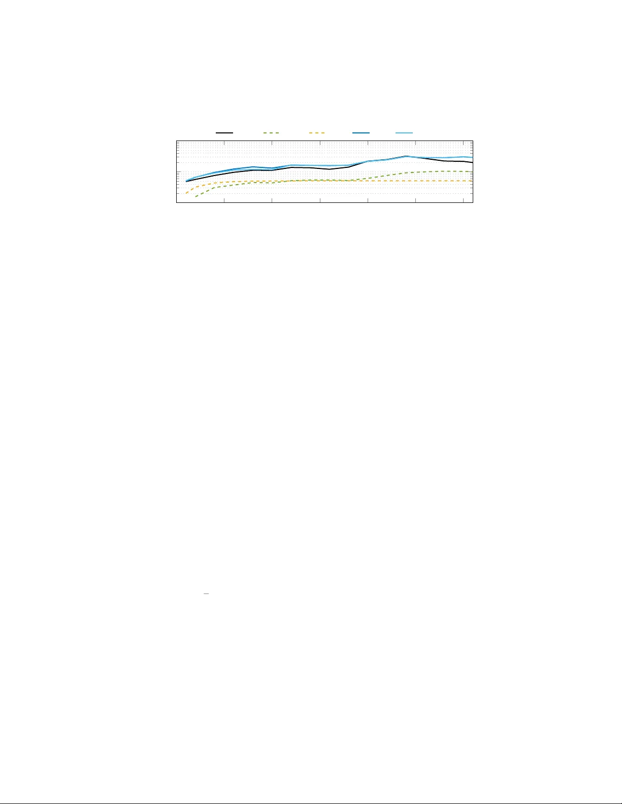
Kernel-based Inference of F unctions o v er Graphs V assilis N. Ioannidis ? , Meng Ma ? , A thanasios N. Nikolak opoulos ? , Georgios B. Giannakis ? , and Daniel Romero † ∗ April 12, 2018 T o be published as a chapter in ‘ Adaptiv e Learning Methods for Nonlinear System Mo deling ’, Elsevier Publishing, Eds. D. Comminiello and J.C. Principe (2018) Abstract The study of net works has witnessed an explosive gro wth ov er the past decades with sev eral ground-breaking methods in tro duced. A par- ticularly interesting – and prev alent in several fields of study – problem is that of inferring a function define d over the nodes of a network . This w ork presents a versatile kernel-based framework for tac kling this infer- ence problem that naturally subsumes and generalizes the reconstruction approac hes put forth recently by the signal processing on graphs commu- nit y . Both the static and the dynamic settings are considered along with effectiv e modeling approac hes for addressing real-w orld problems. The herein analytical discussion is complemented by a set of numerical exam- ples, which sho wcase the effectiveness of the presented techniques, as well as their merits related to state-of-the-art metho ds. Index terms— Signal Processing on Graphs, Kernel-based learning, Graph function reconstruction, Dynamic graphs, Kernel Kalman filter 1 In tro duction Numerous applications arising in div erse disciplines inv olve infer enc e over net- works [1]. Mo delling nodal attributes as signals that tak e v alues ov er the vertices of the underlying graph, allo ws the asso ciated inference tasks to leverage no de dep endencies captured by the graph structure. In many real settings one often affords to work with only a limited num b er of no de observ ations due to inher- en t restrictions particular to the inference task at hand. In so cial netw orks, for example, individuals ma y b e reluctant to share p ersonal information; in sensor net works the nodes may rep ort observ ations sp oradically in order to sav e energy; ∗ ? ECE Dept. and the Digital T ech. Cen ter, Univ. of Minnesota, Mpls, MN 55455, USA. E-mails: { ioann006,maxxx971,anikolak,georgios } @umn.edu, and † Dept. of In- formation and Communication T echnology Universit y of Agder, Grimstad, Norwa y E-mail: daniel.romero@uia.no 1 in brain net works acquiring no de samples ma y inv olve inv asive pro cedures (e.g. electro corticograph y). In this con text, a frequently encountered challenge that often emerges is that of inferring the attributes for every no de in the network given the attributes for a subset of no des . This is typically form ulated as the task of reconstructing a function defined on the no des [1 – 6], given information ab out some of its v alues. Reconstruction of functions o ver graphs has been studied b y the machine learning comm unity , in the context of semi-sup ervise d le arning under the term of tr ansductive regression and classification [6 – 8]. Existing approaches assume “smo othness” with resp ect to the graph – in the sense that neighboring v ertices ha ve similar v alues – and devise nonp ar ametric metho ds [2, 3, 6, 9] targeting pri- marily the task of reconstructing binary-v alued signals. F unction estimation has also b een inv estigated recently b y the communit y of signal pro cessing on graphs (SP oG) under the term signal r e c onstruction [10 – 17]. Most suc h approaches commonly adopt p ar ametric estimation to ols, and rely on b and limite dness , by whic h the signal of interest is assumed to lie in the span of the B principal eigen vectors of the graph’s Laplacian (or adjacency) matrix. This chapter cross-pollinates ideas arising from b oth communities, and presen ts a unifying framework for tackling signal reconstruction problems both in the traditional time-invariant , as well as in the more challenging time-varying set- ting. W e begin by a comprehensiv e presentation of k ernel-based learning for solving problems of signal reconstruction ov er graphs (Section 2). Data-driven tec hniques are then presented based on multi-k ernel learning (MKL) that en- ables combining optimally the k ernels in a given dictionary , and sim ultaneously estimating the graph function by solving a single optimization problem (Sec- tion 2.3). F or the case where prior information is av ailable, semi-parametric estimators are discussed that can incorp orate seamlessly structured prior infor- mation into the signal estimators (Section 2.4). W e then mo ve to the problem of reconstructing time-evolving functions on dynamic graphs (Section 3). The k ernel-based framework is no w extended to accommo date the time-evolving set- ting building on the notion of gr aph extension , sp ecific choices of whic h can lend themselv es to a reduced complexity online solver (Section 3.1). Next, a more flexible mo del is in tro duced that captures multiple forms of time dynamics, and k ernel-based learning is employ ed to derive an online solver, that effects online MKL by selecting the optimal combination of kernels on-the-fly (Section 3.2). Our analytical exp osition, in b oth parts, is supplemented by a set of numeri- cal tests based on b oth real and synthetic data that highlight the effectiveness of the metho ds, while providing examples of interesting realistic problems that they can address. Notation : Scalars are denoted b y low ercase characters, vectors by b old lo w- ercase, matrices by b old upp ercase; ( A ) m,n is the ( m, n )-th entry of matrix A ; sup erscripts T and † resp ectiv ely denote transp ose and pseudo-inv erse. If A := [ a 1 , . . . , a N ], then vec { A } := [ a T 1 , . . . , a T N ] T := a . With N × N matrices { A t } T t =1 and { B t } T t =2 satisfying A t = A T t ∀ t , btridiag { A 1 , . . . , A T ; B 2 , . . . , B T } represen ts the symmetric blo ck tridiagonal matrix. Sym b ols  , ⊗ , and ⊕ re- sp ectiv ely denote element-wise (Hadamard) matrix product, Kronec ker pro duct, 2 and Kronec ker sum, the latter b eing defined for A ∈ R M × M and B ∈ R N × N as A ⊕ B := A ⊗ I N + I M ⊗ B . The n -th column of the iden tity matrix I N is represen ted b y i N ,n . If A ∈ R N × N is positive definite and x ∈ R N , then || x || 2 A := x T A − 1 x and || x || 2 := || x || I N . The cone of N × N positive definite matrices is denoted by S N + . Finally , δ [ · ] stands for the Kroneck er delta, and E for exp ectation. 2 Reconstruction of F unctions o v er Graphs Before giving the formal problem statement, it is instructive to start with the basic definitions that will b e used throughout this c hapter. Definitions : A graph can b e sp ecified by a tuple G := ( V , A ), where V := { v 1 , . . . , v N } is the vertex set, and A is the N × N adjacency matrix, whose ( n, n 0 )-th en try , A n,n 0 ≥ 0, denotes the non-negative edge weigh t b et ween ver- tices v n and v n 0 . F or simplicity , it is assumed that the graph has no self-lo ops, i.e. A n,n = 0 , ∀ v n ∈ V . This chapter fo cuses on undir e cte d graphs, for which A n 0 ,n = A n,n 0 ∀ v n , v n 0 ∈ V . A graph is said to b e unweighte d if A n,n 0 is either 0 or 1. The edge set is defined as E := { ( v n , v n 0 ) ∈ V × V : A n,n 0 6 = 0 } . Tw o v ertices v n and v n 0 are adjac ent , c onne cte d , or neighb ors if ( v n , v n 0 ) ∈ E . The L aplacian matrix is defined as L := diag { A1 } − A , and is symmetric and p os- itiv e semidefinite [1, Ch. 2]. A real-v alued function (or signal) on a graph is a map f : V → R . The v alue f ( v ) represen ts an attribute or feature of v ∈ V , such as age, political alignment, or annual income of a p erson in a so cial net work. Signal f is thus represented by f := [ f ( v 1 ) , . . . , f ( v N )] T . Problem statement. Supp ose that a collection of noisy samples (or obser- v ations) { y s | y s = f ( v n s ) + e s } S s =1 is av ailable, where e s mo dels noise and S := { n 1 , . . . , n S } con tains the indices 1 ≤ n 1 < · · · < n S ≤ N of the sam- pled vertices, with S ≤ N . Given { ( n s , y s ) } S s =1 , and assuming knowledge of G , the goal is to estimate f . This will provide estimates of f ( v ) b oth at observed and unobserved vertices.By defining y := [ y 1 , . . . , y S ] T , the observ ation mo del is summarized as y = Sf + e (1) where e := [ e 1 , . . . , e S ] T and S is a known S × N binary sampling matrix with en tries ( s, n s ), s = 1 , . . . , S , set to one, and the rest set to zero. 2.1 Kernel Regression Kernel metho ds constitute the “workhorse” of machine learning for nonlinear function estimation [18]. Their p opularity can be attributed to their simplic- it y , flexibilit y , and goo d p erformance. Here, w e present k ernel regression as a unifying framework for graph signal reconstruction along with the so-called represen ter theorem. Kernel regression seeks an estimate of f in a repro ducing kernel Hilb ert space 3 (RKHS) H , which is the space of functions f : V → R defined as H := ( f : f ( v ) = N X n =1 α n κ ( v , v n ) , α n ∈ R ) (2) where the kernel map κ : V × V → R is any function defining a symmetric and p ositive semidefinite N × N matrix with en tries [ K ] n,n 0 := κ ( v n , v n 0 ) [19]. In tuitively , κ ( v , v 0 ) is a basis function in (2) measuring similarit y b etw een the v alues of f at v and v 0 . (F or a more detailed treatment of RKHS, see e.g. [3]). Note that for signals o ver graphs, the expansion in (2) is finite since V is finite-dimensional. Th us, any f ∈ H can b e expressed in compact form f = K α (3) for some N × 1 vector α := [ α 1 , . . . , α N ] T . Giv en tw o functions f ( v ) := P N n =1 α n κ ( v , v n ) and f 0 ( v ) := P N n =1 α 0 n κ ( v , v n ), their RKHS inner pro duct is defined as 1 h f , f 0 i H := N X n =1 N X n 0 =1 α n α 0 n 0 κ ( v n , v n 0 ) = α T K α 0 (4) where α 0 := [ α 0 1 , . . . , α 0 N ] T and the repro ducing prop erty has been employ ed that suggests h κ ( · , v n 0 ) , κ ( · , v n 0 0 ) i H = i T n 0 Ki n 0 0 = κ ( v n 0 , v n 0 0 ). The RKHS norm is defined by || f || 2 H := h f , f i H = α T K α (5) and will be used as a regularizer to control ov erfitting and to cop e with the under-determined reconstruction problem. As a special case, setting K = I N reco vers the standard inner pro duct h f , f 0 i H = f T f 0 , and the Euclidean norm || f || 2 H = || f || 2 2 . Note that when K  0 , the set of functions of the form (3) coincides with R N . Giv en { y s } S s =1 , RKHS-based function estimators are obtained by solving functional minimization problems formulated as (see also e.g. [18 – 20]) ˆ f := arg min f ∈H L ( y , ¯ f ) + µ Ω( || f || H ) (6) where the loss L measures how the estimated function f at the observ ed v ertices { v n s } S s =1 , collected in ¯ f := [ f ( v n 1 ) , . . . , f ( v n S )] T = Sf , deviates from the data y . The so-called squar e loss L ( y , ¯ f ) := (1 /S ) P S s =1 [ y s − f ( v n s )] 2 constitutes a p opular c hoice for L . The increasing function Ω is used to promote smo othness with t ypical choices including Ω( ζ ) = | ζ | and Ω( ζ ) = ζ 2 . The regularization 1 While f denotes a function , f ( v ) represents the sc alar resulting from ev aluating f at vertex v . 4 parameter µ > 0 controls ov erfitting. Substituting (3) and (5) into (6) shows that ˆ f can b e found as ˆ α := arg min α ∈ R N L ( y , SK α ) + µ Ω(( α T K α ) 1 / 2 ) (7a) ˆ f = K ˆ α . (7b) An alternativ e form of (5) that will be frequen tly used in the sequel results up on noting that α T K α = α T KK † K α = f T K † f . (8) Th us, one can rewrite (6) as ˆ f := arg min f ∈R{ K } L ( y , Sf ) + µ Ω(( f T K † f ) 1 / 2 ) . (9) Although graph signals can b e reconstructed from (7), such an approac h in volv es optimizing ov er N v ariables. Thankfully , the solution can b e obtained b y solving an optimization problem in S v ariables (where typically S  N ), b y in voking the so-called representer theorem [19, 21]. The representer theorem pla ys an instrumental role in the traditional infinite- dimensional setting where (6) cannot b e solved directly; how ever, ev en when H comprises graph signals, it can s till b e b eneficial to reduce the dimension of the optimization in (7). The theorem essentially asserts that the solution to the functional minimization in (6) can b e expressed as ˆ f ( v ) = S X s =1 ¯ α s κ ( v , v n s ) (10) for some ¯ α s ∈ R , s = 1 , . . . , S . The representer theorem shows the form of ˆ f , but do es not provide the optimal { ¯ α s } S s =1 , which are found after substituting (10) in to (6), and solving the resulting optimization problem with respect to these coefficients. T o this end, let ¯ α := [ ¯ α 1 , . . . , ¯ α S ] T , and write α = S T ¯ α to deduce that ˆ f = K α = KS T ¯ α . (11) With ¯ K := SKS T and using (7) and (11), the optimal ¯ α can b e found as ˆ ¯ α := arg min ¯ α ∈ R S L ( y , ¯ K ¯ α ) + µ Ω(( ¯ α T ¯ K ¯ α ) 1 / 2 ) . (12) Kernel ridge regression . F or L chosen as the square loss and Ω( ζ ) = ζ 2 , the ˆ f in (6) is referred to as the kernel ridge r e gr ession (RR) estimate [18]. If ¯ K is full rank, this estimate is given by ˆ f RR = KS T ˆ ¯ α , where ˆ ¯ α := arg min ¯ α ∈ R S 1 S   y − ¯ K ¯ α   2 + µ ¯ α T ¯ K ¯ α (13a) = ( ¯ K + µS I S ) − 1 y . (13b) 5 Therefore, ˆ f RR can b e expressed as ˆ f RR = KS T ( ¯ K + µS I S ) − 1 y . (14) As we will see in the next section, (14) generalizes a num b er of existing signal reconstructors up on prop erly selecting K . 2.2 Kernels on Graphs When estimating functions on graphs, con ven tional k ernels suc h as the Gaussian k ernel cannot b e adopted because the underlying set where graph signals are defined is not a metric space. Indeed, no vertex addition v n + v n 0 , scaling β v n , or norm || v n || can b e naturally defined on V . An alternative is to embed V in to Euclidean space via a feature map φ : V → R D , and inv oke a con v entional kernel afterw ards. Ho wev er, for a given graph it is generally unclear how to explicitly design φ or select D . This motiv ates the adoption of kernels on gr aphs [3]. A common approac h to designing kernels on graphs is to apply a transforma- tion function on the graph Laplacian [3]. The term L aplacian kernel comprises a wide family of kernels obtained by applying a certain function r ( · ) to the Laplacian matrix L . Laplacian kernels are well motiv ated since they constitute the graph coun terpart of the so-called tr anslation-invariant kernels in Euclidean spaces [3]. This section reviews Laplacian k ernels, pro vides b eneficial insights in terms of interpolating signals, and highligh ts their v ersatility in capturing information ab out the gr aph F ourier tr ansform of the estimated signal. The reason why the graph Laplacian constitutes one of the prominent can- didates for regularization on graphs, b ecomes clear up on recognizing that f T Lf = 1 2 X ( n,n 0 ) ∈E A n,n 0 ( f n − f n 0 ) 2 , (15) where A n,n 0 denotes weigh t asso ciated with edge ( n, n 0 ). The quadratic form of (15) b ecomes larger when function v alues v ary a lot among connected v ertices and therefore quantifies the smo othness of f on G . Let 0 = λ 1 ≤ λ 2 ≤ . . . ≤ λ N denote the eigenv alues of the graph Lapla- cian matrix L , and consider the eigendecomp osition L = UΛU T , where Λ := diag { λ 1 , . . . , λ N } . A Laplacian kernel matrix is defined by K := r † ( L ) := U r † ( Λ ) U T (16) where r ( Λ ) is the result of applying a user-selected, scalar, non-negativ e map r : R → R + to the diagonal en tries of Λ . The selection of map r generally dep ends on desirable properties that the target function is expected to ha ve. T able 1 summarizes some well-kno wn examples arising for sp ecific choices of r . A t this p oint, it is pruden t to offer in terpretations and insights on the opera- tion of Laplacian kernels. T o wards this ob jectiv e, note first that the regularizer 6 Kernel name F unction P arameters Diffusion [2] r ( λ ) = exp { σ 2 λ/ 2 } σ 2 p -step random walk [3] r ( λ ) = ( a − λ ) − p a ≥ 2, p ≥ 0 Regularized Laplacian [3, 22] r ( λ ) = 1 + σ 2 λ σ 2 Bandlimited [23] r ( λ ) = ( 1 /β λ ≤ λ max β otherwise β > 0, λ max T able 1: Common sp ectral weigh t functions. from (9) is an increasing function of α T K α = α T KK † K α = f T K † f = f T U r ( Λ ) U T f = ˇ f T r ( Λ ) ˇ f = N X n =1 r ( λ n ) | ˇ f n | 2 (17) where ˇ f := U T f := [ ˇ f 1 , . . . , ˇ f N ] T comprises the pro jections of f on to the eigenspace of L , and is referred to as the gr aph F ourier tr ansform of f in the SP oG parlance [4]. Consequen tly , { ˇ f n } N n =1 are called fr e quency c omp onents . The so-called b and limite d functions in SPoG refer to those whose frequency comp onen ts only exist inside some band B , that is, ˇ f n = 0 , ∀ n > B . By adopting the aforementioned SPoG notions, one can intuitiv ely interpret the role of bandlimited kernels. Indeed, it follows from (17) that the regularizer strongly p enalizes those ˇ f n for which the corresp onding r ( λ n ) is large, thus promoting a sp ecific structure in this “frequency” domain. Sp ecifically , one prefers r ( λ n ) to b e large whenev er | ˇ f n | 2 is small and vice v ersa. The fact that | ˇ f n | 2 is exp ected to decrease with n for smo oth f , motiv ates the adoption of an increasing function r [3]. F rom (17) it is clear that r ( λ n ) determines ho w hea vily ˇ f n is p enalized. Therefore, by setting r ( λ n ) to b e small when n ≤ B and extremely large when n > B , one can exp ect the result to b e a bandlimited signal. Observ e that Laplacian k ernels can capture forms of prior information ric her than bandlimitedness [11, 13, 16, 17] by selecting function r accordingly . F or instance, using r ( λ ) = exp { σ 2 λ/ 2 } (diffusion k ernel) accounts not only for smo othness of f as in (15), but also for the prior that f is generated by a pro cess diffusing ov er the graph. Similarly , the use of r ( λ ) = ( α − λ ) − 1 (1-step random walk) can accommodate cases where the signal captures a notion of net work centralit y 2 . So far, f has b een assumed deterministic, whic h precludes accommo dating certain forms of prior information that probabilistic mo dels can capture, such 2 Smola et al. [3], for example, discuss the connection b etw een r ( λ ) = ( α − λ ) − 1 and PageRank [24] whereb y the sought-after signal is essentially defined as the limiting distribution of a simple underlying “ r andom surfing ” process. F or more ab out random surfing pro cesses, see also [25, 26]. 7 as domain kno wledge and historical data. Suppose without loss of generalit y that { f ( v n ) } N n =1 are zero-mean random v ariables. The LMMSE estimator of f given y in (1) is the linear estimator ˆ f LMMSE minimizing E || f − ˆ f LMMSE || 2 2 , where the exp ectation is o ver all f and noise realizations. With C := E  f f T  , the LMMSE estimate is ˆ f LMMSE = CS T [ SCS T + σ 2 e I S ] − 1 y (18) where σ 2 e := (1 /S ) E  || e || 2 2  denotes the noise v ariance. Comparing (18) with (14) and recalling that ¯ K := SKS T , it follows that ˆ f LMMSE = ˆ f RR if µS = σ 2 e and K = C . In other words, the similarity measure κ ( v n , v n 0 ) embo died in such a k ernel map is just the co v ariance cov[ f ( v n ) , f ( v n 0 )]. A related observ ation was p oin ted out in [27] for general kernel methods. In short, one can interpret kernel ridge regression as the LMMSE estimator of a signal f with co v ariance matrix equal to K ; see also [28]. The LMMSE in terpretation also suggests the usage of C as a k ernel matrix, which enables signal reconstruction ev en when the graph top ology is unknown. Although this discussion hinges on kernel ridge regression after setting K = C , any other k ernel estimator of the form (7) can b enefit from vertex-co v ariance kernels to o. In most contemporary net works, sets of nodes ma y depend among eac h other via m ultiple t yp es of relationships, which ordinary net works cannot capture [29]. Consequen tly , generalizing the traditional single-layer to multilayer netw orks that organize the nodes in to different groups, called layers ,is w ell motiv ated. F or kernel-based approaches for function reconstruction ov er multila yer graphs see also [30]. 2.3 Selecting k ernels from a dictionary The selection of the p ertinent kernel matrix is of paramount imp ortance to the p erformance of kernel-based metho ds [23, 31]. This section presents an MKL approach that effects kernel selection in graph signal reconstruction. Tw o algorithms with complementary strengths will b e presented. Both rely on a user-sp ecified kernel dictionary , and the b est kernel is built from the dictionary in a data driven w ay . The first algorithm, which w e call RKHS sup erp osition , is motiv ated b y the fact that one sp ecific H in (6) is determined by some κ ; therefore, kernel selection is tantamoun t to RKHS selection. Consequently , a kernel dictionary { κ m } M m =1 giv es rise to a RKHS dictionary {H m } M m =1 , whic h motiv ates estimates of the form 3 ˆ f = M X m =1 ˆ f m , ˆ f m ∈ H m . (19) Up on adopting a criterion that con trols sparsity in this expansion, the “b est” RKHSs will be selected. A reasonable approac h is therefore to generalize (6) 3 A sum is chosen here for tractability , but the right-hand side of (19) could in principle combine the functions { ˆ f m } m in different forms. 8 to accommo date m ultiple RKHSs. With L selected to b e the square loss and Ω( ζ ) = | ζ | , one can pursue an estimate ˆ f b y solving min { f m ∈H m } M m =1 1 S S X s =1 " y s − M X m =1 f m ( v n s ) # 2 + µ M X m =1 k f m k H m . (20) In voking the representer theorem p er f m establishes that the minimizers of (20) can b e written as ˆ f m ( v ) = S X s =1 ¯ α m s κ m ( v , v n s ) , m = 1 , . . . , M (21) for some co efficien ts ¯ α m s . Substituting (21) into (20) suggests obtaining these co efficien ts as arg min { ¯ α m } M m =1 1 S      y − M X m =1 ¯ K m ¯ α m      2 + µ M X m =1  ¯ α T m ¯ K m ¯ α m  1 / 2 (22) where ¯ α m := [ ¯ α m 1 , . . . , ¯ α m S ] T , and ¯ K m := SK m S T with ( K m ) n,n 0 := κ m ( v n , v n 0 ). Letting ˇ ¯ α m := ¯ K 1 / 2 m ¯ α m , expression (22) b ecomes arg min { ˇ ¯ α m } M m =1 1 S      y − M X m =1 ¯ K 1 / 2 m ˇ ¯ α m      2 + µ M X m =1 k ˇ ¯ α m k 2 . (23) In terestingly , (23) can b e efficiently solv ed using the alternating-direction metho d of m ultipliers (ADMM) [32, 33] after some nessecary reformulation [23]. After obtaining { ˇ ¯ α m } M m =1 , the sought-after function estimate can b e recov- ered as ˆ f = M X m =1 K m S T ¯ α m = M X m =1 K m S T ¯ K − 1 / 2 m ˇ ¯ α m . (24) This MKL algorithm can iden tify the b est subset of RKHSs – and therefore k ernels – but entails M S unkno wns (cf. (22)). Next, an alternative approach is discussed which can reduce the num b er of v ariables to M + S at the price of not b eeing able to assure a sparse kernel expansion. The alternative approach is to p ostulate a kernel of the form K ( θ ) = P M m =1 θ m K m , where { K m } M m =1 is given and θ m ≥ 0 ∀ m . The co efficients θ := [ θ 1 , . . . , θ M ] T can b e found by jointly minimizing (12) with resp ect to θ and ¯ α [34] ( θ , ˆ ¯ α ) := arg min θ , ¯ α 1 S L ( v , y , ¯ K ( θ ) ¯ α ) + µ Ω(( ¯ α T ¯ K ( θ ) ¯ α ) 1 / 2 ) (25) where ¯ K ( θ ) := SK ( θ ) S T . Except for degenerate cases, problem (25) is not join tly conv ex in θ and ˆ ¯ α , but it is separately con vex in each v ector for a conv ex L [34]. Iterative algorithms for solving (23) and (25) are av ailable in [23]. 9 2.4 Semi-parametric reconstruction The approac hes discussed so far are applicable to v arious problems but they are certainly limited by the mo deling assumptions they make. In particular, the p erformance of algorithms b elonging to the parametric family [11, 15, 35] is restricted by how well the signals actually adhere to the selected mo del. Non- parametric mo dels on the other hand [2, 3, 6, 36], offer flexibilit y and robustness but they cannot readily incorp orate information av ailable a priori. In practice ho wev er, it is not uncomm on that neither of these approac hes alone suffices for reliable inference. Consider, for instance, an employmen t- orien ted so cial netw ork such as LinkedIn, and supp ose the goal is to estimate the salaries of all users given information about the salaries of a few. Clearly , be- sides net work connections, exploiting av ailable information regarding the users’ education level and work exp erience could b enefit the reconstruction task. The same is true in problems arising in link analysis, where the exploitation of W eb’s hierarc hical structure can aid the task of estimating the imp ortance of W eb pages [37]. In recommender systems, inferring preference scores for ev ery item, giv en the users’ feedbac k ab out particular items, could be cast as a signal recon- struction problem o v er the item correlation graph. Data sparsity imp oses sev ere limitations in the qualit y of pure collab orative filtering metho ds [38] Exploiting side information ab out the items, is kno wn to alleviate suc h limitations [39], leading to considerably improv ed recommendation p erformance [40, 41]. A promising direction to endow nonparametric metho ds with prior informa- tion relies on a semi-p ar ametric approac h whereby the signal of interest is mo d- eled as the sup erp osition of a parametric and a nonparametric comp onent [42]. While the former leverages side information, the latter accounts for deviations from the parametric part, and can also promote smo othness using kernels on graphs. In this section w e outline tw o simple and reliable semi-parametric esti- mators with complementary strengths, as detailed in [42]. 2.4.1 Semi-parametric Inference F unction f is mo deled as the sup erp osition 4 f = f P + f NP (26) where f P := [ f P ( v 1 ) , . . . , f P ( v N )] T , and f NP := [ f NP ( v 1 ) , . . . , f NP ( v N )] T . The parametric term f P ( v ) := P M m =1 β m b m ( v ) captures the known signal structure via the basis B := { b m } M m =1 , while the nonparametric term f NP b e- longs to an RKHS H , which accounts for deviations from the span of B . The goal of this section is efficient and reliable estimation of f giv en y , S , B , H and G . Since f NP ∈ H , v ector f NP can b e represen ted as in (3). By defining β := [ β 1 , . . . , β M ] T , and the N × M matrix B with entries ( B ) n,m := b m ( v n ), 4 for simplicity here we consider only the case of semi-parametric partially linear models. 10 the parametric term can be written in v ector form as f P := B β . The semi- parametric estimates can b e found as the solution of the follo wing optimization problem { ˆ α , ˆ β } = arg min α , β 1 S S X s =1 L ( y s , f ( v n s )) + µ k f NP k 2 H (27) s.t. f = B β + K α where the fitting loss L quantifies the deviation of f from the data, and µ > 0 is the regularization scalar that controls o verfitting the nonparametric term. Using (27), the semi-parametric e stimates are expressed as ˆ f = B ˆ β + K ˆ α . Solving (27) entails minimization ov er N + M v ariables. Clearly , when deal- ing with large-scale graphs this could lead to prohibitively large computational cost. T o reduce complexity , the semi-parametric version of the representer the- orem [18, 19] is employ ed, which establishes that ˆ f = B ˆ β + KS T ˆ ¯ α (28) where ˆ ¯ α := [ ˆ ¯ α 1 , . . . , ˆ ¯ α S ] T . Estimates ˆ ¯ α , ˆ β are found as { ˆ ¯ α , ˆ β } = arg min ¯ α , β 1 S S X s =1 L ( y s , f ( v n s )) + µ k f NP k 2 H (29) s.t. f = B β + KS T ¯ α where ¯ α := [ ¯ α 1 , . . . , ¯ α S ] T . The RKHS norm in (29) is expressed as k f NP k 2 H = ¯ α T ¯ K ¯ α , with ¯ K := SKS T . Relative to (27), the num b er of optimization v ari- ables in (29) is reduced to the more affordable S + M , with S  N . Next, t wo loss functions with complementary b enefits will b e considered: the squar e loss and the  -insensitive loss. The square loss function is L ( y s , f ( v n s )) := k y s − f ( v n s )) k 2 2 (30) and (29) admits the following closed-form solution ˆ ¯ α = ( P ¯ K + µ I S ) − 1 Py (31a) ˆ β = ( ¯ B T ¯ B ) − 1 ¯ B T ( y − ¯ K ˆ ¯ α ) (31b) where ¯ B := SB , P := I S − ¯ B ( ¯ B T ¯ B ) − 1 ¯ B T . The complexity of (31) is O ( S 3 + M 3 ). The  -insensitive loss function is given by L ( y s , f ( v n s )) := max(0 , | y s − f ( v n s ) | −  ) (32) where  is tuned, e.g. via cross-v alidation, to minimize the generalization error and has well-documented merits in signal estimation from quantized data [43]. Substituting (32) into (29) yields a conv ex non-smo oth quadratic problem that can b e solved efficiently for ¯ α and β using e.g. in terior-p oint metho ds [18]. 11 2.5 Numerical tests This section rep orts on the signal reconstruction p erformance of differen t meth- o ds using real as well as synthetic data. The p erformance of the estimators is assessed via Monte Carlo simulation by comparing the normalized mean-square error (NMSE) NMSE = E  k ˆ f − f k 2 k f k 2  . (33) Multi-k ernel reconstruction. The first data set contains departure and ar- riv al information for flights among U.S. airp orts [44], from which 3 × 10 6 fligh ts in the months of July , August, and Septem b er of 2014 and 2015 were selected. W e construct a graph with N = 50 vertices corresp onding to the airp orts with highest traffic, and whenever the num b er of fligh ts b etw een the t wo airp orts ex- ceeds 100 within the observ ation window, we connect the corresp onding no des with an edge. A signal was constructed p er day av eraging the arriv al delay of al l inbound fligh ts p er selected airp ort. A total of 184 signals were considered, of whic h the first 154 were used for training (July , August, Septem b er 2014, and July , August 2015), and the remaining 30 for testing (September 2015). The w eights of the edges betw een airp orts were learned using the training data based on the tec hnique describ ed in [23]. Multi-Kernel Reconstruction NMSE RMSE[min] KRR with cov. Kernel 0.34 3.95 Multi-k ernel, RS 0.44 4.51 Multi-k ernel, KS 0.43 4.45 BL for B=2 1.55 8.45 BL for B=3 32.64 38.72 BL, cut-off 3.97 13.5 T able 2: Multi-Kernel Reconstruction T able 2 lists the NMSE and the RMSE in minutes for the task of predicting the arriv al dela y at 40 airp orts when the delay at a randomly selected collection of 10 airp orts is observed. The second row corresp onds to the ridge regression estimator that uses the nearly-optimal estimate d cov ariance kernel. The next t wo ro ws correspond to the multi-k ernel approaches in § 2.3 with a dictionary of 30 diffusion kernels with v alues of σ 2 uniformly spaced b etw een 0.1 and 7. The rest of the rows p ertain to graph-bandlimited estimators (BL). T able 2 demonstrates the reliable performance of co v ariance kernels as w ell as the herein discussed multi-k ernel approac hes relative to comp eting alternatives. 12 NMSE of the synthetic signal estimates. 50 100 150 200 10 − 0 . 5 10 0 10 0 . 5 Number of observed nodes (S) NMSE SP-GK SP-GK(  ) (a) ( µ = 5 × 10 − 4 , σ = 5 × 10 − 4 , SNR e = 5dB). 50 100 150 200 10 − 1 10 0 Number of observed nodes (S) NMSE BL B = 10 BL B = 20 P NP SP-GK (b) ( µ = 5 × 10 − 4 , σ = 5 × 10 − 4 ,  = 10 − 4 , and SNR o = − 5dB). Figure 1: NMSE of the synthetic signal estimates. 13 Semi-parametric reconstruction. An Erd˝ os-R ` en yi graph with probabilit y of edge presence 0 . 6 and N = 200 no des was generated, and f was formed by sup erimp osing a bandlimited signal [13, 15] plus a piecewise constant signal [45]; that is, f = 10 X i =1 γ i u i + 6 X i =1 δ i 1 V c (34) where { γ i } 10 i =1 and { δ i } 6 i =1 are standardized Gaussian distributed; { u i } 10 i =1 are the eigenv ectors associated with the 10 smallest eigen v alues of the Laplacian ma- trix; {V i } 6 i =1 are the v ertex sets of 6 clusters obtained via spectral clustering [46]; and 1 V i is the indicator vector with entries ( 1 V i ) n := 1, if v n ∈ V i , and 0 other- wise. The parametric basis B = { 1 V i } 6 i =1 w as used by the estimators capturing the prior knowledge, and S vertices were sampled uniformly at random. The subsequen t exp erimen ts ev aluate the p erformance of the semi-parametric graph k ernel estimators, SP-GK and SP-GK(  ) resulting from using (30) and (32) in (29), resp ectively; the p ar ametric (P) that considers only the parametric term in (26); the nonp ar ametric (NP) [2, 3] that considers only the nonpara- metric term in (26); and the graph-bandlimited estimators (BL) from [13, 15], whic h assume a bandlimited mo del with bandwidth B . F or all the experiments, the diffusion kernel (cf. T able 1) with parameter σ is employ ed. First, white Gaussian noise e s of v ariance σ 2 e is added to eac h sample f s to yield signal- to-noise ratio SNR e := k f k 2 2 / ( N σ 2 e ). Fig. 1(b) presents the NMSE of differen t metho ds. As exp ected, the limited flexibility of the parametric approaches, B L and P , affects their ability to capture the true signal structure. The NP esti- mator ac hieves smaller NMSE, but only when the amount of av ailable samples is adequate. Both semi-parametric estimators were found to outp erform other approac hes, exhibiting reliable reconstruction even with few samples. T o illustrate the b enefits of employing different loss functions (30) and (32), w e compare the p erformance of SP-GK and SP-GK(  ) in the presence of outlying noise. Eac h sample f s is contaminated with Gaussian noise o s of large v ariance σ 2 o with probability p = 0 . 1. Fig. 1(a) demonstrates the robustness of SP-GK(  ) whic h is attributed to the  − insensitive loss function (32). F urther exp eriments using real signals can b e found in [42]. 3 Inference of dynamic functions o v er dynamic graphs Net works that exhibit time-varying c onne ctivity patterns with time-varying no de attributes arise in a plethora of net work science related applications. Sometimes these dynamic netw ork topologies switch b etw een a finite num b er of discrete states, gov erned by sudden changes of the underlying dynamics [47, 48]. A c hal- lenging problem that arises in this setting is that of reconstructing time-ev olving functions on graphs, given their v alues on a subset of vertices and time instants. Efficien tly exploiting spatiotemp oral dynamics can markedly impact sampling 14 costs by reducing the num b er of v ertices that need to b e observed to attain a target p erformance. Such a reduction can b e of paramount imp ortance in cer- tain applications eg. in monitoring time-dep endent activity of different regions of the brain through inv asive electro corticography (ECoG), where observing a v ertex requires the implantation of an in tracranial electro de [47]. Although one could reconstruct a time-v arying function per time slot us- ing the non- or semi-parametric metho ds of § 2, lev eraging time correlations t ypically yields estimators with improv ed p erformance. Schemes tailored for time-ev olving functions on graphs include [49] and [50], whic h predict the func- tion v alues at time t given observ ations up to time t − 1. Ho wev er, these sc hemes assume that the function of interest adheres to a sp ecific vector autoregressive mo del. Other works target time-inv arian t functions, but can only afford track- ing sufficien tly slo w v ariations. This is the case with the dictionary learning approac h in [51] and the distributed algorithms in [52] and [53]. Unfortunately , the flexibility of these algorithms to capture spatial information is also limited since [51] fo cuses on Laplacian regularization, whereas [52] and [53] require the signal to b e bandlimited. Motiv ated by the aforementioned limitations, in what comes next we extend the framework presen ted in § 2 accommo dating time-v arying function reconstruc- tion ov er dynamic graphs. But b efore we delv e into the time-v arying setting, a few definitions are in order. Definitions : A time-v arying graph is a tuple G ( t ) := ( V , A t ), where V := { v 1 , . . . , v N } is the v ertex set, and A t ∈ R N × N is the adjacency matrix at time t , whose ( n, n 0 )-th en try A n,n 0 ( t ) assigns a w eigh t to the pair of v ertices ( v n , v n 0 ) at time t . A time-in v ariant graph is a special case with A t = A t 0 ∀ t, t 0 . Adopting common assumptions made in related literature (e.g. [1, Ch. 2], [4, 9]), we also define G ( t ) (i) to hav e non-negative weigh ts ( A n,n 0 ( t ) ≥ 0 ∀ t, and ∀ n 6 = n 0 ); (ii) to hav e no self-edges ( A n,n ( t ) = 0 ∀ n, t ); and, (iii) to b e undirected ( A n,n 0 ( t ) = A n 0 ,n ( t ) ∀ n, n 0 , t ). A time-v arying function or signal on a graph is a map f : V × T → R , where T := { 1 , 2 , . . . } is the set of time indices. The v alue f ( v n , t ) of f at vertex v n and time t , can b e thought of as the v alue of an attribute of v n ∈ V at time t . The v alues of f at time t will b e collected in f t := [ f ( v 1 , t ) , . . . , f ( v N , t )] T . A t time t , vertices with indices in the time-dep endent set S t := { n 1 ( t ) , . . . , n S ( t ) ( t ) } , 1 ≤ n 1 ( t ) < · · · < n S ( t ) ( t ) ≤ N , are observed. The resulting samples can b e expressed as y s ( t ) = f ( v n s ( t ) , t ) + e s ( t ) , s = 1 , . . . , S ( t ), where e s ( t ) mo dels ob- serv ation error. By letting y t := [ y 1 ( t ) , . . . , y S ( t ) ( t )] T , the observ ations can b e con venien tly expressed as y t = S t f t + e t , t = 1 , 2 , . . . (35) where e t := [ e 1 ( t ) , . . . , e S ( t ) ( t )] T , and the S ( t ) × N sampling matrix S t con tains ones at p ositions ( s, n s ( t )), s = 1 , . . . , S ( t ) and zeros elsewhere. The broad goal of this section is to “reconstruct” f from the observ ations { y t } t in (35). Two formulations will b e considered. Batc h formulation. In the batc h reconstruction problem, one aims at find- ing { f t } T t =1 giv en {G ( t ) } T t =1 , the sample lo cations { S t } T t =1 , and all observ ations 15 { y t } T t =1 . Online formulation. A t every time t , one is given G together with S t and y t , and the goal is to find f t . The latter can b e obtained p ossibly based on a previous estimate of f t − 1 , but the complexity per time slot t must b e indep endent of t . T o solve these problems, we will rely on the assumption that f ev olves smo othly ov er space and time, yet more structured dynamics can b e incor- p orated if known. 3.1 Kernels on extended graphs This section extends the kernel-based learning framew ork of § 2 to subsume time- ev olving functions o v er p ossibly dynamic graphs through the notion of gr aph extension , b y which the time dimension receives the same treatment as the spatial dimension. The versatilit y of kernel-based metho ds to lev erage spatial information [23] is thereby inherited and broadened to account for temp oral dynamics as w ell. This v antage p oin t also accommodates time-v arying sampling sets and top ologies. 3.1.1 Extended graphs An immediate approac h to reconstructing time-ev olving functions is to apply (9) separately for eac h t = 1 , . . . , T . This yields the instan taneous estimator (IE) ˆ f ( I E ) t := arg min f 1 S ( t ) || y t − S t f || 2 2 + µ f T K † t f . (36) Unfortunately , this estimator do es not account for the p ossible relation b etw een e.g. f ( v n , t ) and f ( v n , t − 1). If, for instance, f v aries slowly o ver time, an estimate of f ( v n , t ) ma y as w ell benefit from lev eraging observ ations y s ( τ ) at time instants τ 6 = t . Exploiting temp oral dynamics p otentially reduces the n umber of vertices that ha ve to be sampled to attain a target reconstruction p erformance, which in turn can markedly reduce sampling costs. Incorp orating temp oral dynamics into kernel-based reconstruction, whic h can only handle a single snapshot (cf. § 2), necessitates an appropriate reformu- lation of time-ev olving function reconstruction as a problem of reconstructing a time-inv ariant function. An app ealing p ossibility is to replace G with its ex- tende d version ˜ G := ( ˜ V , ˜ A ), where each v ertex in V is replicated T times to yield the extended v ertex set ˜ V := { v n ( t ) , n = 1 , . . . , N , t = 1 , . . . , T } , and the ( n + N ( t − 1) , n 0 + N ( t 0 − 1))-th entry of the T N × T N extended adjacency matrix ˜ A equals the weigh t of the edge ( v n ( t ) , v n 0 ( t 0 )). The time-v arying function f can th us b e replaced with its extended time-inv ariant counterpart ˜ f : ˜ V → R with ˜ f ( v n ( t )) = f ( v n , t ). Definition 1. L et V := { v 1 , . . . , v N } denote a vertex set and let G := ( V , { A t } T t =1 ) b e a time-varying gr aph. A gr aph ˜ G with vertex set ˜ V := { v n ( t ) , n = 1 , . . . , N , t = 1 , . . . , T } and N T × N T adjac ency matrix ˜ A is an extende d gr aph of G if the t -th N × N diagonal blo ck of ˜ A e quals A t . 16 Figure 2: (a)Original graph (b) Extended graph ˜ G for diagonal B ( T ) t . Edges connecting vertices at the same time instan t are represented by solid lines whereas edges connecting vertices at differen t time instants are represented by dashed lines. In general, the diagonal blo cks { A t } T t =1 do not pro vide full description of the underlying extended graph. Indeed, one also needs to sp ecify the off-diagonal blo c k entries of ˜ A to capture the spatio-temp oral dynamics of f . As an example, consider an extended graph with ˜ A = btridiag { A 1 , . . . , A T ; B ( T ) 2 , . . . , B ( T ) T } (37) where B ( T ) t ∈ R N × N + connects { v n ( t − 1) } N n =1 to { v n ( t ) } N n =1 , t = 2 , . . . , T and btridiag { A 1 , . . . , A T ; B 2 , . . . , B T } represents the symmetric block tridiagonal matrix: ˜ A =          A 1 B T 2 0 . . . 0 0 B 2 A 2 B T 3 . . . 0 0 0 B 3 A 3 . . . 0 0 . . . . . . . . . . . . . . . . . . 0 0 0 . . . A T − 1 B T T 0 0 0 . . . B T A T          . F or instance, each vertex can b e connected to its neighbors at the previous time instant by setting B ( T ) t = A t − 1 , or it can b e connected to its replicas at adjacen t time instants b y setting B ( T ) t to b e diagonal. 3.1.2 Batc h and online reconstruction via space-time kernels The extended graph enables a generalization of the estimators in § 2 for time- ev olving functions. The rest of this subsection discusses tw o such KRR estima- tors. Consider first the batch formulation, where all the ˜ S := P T t =1 S t samples in ˜ y := [ y T 1 , . . . , y T T ] T are av ailable, and the goal is to estimate ˜ f := [ f T 1 , . . . , f T T ] T . Directly applying the KRR criterion in (9) to reconstruct ˜ f on the extended graph ˜ G yields ˆ ˜ f := arg min ˜ f || ˜ y − ˜ S ˜ f || 2 D + µ ˜ f T ˜ K † ˜ f (38a) 17 where ˜ K is now a T N × T N “space-time” kernel matrix, ˜ S := b diag { S 1 , . . . , S T } , and D := b diag  S (1) I S (1) , . . . , S ( T ) I S ( T )  . If ˜ K is inv ertible, (38a) can b e solved in closed form as ˆ ˜ f = ˜ K ˜ S T ( ˜ S ˜ K ˜ S T + µ D ) − 1 ˜ y . (38b) The “space-time” kernel ˜ K , captures complex spatiotemp oral dynamics. If the top ology is time in v ariant, ˜ K can b e specified in a bidimensional plane of spatio- temp oral frequency similar to § 2.2 5 . In the online formulation, one aims to estimate f t after the ˜ S ( t ) := P t τ =1 S ( τ ) samples in ˜ y t := [ y T 1 , . . . , y T t ] T b ecome av ailable. Based on these samples, the KRR estimate of ˜ f , denoted as ˆ ˜ f 1: T | t , is clearly ˆ ˜ f 1: T | t := arg min ˜ f || ˜ y t − ˜ S t ˜ f || 2 D t + µ ˜ f T ˜ K − 1 ˜ f (39a) = ˜ K ˜ S T t ( ˜ S t ˜ K ˜ S T t + µ D t ) − 1 ˜ y t . (39b) where ˜ K is assumed inv ertible for simplicity , D t := b diag  S (1) I S (1) , . . . , S ( t ) I S ( t )  , and ˜ S t := [diag { S 1 , . . . , S t } , 0 ˜ S ( t ) × ( T − t ) N ] ∈ { 0 , 1 } ˜ S ( t ) × T N . The estimate in (39) comprises the p er slot estimates { ˆ f τ | t } T τ =1 ; that is, ˆ ˜ f 1: T | t := [ ˆ f T 1 | t , . . . , ˆ f T T | t ] T with ˆ f τ | t := [ ˆ f 1 ( τ | t ) , . . . , ˆ f N ( τ | t )] T , where ˆ f τ | t (resp ec- tiv ely ˆ f n ( τ | t )) is the KRR estimate of f τ ( f ( v n , τ )) giv en the observ ations up to time t . With this notation, it follows that for all t, τ ˆ f τ | t = ( i T T ,τ ⊗ I N ) ˆ ˜ f 1: T | t . (40) Regarding t as the presen t, (39) therefore provides estimates of past, presen t, and future v alues of f . The solution to the online problem comprises the se- quence of pr esent KRR estimates for all t , that is, { ˆ f t | t } T t =1 . This can b e ob- tained by solving (39a) in closed form p er t as in (39b), and then applying (40). Ho wev er, such an approach do es not yield a desirable online algorithm since its complexit y p er time slot is O ( ˜ S 3 ( t )), and therefore increasing with t . F or this reason, this approach is not satisfactory since the online problem form ulation requires the complexit y per time slot of the desired algorithm to b e indep en- den t of t . An algorithm that do es satisfy this requirement y et provides the exact KRR estimate is presented next when the kernel matrix is any p ositive definite matrix ˜ K satisfying ˜ K − 1 = btridiag { D 1 , . . . , D T ; C 2 , . . . , C T } (41) for some N × N matrices { D t } T t =1 and { C t } T t =2 . Kernels in this important family are designed in [54]. 5 F or general designs of space-time kernels ˜ K for time-inv ariant as well as time-v arying topologies see [54]. 18 Algorithm 1: Recursion to set the parameters of the KKF Input: D t , t = 1 , . . . , T , C t , t = 2 , . . . , T . 1: Set Σ − 1 T = D T 2: for t = T , T − 1 , . . . , 2 do 3: P t = − Σ t C t 4: Σ − 1 t − 1 = D t − 1 − P T t Σ − 1 t P t Output: Σ t , t = 1 , . . . , T , P t , t = 2 , . . . , T If ˜ K is of the form (41) then the kernel Kalman filter (KKF) in Algorithm 2 returns the sequence { ˆ f t | t } T t =1 , where ˆ f t | t is given by (40). The N × N matri- ces { P τ } T τ =2 and { Σ τ } T τ =1 are obtained offline by Algorithm 1, and σ 2 e ( τ ) = µS ( τ ) ∀ τ . The KKF generalizes the probabilistic KF since the latter is recov ered up on setting ˜ K to b e the cov ariance matrix of ˜ f in the probabilistic KF. The as- sumptions made by the probabilistic KF are stronger than those inv olved in the KKF. Specifically , in the probabilistic KF, f t m ust adhere to a linear state-space mo del, f t = P t f t − 1 + η t , with kno wn transition matrix P t , where the state noise η t is uncorrelated o ver time and has kno wn co v ariance matrix Σ t . F urthermore, the observ ation noise e t m ust b e uncorrelated ov er time and hav e known co v ari- ance matrix. Corresp ondingly , the p erformance guarantees of the probabilistic KF are also stronger: the resulting estimate is optimal in the mean-square er- ror sense among all linear estimators. F urthermore, if η t and y t are jointly Gaussian, t = 1 , . . . , T , then the probabilistic KF estimate is optimal in the mean-square error sense among all (not necessarily linear) estimators. In con- trast, the requirements of the prop osed KKF are muc h weak er since they only sp ecify that f must evolv e smo othly with resp ect to a given extended graph. As exp ected, the p erformance guarantees are similarly weak er; see e.g. [18, Ch. 5]. Ho w ever, since the KKF generalizes the probabilistic KF, the reconstruction p erformance of the former for judiciously selected ˜ K cannot b e worse than the reconstruction performance of the latter for an y giv en criterion. The ca veat, ho wev er, is that such a selection is not necessarily easy . F or the rigorous statement and pro of relating the celebrated KF [55, Ch. 17] and the optimization problem in (39a), see [54]. Algorithm 2 requires O ( N 3 ) op erations p er time slot, whereas the complexit y of ev aluating (39b) for the t -th time slot is O ( ˜ S 3 ( t )), whic h increases with t and becomes ev entually prohibitive. Since distributed v ersions of the Kalman filter are w ell studied [56], decen tralized KKF algorithms can b e pursued to further reduce the computational complexit y . 3.2 Multi-k ernel kriged Kalman filters The following section applies the KRR framew ork presen ted in § 2 to online data- adaptiv e estimators of f t . Sp ecifically , a spatio-temp oral model is presented that judiciously captures the dynamics ov er space and time. Based on this mo del the KRR criterion ov er time and space is formulated, and an online algorithm 19 Algorithm 2: Kernel Kalman filter (KKF) Input: { Σ t ∈ S N + } T t =1 , { P t ∈ R N × N } T t =2 , { y t ∈ R S ( t ) } T t =1 , { S t ∈ { 0 , 1 } S ( t ) × N } T t =1 , { σ 2 e ( t ) > 0 } T t =1 . 1: Set ˆ f 0 | 0 = 0 , M 0 | 0 = 0 , P 1 = 0 2: for t = 1 , . . . , T do 3: ˆ f t | t − 1 = P t ˆ f t − 1 | t − 1 4: M t | t − 1 = P t M t − 1 | t − 1 P T t + Σ t 5: G t = M t | t − 1 S T t ( σ 2 e ( t ) I + S t M t | t − 1 S T t ) − 1 6: ˆ f t | t = ˆ f t | t − 1 + G t ( y t − S t ˆ f t | t − 1 ) 7: M t | t = ( I − G t S t ) M t | t − 1 Output: ˆ f t | t , t = 1 , . . . , T ; M t , t = 1 , . . . , T . is derived with affordable computational complexity , when the kernels are pre- selected. T o bypass the need for selecting an appropriate k ernel, this s ection discusses a data-adaptive multi-k ernel learning extension of the KRR estimator that learns the optimal kernel “on-the-fly .” 3.2.1 Spatio-temporal mo dels Consider mo deling the dynamics of f t separately ov er time and space as f ( v n , t ) = f ( ν ) ( v n , t ) + f ( χ ) ( v n , t ) , or in vector form f t = f ( ν ) t + f ( χ ) t (42) where f ( ν ) t := [ f ( ν ) ( v 1 , t ) , . . . , f ( ν ) ( v N , t )] T and f ( χ ) t := [ f ( χ ) ( v 1 , t ) , . . . , f ( χ ) ( v N , t )] T . The first term { f ( ν ) t } t captures only spatial dep endencies, and can b e thought of as exogenous input to the graph that do es not affect the ev olution of the function in time. The second term { f ( χ ) t } t accoun ts for spatio-temp oral dynamics. A p opular approac h [57, Ch. 3] mo dels f ( χ ) t with the state equation f ( χ ) t = A t,t − 1 f ( χ ) t − 1 + η t , t = 1 , 2 , . . . (43) where A t,t − 1 is a generic transition matrix that can b e c hosen e.g. as the N × N adjacency of a p ossibly directed “transition graph,” with f ( χ ) 0 = 0 , and η t ∈ R N capturing the state error. The state transition matrix A t,t − 1 can b e selected in accordance with the prior information av ailable. Simplicity in estimation motiv ates the random walk mo del [58], where A t,t − 1 = α I N with α > 0. On the other hand, adherence to the graph, prompts the selection A t,t − 1 = α A , in whic h case (43) amounts to a diffusion pro cess on the time-inv ariant graph G . The recursion in (43) is a vector autoregressive mo del (V ARM) of order one, and offers flexibilit y in tracking m ultiple forms of temp oral dynamics [57, Ch. 20 3]. The mo del in (43) captures the dep endence b et ween f ( χ ) ( v n , t ) and its time lagged versions { f ( χ ) ( v n , t − 1) } N n =1 . Next, a mo del with increased flexibility is presented to account for instan- taneous spatial dep endencies as w ell f ( χ ) t = A t,t f ( χ ) t + A t,t − 1 f ( χ ) t − 1 + η t , t = 1 , 2 , . . . (44) where A t,t enco des the instantaneous relation b et ween f ( χ ) ( v n , t ) and { f ( χ ) ( v n 0 , t ) } n 0 6 = n . The recursion in (44) amounts to a structural vector autoregressive mo del (SV ARM) [47]. Interestingly , (44) can b e rewritten as f ( χ ) t = ( I N − A t,t ) − 1 A t,t − 1 f ( χ ) t − 1 + ( I N − A t,t ) − 1 η t (45) where I N − A t,t is assumed inv ertible. After defining ˜ η t := ( I N − A t,t ) − 1 η t and ˜ A t,t − 1 := ( I N − A t,t ) − 1 A t,t − 1 , (44) b oils down to f ( χ ) t = ˜ A t,t − 1 f ( χ ) t − 1 + ˜ η t (46) whic h is equiv alen t to (43). This section will fo cus on deriving estimators based on (43), but can also accommo date (44) using the aforementioned reformulation. Mo deling f t as the sup erp osition of a term f ( χ ) t capturing the slow dynam- ics ov er time with a state space equation, and a term f ( ν ) t accoun ting for fast dynamics is motiv ated b y the application at hand [58 – 60]. In the kriging termi- nology [59], f ( ν ) t is said to mo del small-scale sp atial fluctuations , whereas f ( χ ) t captures the so-called tr end . The decomp osition (42) is often dictated by the sampling in terv al: while f ( χ ) t captures slo w dynamics relative to the sampling in terv al, fast v ariations are modeled with f ( ν ) t . Suc h a modeling approach is motiv ated in the prediction of netw ork dela ys [58], where f ( χ ) t represen ts the queuing delay while f ( ν ) t the propagation, transmission, and pro cessing delays. Lik ewise, when predicting prices across different sto cks, f ( χ ) t captures the daily ev olution of the sto ck market, whic h is correlated across sto cks and time sam- ples, while f ( ν ) t describ es unexpected c hanges, suc h as the daily drop of the stock mark et due to p olitical statements, which are assumed uncorrelated ov er time. 3.2.2 Kernel kriged Kalman filter The spatio-temp oral mo del in (42), (43) can represen t multiple forms of spatio- temp oral dynamics by judicious selection of the asso ciated parameters. The b atch KRR estimator o ver time yields arg min { f ( χ ) τ , η τ , f ( ν ) τ , f τ } t τ =1 t X τ =1 1 S ( τ ) k y τ − S τ f τ k 2 + µ 1 t X τ =1 k η τ k 2 K ( η ) τ + µ 2 t X τ =1 k f ( ν ) τ k 2 K ( ν ) τ s.t. η τ = f ( χ ) τ − A τ ,τ − 1 f ( χ ) τ − 1 , f τ = f ( ν ) τ + f ( χ ) τ , τ = 1 , . . . , t. (47) The first term in (47) p enalizes the fitting error in accordance with (1). The scalars µ 1 , µ 2 ≥ 0 are regularization parameters controlling the effect of the 21 k ernel regularizers, while prior information ab out { f ( ν ) τ , η τ } t τ =1 ma y guide the selection of the appropriate kernel matrices. The constraints in (47) imply adherence to (43) and (42). Since the f ( ν ) τ , η τ are defined o ver the time-ev olving G ( τ ), a p otential approach is to select Laplacian kernels as K ( ν ) τ , K ( η ) τ , see § 2.2. Next, we rewrite (47) in a form amenable to online solvers, namely arg min { f ( χ ) τ , f ( ν ) τ } t τ =1 t X τ =1 1 S ( τ ) k y τ − S τ f ( χ ) τ − S τ f ( ν ) τ k 2 + + µ 1 t X τ =1 k f ( χ ) τ − A τ ,τ − 1 f ( χ ) τ − 1 k 2 K ( η ) τ + + µ 2 t X τ =1 k f ( ν ) τ k 2 K ( ν ) τ . (48) In a batc h form the optimization in (48) yields { ˆ f ( ν ) τ | t , and ˆ f ( χ ) τ | t } t τ =1 p er slot t with complexit y that grows with t . F ortunately , the filter e d solutions { ˆ f ( ν ) τ | τ , ˆ f ( χ ) τ | τ } t τ =1 of (48), are attained b y the kernel kriged Kalman filter (KeKriKF) in an online fashion. F or the pro of the reader is referred to [61]. One iteration of the prop osed KeKriKF is summarized as Algorithm 3. This online estimator – with computational complexity O ( N 3 ) p er t – trac ks the temp oral v ariations of the signal of in terest through (43), and promotes desired prop erties suc h as smo othness ov er the graph, using K ( ν ) t . and K ( η ) t . Differen t from existing KriKF approac hes ov er graphs [58], the KeKriKF tak es in to accoun t the un- derlying graph structure in estimating f ( ν ) t as well as f ( χ ) t . F urthermore, by using L t in (16), it can also accommo date dynamic graph top ologies. Finally , it should b e noted that KeKriKF encompasses as a sp ecial case the KriKF, whic h relies on knowing the statistical prop erties of the function [58 – 60, 62]. Lac k of prior information prompts the developmen t of data-driven approac hes that efficien tly learn the appropriate k ernel matrix. In the next section, w e dis- cuss an online MKL approach for achieving this goal. 3.2.3 Online multi-k ernel Learning T o cop e with lack of prior information about the p ertinen t kernel, the following dictionaries of kernels will b e considered D ν := { K ( ν ) ( m ) ∈ S N + } M ν m =1 and D η := { K ( η ) ( m ) ∈ S N + } M η m =1 . F or the follo wing assume that K ( ν ) τ = K ( ν ) , K ( η ) τ = K ( η ) and S τ = S , ∀ τ . Moreov er, we p ostulate that the k ernel matrices are of the form K ( ν ) = K ( ν ) ( θ ( ν ) ) = P M ν m =1 θ ( ν ) ( m ) K ( ν ) ( m ) and K ( η ) = K ( η ) ( θ ( η ) ) = P M η m =1 θ ( η ) ( m ) K ( η ) ( m ), where θ ( η ) ( m ) , θ ( ν ) ( m ) ≥ 0 , ∀ m . Next, in accordance with § 2.3 the co efficients θ ( ν ) = [ θ ( ν ) (1) , . . . , θ ( ν ) ( M )] T and θ ( η ) = [ θ ( η ) (1) , . . . , θ ( η ) ( M )] T can b e found b y jointly minimizing (48) with 22 Algorithm 3: Kernel Kriged Kalman filter (KeKriKF) Input: K ( η ) t ; K ( ν ) t ∈ S N + ; A t,t − 1 ∈ R N × N ; y t ∈ R S ( t ) ; S t ∈ { 0 , 1 } S ( t ) × N . 1: ¯ K ( χ ) t = 1 µ 2 S t K ( ν ) t S T t + S ( t ) I S ( t ) 2: ˆ f ( χ ) t | t − 1 = A t,t − 1 ˆ f ( χ ) t − 1 | t − 1 3: M t | t − 1 = A t,t − 1 M t − 1 | t − 1 A T t,t − 1 + 1 µ 1 K ( η ) t 4: G t = M t | t − 1 S T t ( ¯ K ( χ ) t + S t M t | t − 1 S T t ) − 1 5: M t | t = ( I − G t S t ) M t | t − 1 6: ˆ f ( χ ) t | t = ˆ f ( χ ) t | t − 1 + G t ( y t − S t ˆ f ( χ ) t | t − 1 ) 7: ˆ f ( ν ) t | t = K ( ν ) t S T t ¯ K ( χ ) t − 1 ( y t − S t ˆ f ( χ ) t | t ) Output: ˆ f ( χ ) t | t ; ˆ f ( ν ) t | t ; M t | t . resp ect to { f ( χ ) τ , f ( ν ) τ } t τ =1 , θ ( ν ) and θ ( η ) that yields arg min { f ( χ ) τ , f ( ν ) τ } t τ =1 , θ ( ν ) ≥ 0 , θ ( η ) ≥ 0 t X τ =1 1 S k y τ − Sf ( χ ) τ − Sf ( ν ) τ k 2 + µ 1 t X τ =1 k f ( χ ) τ − A τ ,τ − 1 f ( χ ) τ − 1 k 2 K ( η ) ( θ ( η ) ) + µ 2 t X τ =1 k f ( ν ) τ k 2 K ( ν ) ( θ ( ν ) ) + tρ ν k θ ( ν ) k 2 2 + tρ η k θ ( η ) k 2 2 (49) where ρ ν , ρ η ≥ 0 are regularization parameters, that effect a ball constraint on θ ( ν ) and θ ( η ) , w eighted b y t to accoun t for the first three terms that are gro wing with t . Observ e that the optimization problem in (49) gives time v arying esti- mates θ ( ν ) t and θ ( η ) t allo wing to track the optimal K ( ν ) and K ( η ) that change o ver time resp ectiv ely . The optimization problem in (49) is not jointly con vex in { f ( χ ) τ , f ( ν ) τ } t τ =1 , θ ( ν ) , θ ( η ) , but it is separately con v ex in these v ariables. T o solv e (49) alternating mini- mization strategies will b e employ ed, that suggest optimizing with resp ect to one v ariable, while keeping the other v ariables fixed [63]. If θ ( ν ) , θ ( η ) are con- sidered fixed, (49) reduces to (48), whic h can b e solved by Algorithm 3 for the estimates ˆ f ( χ ) t | t , ˆ f ( ν ) t | t at each t . F or { f ( χ ) τ , f ( ν ) τ } t τ =1 fixed and replaced by { ˆ f ( χ ) τ | τ , ˆ f ( ν ) τ | τ } t τ =1 in (48) the time-v arying estimates of θ ( ν ) , θ ( η ) are found by ˆ θ ( η ) t = arg min θ ( η ) ≥ 0 1 t t X τ =1 k ˆ f ( χ ) τ | τ − A τ ,τ − 1 ˆ f ( χ ) τ − 1 | τ − 1 k 2 K ( η ) ( θ ( η ) ) + ρ η µ 1 k θ ( η ) k 2 2 (50a) ˆ θ ( ν ) t = arg min θ ( ν ) ≥ 0 1 t t X τ =1 k ˆ f ( ν ) τ | τ k 2 K ( ν ) ( θ ( ν ) ) + + ρ ν µ 2 k θ ( ν ) k 2 2 . (50b) The optimization problems (50a) and (50b) are strongly con vex and iterativ e algorithms are a v ailable based on pro jected gradient descent (PGD) [64], or the 23 F rank-W olfe algorithm [65]. When the kernel matrices b elong to the Laplacian family (16), efficient algorithms that exploit the common eigenspace of the ker- nels in the dictionary ha ve b een developed in [61]. The proposed metho d reduces the p er step computational complexit y of PGD from a prohibitive O ( N 3 M ) for general kernels to a more affordable O ( N M ) for Laplacian kernels. The prop osed algorithm, termed multi-k ernel KriKF (MKriKF) alternates b etw een computing ˆ f ( χ ) t | t and ˆ f ( ν ) t | t utilizing the KKriKF and estimating ˆ θ ( ν ) t and ˆ θ ( η ) t from solving (50b) and (50a). 3.3 Numerical tests This section compares the p erformance of the metho ds we discussed in § 3.1 and § 3.2 with state-of-the-art alternatives, and illustrates some of the trade-offs inheren t to time-v arying function reconstruction through real-data experiments. The source co de for the simulations is av ailable at the authors’ websites. Unless otherwise stated, the compared estimators include distributed least squares reconstruction (DLSR) [52] with step size µ DLSR and parameter β DLSR ; the least mean-squares (LMS) algorithm in [53] with step size µ LMS ; the ban- dlimited instantaneous estimator (BL-IE), which results after applying [11, 13, 15] separately p er t ; and the KRR instantaneous estimator (KRR-IE) in (36) with a diffusion kernel with parameter σ . DLSR, LMS, and BL-IE also use a bandwidth parameter B . Reconstruction via extended graphs. F or our first experiment w e use a dataset obtained from an epilepsy study [66], whic h is used to sho wcase an example analysis of electro corticography (ECoG) data (analysis of ECoG data is a standard to ol in diagnosing epilepsy). Our next exp eriment utilizes the ECoG time series in [66] from N = 76 electro des implanted in a patient’s brain b efore and after the onset of a seizure. A symmetric time-in v ariant adjacency matrix A w as obtained using the method in [47] with ECoG data b efore the onset of the seizure. F unction f ( v n , t ) comprises the electrical signal at the n -th electro de and t -th sampling instant after the onset of the seizure, for a p erio d of T = 250 samples. The v alues of f ( v n , t ) were normalized by subtracting the temp oral mean of eac h time series b efore the onset of the seizure. The goal of the exp eriment is to illustrate the reconstruction p erformance of KKF in capturing the complex spatio-temp oral dynamics of brain signals. Fig. 3(a) depicts the NMSE( t, {S τ } t τ =1 ), av eraged o ver all sets S t = S , ∀ t, of size S = 53. F or the KKF, a space-time kernel was created (see [54]) with K t a time-inv arian t cov ariance kernel K t = ˆ Σ , where ˆ Σ was set to the sample co v ariance matrix of the time series b efore the onset of the seizure, and with a time-in v ariant B ( T ) = b ( T ) I . The results clearly show the sup erior reconstruc- tion p erformance of the KKF, which successfully exploits the statistics of the signal when av ailable, among competing approac hes, even with a small n um- b er of samples. This result suggests that the ECoG diagnosis tec hnique could b e efficiently conducted even with a smaller num b er of in tracranial electro des, whic h may ha ve a p osite impact on the patient’s experience. 24 0 50 100 150 200 250 0 0 . 5 1 Time NMSE DLSR B = 2 DLSR B = 4 LMS B = 2 LMS B = 4 KKF (a) NMSE for the ECoG data set ( σ = 1 . 2, µ = 10 − 4 , µ DLSR = 1 . 2, b ( T ) = 0 . 01, β DLSR = 0 . 5, µ LMS = 0 . 6). 0 100 200 300 0 0 . 2 0 . 4 0 . 6 0 . 8 1 Time [day] NMSE DLSR B = 5 DLSR B = 8 LMS B = 14 LMS B = 18 KeKriKF MKriKF (b) NMSE of temperature estimates. ( µ 1 = 1, µ 2 = 1, µ DLSR = 1 . 6, β DLSR = 0 . 5, µ LMS = 0 . 6, α = 10 − 3 , µ η = 10 − 5 , r η = 10 − 6 , µ ν = 2, r ν = 0 . 5, M ν = 40, M η = 40) Figure 3: NMSE for real data simulations. Reconstruction via KeKriKF. The second dataset is provided by the Na- tional Climatic Data Center [67], and comprises hourly temp erature measuments at N = 109 measuring stations across the continen tal United States in 2010. A time-in v ariant graph was constructed as in [54], based on geographical distances. The v alue f ( v n , t ) represents the temp erature recorded at the n -th station and t -th day . Fig. 3(b) rep orts the p erformance of different reconstruction algorithms in terms of NMSE, for S = 40. The KeKriKF Algorithm 3 adopts a diffusion k ernel for K ( ν ) with σ = 1 . 8, and for K ( η ) = s η I N with s η = 10 − 5 . The multi- k ernel kriged Kalman filter (MKriKF) is configured with: D ν that contains M ν diffusion kernels with parameters { σ ( m ) } M ν m =1 dra wn from a Gaussian distribu- tion with mean µ ν and v ariance r ν ; D η that contains M η s η I N with parameters { s η ( m ) } M η m =1 dra wn from a Gaussian distribution with mean µ η and v ariance r η . The sp ecific kernel selection for KeKriKF leads to the smallest NMSE error and were selected using cross v alidation. Observ e that MKriKF captures the spatio-temp oral dynamics, successfully explores the p o ol of av ailable kernels, and achiev es sup erior p erformance. The third dataset is provided b y the W orld Bank Group [68] and comprises of the gross domestic pro duct (GDP) p er capita v alues for N = 127 countries for the years 1960-2016. A time-inv ariant graph w as constructed using the correlation b etw een the GDP v alues for the first 25 y ears of different countries. The graph function f ( v n , t ) denotes the GDP v alue reported at the n -th coun try and t -th year for t = 1985 , . . . , 2016. The graph fourier transform of the GDP v alues shows that the graph frequencies ˇ f k , 4 < k < 120 take small v alues and large v alues otherwise. Motiv ated by the aforementioned observ ation, the KKriKF is configured with a band-reject k ernel K ( ν ) that results after applying 25 1 , 985 1 , 990 1 , 995 2 , 000 2 , 005 2 , 010 2 , 015 10 3 10 4 10 5 Time[year] GDP[$] Greece GDP DLSR B = 8 LMS B = 8 KeKriKF MKriKF (a) T racking of GDP . ( µ DLSR = 1 . 6, β DLSR = 0 . 4, µ LMS = 1 . 6, ρ ν = 10 5 , ρ η = 10 5 ) Figure 4: NMSE for GDP data. r ( λ n ) = β for k ≤ n ≤ N − l and r ( λ n ) = 1 /β otherwise in (16) with k = 3 , l = 6 , β = 15 and for K ( η ) = s η I N with s η = 10 − 4 . The MKriKF adopts a D ν that contains band-reject kernels with k ∈ [2 , 4] , l ∈ [3 , 6] , β = 15 that result to M ν = 12 k ernels and a D η that con tains { s η ( m ) I N } 40 m =1 with s η ( m ) dra wn from a Gaussian distribution with mean µ η = 10 − 5 and v ariance r η = 10 − 6 . Next, the p erformance of different algorithms in tracking the GDP v alue is ev aluated after sampling S = 38 coun tries. Fig. 4 illustrates the actual GDP as well as GDP estimates for Greece, that is not contained in the sampled coun tries. Clearly , MKriKF, that learns the p erti- nen t kernels from the data, ac hieves roughly the same p erformance of KKriKF, that is configured manually to obtain the smallest p ossible NMSE. 4 Summary The task of reconstructing functions defined on graphs arises naturally in a plethora of applications. The k ernel-based approac h offers a clear, principled and in tuitive w ay for tac kling this problem. In this c hapter, we gav e a con- temp orary treatmen t of this framework fo cusing on b oth time-in v ariant and time-ev olving domains. The metho ds presen ted herein offer the p otential of pro viding an expressive wa y to tackle interesting real-world problems. Besides illustrating the effectiveness of the discussed approaches, our tests were also c hosen to show case interesting application areas as w ell as reasonable mo deling approac hes for the interested readers to build up on. F or further details ab out the mo dels discussed here and their theoretical prop erties, the reader is referred to [23, 42, 61, 69 – 71] and the references therein. Ac knowledgemen t . The research was supp orted by NSF grants 1442686, 1500713, 1508993, 1509040, and 1739397. 26 References [1] E. D. Kolaczyk, Statistic al Analysis of Network Data: Metho ds and Mo dels , Springer New Y ork, 2009. [2] R. I. Kondor and J. Lafferty , “Diffusion kernels on graphs and other discrete structures,” in Pr o c. Int. Conf. Mach. L e arn. , Sydney , Australia, Jul. 2002, pp. 315–322. [3] A. J. Smola and R. I. Kondor, “Kernels and regularization on graphs,” in L e arning The ory and Kernel Machines , pp. 144–158. Springer, 2003. [4] D. I. Shuman, S. K. Narang, P . F rossard, A. Ortega, and P . V andergheynst, “The emerging field of signal pro cessing on graphs: Extending high- dimensional data analysis to netw orks and other irregular domains,” IEEE Sig. Pr o c ess. Mag. , vol. 30, no. 3, pp. 83–98, May 2013. [5] A. Sandryhaila and J. M. F. Moura, “Discrete signal pro cessing on graphs,” IEEE T r ans. Sig. Pr o c ess. , vol. 61, no. 7, pp. 1644–1656, Apr. 2013. [6] O. Chap elle, B. Sch¨ olk opf, A. Zien, et al., Semi-sup ervise d L e arning , MIT press Cambridge, 2006. [7] O. Chap elle, V. V apnik, and J. W eston, “T ransductive inference for esti- mating v alues of functions,” in Pr o c. A dvanc es Neur al Inf. Pr o c ess. Syst. , Den ver, Colorado, 1999, vol. 12, pp. 42l–427. [8] C. Cortes and M. Mohri, “On transductive regression,” in Pr o c. A dvanc es Neur al Inf. Pr o c ess. Syst. , V ancouver, Canada, 2007, pp. 305–312. [9] M. Belkin, P . Niy ogi, and V. Sindh wani, “Manifold regularization: A ge- ometric framework for learning from lab eled and unlab eled examples,” J. Mach. L e arn. R es. , vol. 7, pp. 2399–2434, 2006. [10] S. K. Narang, A. Gadde, and A. Ortega, “Signal pro cessing tec hniques for in terp olation in graph structured data,” in Pr o c. IEEE Int. Conf. A c oust., Sp e e ch, Sig. Pr o c ess. , V ancouver, Canada, 2013, IEEE, pp. 5445–5449. [11] S. K. Narang, A. Gadde, E. Sanou, and A. Ortega, “Lo calized iterativ e metho ds for interpolation in graph structured data,” in Glob al Conf. Sig. Inf. Pr o c ess. , Austin, T exas, 2013, IEEE, pp. 491–494. [12] A. Gadde and A. Ortega, “A probabilistic in terpretation of sampling theory of graph signals,” in Pr o c. IEEE Int. Conf. A c oust., Sp e e ch, Sig. Pr o c ess. , Brisbane, Australia, Apr. 2015, pp. 3257–3261. [13] M. Tsitsvero, S. Barbarossa, and P . Di Lorenzo, “Signals on graphs: Un- certain ty principle and sampling,” IEEE T r ans. Sig. Pr o c ess. , vol. 64, no. 18, pp. 4845–4860, Sep. 2016. 27 [14] S. Chen, R. V arma, A. Sandryhaila, and J. Ko v acevic, “Discrete signal pro cessing on graphs: Sampling theory ,” IEEE T r ans. Sig. Pr o c ess. , vol. 63, no. 24, pp. 6510–6523, Dec. 2015. [15] A. Anis, A. Gadde, and A. Ortega, “Efficient sampling set selection for bandlimited graph signals using graph sp ectral proxies,” IEEE T r ans. Sig. Pr o c ess. , v ol. 64, no. 14, pp. 3775–3789, Jul. 2016. [16] X. W ang, P . Liu, and Y. Gu, “Lo cal-set-based graph signal reconstruction,” IEEE T r ans. Sig. Pr o c ess. , vol. 63, no. 9, pp. 2432–2444, Ma y 2015. [17] A. G. Marques, S. Segarra, G. Leus, and A. Rib eiro, “Sampling of graph signals with successiv e lo cal aggregations,” IEEE T r ans. Sig. Pr o c ess. , vol. 64, no. 7, pp. 1832–1843, Apr. 2016. [18] B. Sch¨ olkopf and A. J. Smola, L e arning with Kernels: Supp ort V e ctor Machines, R e gularization, Optimization, and Beyond , MIT Press, 2002. [19] B. Sc h¨ olk opf, R. Herbric h, and A. J. Smola, “A generalized represen ter theorem,” in Computational L e arning The ory . Springer, 2001, pp. 416– 426. [20] V. N. V apnik, Statistic al Le arning The ory , vol. 1, New Y ork: Wiley , 1998. [21] G. Kimeldorf and G. W ahba, “Some results on Tcheb ycheffian spline func- tions,” J. Mathematic al Analysis Appl. , vol. 33, no. 1, pp. 82–95, 1971. [22] D. Zhou and B. Sch¨ olkopf, “A regularization framew ork for learning from graph data,” in ICML Workshop Stat. R elational L e arn. Conne ctions Other Fields , Banff, Canada, Jul. 2004, vol. 15, pp. 67–68. [23] D. Romero, M. Ma, and G. B. Giannakis, “Kernel-based reconstruction of graph signals,” IEEE T r ans. Sig. Pr o c ess. , vol. 65, no. 3, pp. 764–778, 2017. [24] L. Page, S. Brin, R. Motw ani, and T. Winograd, “The pagerank citation ranking: Bringing order to the w eb.,” T ech. Rep., Stanford InfoLab, 1999. [25] A. N. Nik olakopoulos, A. Korba, and J. D. Garofalakis, “Random surfing on multipartite graphs,” in 2016 IEEE International Confer enc e on Big Data (Big Data) , Dec 2016, pp. 736–745. [26] A. N Nikolak op oulos and J. D Garofalakis, “Random surfing without tele- p ortation,” in Algorithms, Pr ob ability, Networks, and Games , pp. 344–357. Springer International Publishing, 2015. [27] J.-A. Bazerque and G. B. Giannakis, “Nonparametric basis pursuit via k ernel-based learning,” IEEE Sig. Pr o c ess. Mag. , vol. 28, no. 30, pp. 112– 125, Jul. 2013. 28 [28] V. Sindhw ani, P . Niyogi, and M. Belkin, “Beyond the p oint cloud: From transductiv e to semi-sup ervised learning,” in Pr o c. Int. Conf. Mach. L e arn. A CM, 2005, pp. 824–831. [29] M. Kivel¨ a, A. Arenas, M. Barthelemy , J. P . Gleeson, Y. Moreno, and M. A. P orter, “Multilay er netw orks,” Journal of Complex Networks , vol. 2, no. 3, pp. 203–271, 2014. [30] V. N. Ioannidis, P . A. T raganitis, S. Y anning, and G. B. Giannakis, “Kernel-based semi-sup ervised learning ov er multila yer graphs,” in Pr o c. IEEE Int. Workshop Sig. Pr o c ess. A dvanc es Wir eless Commun. , Kalamata, Greece, Jun. 2018. [31] M. G¨ onen and E. Alpa ydın, “Multiple kernel learning algorithms,” J. Mach. L e arn. R es. , vol. 12, no. Jul, pp. 2211–2268, 2011. [32] J.-A. Bazerque, G. Mateos, and G. B. Giannakis, “Group-lasso on splines for sp ectrum cartography ,” IEEE T r ans. Sig. Pr o c ess. , v ol. 59, no. 10, pp. 4648–4663, Oct. 2011. [33] G. B. Giannakis, Q. Ling, G. Mateos, I. D. Schizas, and H. Zhu, “De- cen tralized learning for wireless communications and netw orking,” arXiv pr eprint arXiv:1503.08855 , 2016. [34] C. A. Micchelli and M. Pon til, “Learning the kernel function via regular- ization,” in J. Mach. L e arn. R es. , 2005, pp. 1099–1125. [35] S. Segarra, A. G. Marques, G. Leus, and A. Rib eiro, “Reconstruction of graph signals through p ercolation from seeding no des,” IEEE T r ans. Sig. Pr o c ess. , v ol. 64, no. 16, pp. 4363–4378, Aug. 2016. [36] A. S. Zamzam, V. N. Ioannidis, and N. D. Sidirop oulos, “Coupled graph tensor factorization,” in Pr o c. Asilomar Conf. Sig., Syst., Comput. , Pacific Gro ve, CA, 2016, pp. 1755–1759. [37] A. N Nikolak op oulos and J. D Garofalakis, “Ncda warerank: a no vel ranking metho d that exploits the decomp osable structure of the web,” in Pr o c e e d- ings of the sixth ACM international c onfer enc e on Web se ar ch and data mining . ACM, 2013, pp. 143–152. [38] A. N. Nikolak op oulos, V. Kalantzis, E. Gallop oulos, and J. D. Garofalakis, “F actored pro ximity mo dels for top-n recommendations,” in Big Know le dge (ICBK), 2017 IEEE International Confer enc e on . IEEE, 2017, pp. 80–87. [39] A. N. Nikolak op oulos and J. D. Garofalakis, “T op-n recommendations in the presence of sparsit y: An ncd-based approac h,” in Web Intel ligenc e . IOS Press, 2015, vol. 13, pp. 247–265. [40] A. N Nikolak op oulos, M. A. Kouneli, and J. D Garofalakis, “Hierarchical itemspace rank: Exploiting hierarch y to alleviate sparsity in ranking-based recommendation,” Neur o c omputing , vol. 163, pp. 126–136, Sep. 2015. 29 [41] A. N. Nikolak op oulos and J. D. Garofalakis, “Ncdrec: A dec omp osabilit y inspired framework for top-n recommendation,” in 2014 IEEE/WIC/ACM International Joint Confer enc es on Web Intel ligenc e (WI) and Intel ligent A gent T e chnolo gies (IA T) , Aug 2014, vol. 1, pp. 183–190. [42] V. N. Ioannidis, A. N. Nikolak op oulos, and G. B. Giannakis, “Semi- parametric graph k ernel-based reconstruction,” in Glob al Conf. Sig. Inf. Pr o c ess. (to app e ar) , Montreal, Canada, Nov. 2017. [43] V. V apnik, The natur e of statistic al le arning the ory , Springer, 2013. [44] “Bureau of T ransp ortation, United States,” [Online]. Av ailable: url- h ttp://www.transtats.bts.gov/, 2016. [45] S. Chen, R. V arma, A. Singh, and J. Ko v aˇ cevi´ c, “Signal representations on graphs: T ools and applications,” arXiv preprin t arXiv:1512.05406 [Online]. Av ailable: urlhttp://arxiv.org/abs/1512.05406, 2015. [46] U. V on Luxburg, “A tutorial on sp ectral clustering,” vol. 17, no. 4, pp. 395–416, Dec. 2007. [47] Y. Shen, B. Baingana, and G. B. Giannakis, “Nonlinear structural vector autoregressiv e mo dels for inferring effective brain net work connectivit y ,” arXiv pr eprint arXiv:1610.06551 , 2016. [48] B. Baingana and G. B. Giannakis, “T racking switched dynamic netw ork top ologies from information cascades,” IEEE T r ans. Sig. Pr o c ess. , vol. 65, no. 4, pp. 985–997, F eb. 2017. [49] F. R. Bach and M. I. Jordan, “Learning graphical mo dels for stationary time series,” IEEE T r ans. Sig. Pr o c ess. , vol. 52, no. 8, pp. 2189–2199, 2004. [50] J. Mei and J. M. F. Moura, “Signal pro cessing on graphs: Causal modeling of big data,” arXiv pr eprint arXiv:1503.00173v3 , 2016. [51] P . A. F orero, K. Ra ja wat, and G. B. Giannakis, “Prediction of partially observ ed dynamical pro cesses o ver netw orks via dictionary learning,” IEEE T r ans. Sig. Pr o c ess. , v ol. 62, no. 13, pp. 3305–3320, Jul. 2014. [52] X. W ang, M. W ang, and Y. Gu, “A distributed tracking algorithm for reconstruction of graph signals,” IEEE J. Sel. T opics Sig. Pr o c ess. , vol. 9, no. 4, pp. 728–740, 2015. [53] P . Di Lorenzo, S. Barbarossa, P . Banelli, and S. Sardellitti, “Adaptive least mean squares estimation of graph signals,” IEEE T r ans. Sig. Info. Pr o c ess. Netw. , vol. Early Access, 2016. [54] D. Romero, V. N. Ioannidis, and G. B. Giannakis, “Kernel-based recon- struction of space-time functions on dynamic graphs,” IEEE J. Sel. T opics Sig. Pr o c ess. , vol. 11, no. 6, pp. 1–14, Sep. 2017. 30 [55] G. Strang and K. Borre, Line ar algebr a, ge o desy, and GPS , Siam, 1997. [56] I. D. Schizas, G. B. Giannakis, S. I. Roumeliotis, and A. Rib eiro, “Con- sensus in ad ho c wsns with noisy linkspart ii: Distributed estimation and smo othing of random signals,” IEEE T r ans. Sig. Pr o c ess. , vol. 56, no. 4, pp. 1650–1666, Apr. 2008. [57] T. W. Anderson, An intr o duction to multivariate statistic al analysis , v ol. 2, Wiley New Y ork, 1958. [58] K. Ra ja wat, E. Dall’Anese, and G. B. Giannakis, “Dynamic netw ork delay cartograph y ,” IEEE T r ans. Inf. The ory , v ol. 60, no. 5, pp. 2910–2920, 2014. [59] C. K. Wikle and N. Cressie, “A dimension-reduced approac h to space-time k alman filtering,” Biometrika , pp. 815–829, 1999. [60] Seung-Jun Kim, E. Dall’Anese, and G. B. Giannakis, “Co op erative sp ec- trum sensing for cognitive radios using kriged Kalman filtering,” IEEE J. Sel. T opics Sig. Pr o c ess. , vol. 5, no. 1, pp. 24–36, feb. 2011. [61] V. N. Ioannidis, D. Romero, and G. B. Giannakis, “Inference of spatio- temp oral functions ov er graphs via multi-k ernel kriged Kalman filtering,” IEEE T r ans. Signal Pr o c ess., 2018 (to app ear), 2017. [62] K. V. Mardia, C. Go o dall, E. J. Redfern, and F. J. Alonso, “The kriged k alman filter,” T est , vol. 7, no. 2, pp. 217–282, 1998. [63] I. Csisz´ ar and G. T usn´ ady , “Information geometry and alternating mini- mization pro cedures,” Statistics and De cisions , pp. 205–237, 1984. [64] L. Zhang, D. Romero, and G. B. Giannakis, “F ast conv ergent algorithms for multi-k ernel regression,” in Pr o c. Workshop Stat. Sig. Pr o c ess. , P alma de Mallorca, Spain, Jun. 2016. [65] L. Zhang, G. W ang, D. Romero, and G. B. Giannakis, “Randomized blo ck Frank-Wolfe for conv ergent large-scale learning,” IEEE T r ans. Signal Pr o- c ess., 2017 (to app ear) ; see also arXiv:1612.08461, 2017. [66] M. A. Kramer, E. D. Kolaczyk, and H. E. Kirsch, “Emergent netw ork top ology at seizure onset in humans,” Epilepsy R es. , vol. 79, no. 2, pp. 173–186, 2008. [67] “1981-2010 U.S. climate normals,” [Online]. Av ailable: url- h ttps://www.ncdc.noaa.gov. [68] “GDP p er capita (current US),” [Online]. Av ailable: url- h ttps://data.worldbank.org/indicator/NY.GDP .PCAP .CD. [69] V. N. Ioannidis, D. Romero, and G. B. Giannakis, “Inference of spatiotem- p oral pro cesses o ver graphs via kernel kriged k alman filtering,” in Pr o c. Eur op e an Sig. Pr o c ess. Conf. , Kos, Greece, Aug. 2017. 31 [70] V. N. Ioannidis, D. Romero, and G. B. Giannakis, “Kernel-based recon- struction of space-time functions via extended graphs,” in Pr o c. Asilomar Conf. Sig., Syst., Comput. , Pacific Grov e, CA, Nov. 2016, pp. 1829 – 1833. [71] D. Romero, M. Ma, and G. B. Giannakis, “Estimating signals ov er graphs via multi-k ernel learning,” in Pr o c. Workshop Stat. Sig. Pr o c ess. , P alma de Mallorca, Spain, Jun. 2016. 32