Covert Wireless Communication with Artificial Noise Generation

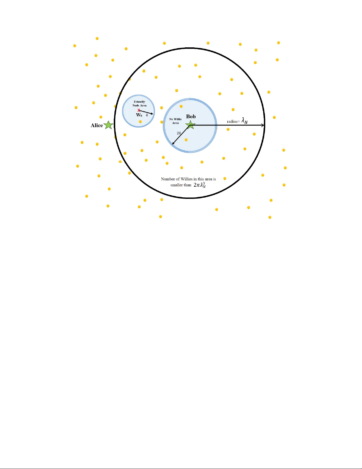
Co v ert W ireless Communication with Artiﬁcial Noise Generation Ramin Soltani, Member , IEEE, Dennis Goeckel, F ellow , IEEE, Don T owsle y , F ellow , IEEE, Boulat A. Bash, Member , IEEE, and Saikat Guha, Senior Member , IEEE Abstract Cov ert communication conceals the transmission of the message from an attentive adversary . Recent work on the limits of cov ert communication in additiv e white Gaussian noise (A WGN) channels has demonstrated that a covert transmitter (Alice) can reliably transmit a maximum of O ( √ n ) bits to a cov ert receiver (Bob) without being detected by an adversary (W arden W illie) in n channel uses. This paper focuses on the scenario where other “friendly” nodes distributed according to a two-dimensional Poisson point process with density m are present. W e propose a strategy where the friendly node closest to the adversary , without close coordination with Alice, produces artiﬁcial noise. W e show that this method allo ws Alice to reliably and covertly send O (min { n, m γ / 2 √ n } ) bits to Bob in n channel uses, where γ is the path-loss exponent. W e also consider a setting where there are N w collaborating adv ersaries uniformly and randomly located in the en vironment and show that in n channel uses, Alice can reliably and covertly send O  min n n, m γ / 2 √ n N γ w o bits to Bob when R. Soltani is with the Electrical and Computer Engineering Department, Univ ersity of Massachusetts, Amherst, MA (email: soltani@ecs.umass.edu). D. Goeckel is with the Electrical and Computer Engineering Department, Uni versity of Massachusetts, Amherst, MA (email: goeckel@ecs.umass.edu). D. T o wsley is with the College of Information and Computer Sciences, University of Massachusetts, Amherst, MA (email: towsle y@cs.umass.edu). B. Bash is with Raytheon BBN T echnologies, Cambridge, MA (email: boulat.bash@raytheon.com). S. Guha is with the College of Optical Sciences, Uni versity of Arizona, T ucson, AZ (email: saikat@email.arizona.edu). This work has been supported, in part, by the National Science Foundation under grants CNS-1018464, ECCS-1309573, and CNS- 1564067. The preliminary version of this work has been presented at the 52nd Annual Allerton Conference on Communication, Control, and Computing, Allerton, Monticello, IL, October 2014 [1]. c  2018 IEEE. Personal use of this material is permitted. Permission from IEEE must be obtained for all other uses, in any current or future media, including reprinting/republishing this material for advertising or promotional purposes, creating new collectiv e works, for resale or redistribution to servers or lists, or reuse of any copyrighted component of this work in other works. DOI: 10.1109/TWC.2018.2865946 1 γ > 2 , and O  min n n, m √ n N 2 w log 2 N w o when γ = 2 . Con versely , we demonstrate that no higher covert throughput is possible for γ > 2 . Keyw ords: Security and Priv acy , Co vert Communication, W ireless Communication, Artiﬁcial Noise Gen- eration, Cov ert W ireless Communication, Lo w Probability of Detection, LPD, Cov ert Channel, Covert W ireless Network, W ireless Network, Single-hop Communication, Additiv e White Gaussian Noise, A WGN, Information Theory , Covert Wireless Communication, Sensor Networks, Jamming, Capacity of Cov ert Channel, Capacity of W ireless Cov ert Communication. I . I N T RO D U C T I O N Cov ert communication hides the presence of a message from a watchful adversary . This is crucial in scenarios in which the standard method of secrecy , which hides the message content but not its existence, is not enough; in other words, there are applications where, no matter how strongly the message is protected from being deciphered, the adversary discerning that the communication is taking place results in penalties to the users. Examples of such scenarios include military operations, social unrest, and tracking of people’ s daily activities. The Snowden disclosures [2] demonstrate the utility of “meta-data” to an observing party and, thus, moti v ate hiding the presence of the message. The pro visioning of security and pri vac y has emer ged as a critical issue in communication systems [3]– [10]. In wireless communications where the signal is not restricted physically to a wire, it is more dif ﬁcult to hide the existence of the communication. Although spread spectrum approaches hav e been widely used in the past [11], the fundamental limits of cov ert communication were only recently established by a subset of the authors [12], [13], who presented a square root limit on the number of bits that can be transmitted securely from the transmitter (Alice) to the intended receiv er (Bob) when there is an additiv e white Gaussian noise (A WGN) channel between Alice and each of Bob and the adversary (W arden W illie). In particular , by taking advantage of positiv e noise po wer at W illie, Alice can reliably transmit O ( √ n ) bits to Bob in n channel uses while lower bounding W illie’ s error probability P (w) e = P F A + P MD 2 ≥ 1 2 −  for any 0 <  < 1 2 where P F A is the probability of false alarm and P MD is the probability of mis-detection. Con versely , if Alice transmits ω ( √ n ) bits in n uses of channel, either W illie detects her or Bob suffers a non-zero probability of decoding error as n goes to inﬁnity . Cov ert communications recently has been studied in many scenarios such as binary symmetric channels (BSCs) [14], multi-path noiseless networks [15], bosonic channels with thermal noise [16], and noisy discrete memoryless channels (DMCs) [17]. Furthermore, higher throughputs are achie vable when Alice can lev erage W illie’ s ignorance of her transmission time [18], and/or the adversary has uncertainty about channel characteristics [19]. These works, along with [20], [21], present a comprehensi ve characterization of the fundamental limits of co vert communications ov er DMC and A WGN channels and ha ve also 2 moti vated studying the fundamental limits of covert techniques for packet channels [22], [23] and in visible de-anonymization of network ﬂo ws [24]. In this paper , we take necessary steps to answer this question: what is the throughput of covert com- munication in wireless networks? In particular , we present a single-hop covert communication scheme which can be embedded into a large wireless network to extend the capacity of overt communication in large wireless networks [25], [26] to covert communication. The goal is to establish an analog to the line of work on scalable low probability of intercept communications [27]–[30], which considered the e xtension of [25], [26] to the secur e multipair unicast problem in lar ge wireless networks. Here, in analog to [13], we calculate the throughput of single-hop covert communication in the presence of a number of other network nodes: 1) warden W illies which decrease the throughout; 2) friendly nodes which can be employed to increase the throughput. In this paper , we enhance the throughout of co vert communication assuming that W illie knows his channel characteristics, as opposed to [19] where the throughput of the co vert communication is improved by le veraging W illie’ s ignorance of the channel characteristics in a fading en vironment or when a jammer with v arying po wer is present. Assume Alice attempts to communicate cov ertly with Bob without detection by W illie, but also in the presence of other (friendly) network nodes, which can assist the communication by producing background chatter to inhibit W illie’ s ability to detect Alice’ s transmission. W e model the locations of the friendly nodes by a two-dimensional Poisson point process of density m , and that Alice and Bob share a secret (codebook) unkno wn to W illie. For this scenario, described in more detail in Section II, we show in Section III that Alice is able to covertly transmit O (min { n, m γ / 2 √ n } ) bits to Bob in n channel uses while keeping Willie’ s error probability P (w) e ≥ 1 2 −  for any  ≥ 0 , where γ is the path-loss exponent. The construction that enables such a cov ert throughput is to switch on the closest friendly node to W illie. Conv ersely , without any restriction on the algorithm for turning on friendly nodes, we sho w that if Alice attempts to transmit ω ( m γ / 2 √ n ) bits to Bob in n channel uses, there exists a detector that W illie can use to either detect her with arbitrarily low error probability P (w) e or prev ent Bob from decoding the message with arbitrarily lo w probability of error . Next, we extend the scenario to the case where of multiple W illies, and we sho w that when N w collaborating Willies are uniformly and independently distributed in the unit box (see Fig. 1), we can still turn on the closest friendly node to each W illie to improve the co vert throughput. Ho wev er , as N w → ∞ , we observe two ef fects that reduce the cov ert throughput: (1) with high probability , there exists a Willie very close to Alice who receiv es a high signal power from her , thus making Alice employ a lo wer power to hide the transmission; (2) with high probability , there exists a W illie very close to Bob whose closest friendly node generates additional noise for Bob, hence reducing his ability to decode 3 Alice’ s message. W e explore this scenario in Section IV in detail. Finally , we discuss the results in Section V and present conclusions in Section VI. I I . S Y S T E M M O D E L , D E FI N I T I O N S , A N D M E T R I C S A. System Model Consider a source Alice ( A ) wishing to communicate with recei ver Bob ( B ) located a unit distance aw ay from her in the presence of adversaries (W arden W illies) W 1 , W 2 , . . . , W N w , who are distributed independently and uniformly in the unit square (Fig. 1) and seek to detect any transmission by Alice. When there is only a single W illie, we omit the subscript and denote it by W . Also present are friendly nodes F 1 , F 2 , . . . allied with Alice and Bob, who help hide Alice’ s transmission by generating noise. W e model the locations of friendly nodes by a two-dimensional Poisson point process with density m . The adv ersaries try to detect whether Alice transmits or not by processing the signals they receiv e and applying hypothesis testing on them, as discussed in the next subsection. W e consider two scenarios: a single W illie ( N w = 1 ) and multiple W illies ( N w > 1 ). W e assume all channels are discrete-time A WGN with real-valued symbols. Alice transmits n real-valued symbols s 1 , s 2 , . . . , s n that are samples of zero-mean Gaussian distribution with variance P a . Each friendly node is either on or off according to the strategy employed. Let θ j denote the state of the j th friendly node F j ; θ j = 1 if F j is “on” (transmits noise) and θ j = 0 (silent) otherwise. If F j is on, it transmits symbols n s ( j ) i o ∞ i =1 , where n s ( j ) i o ∞ i =1 is a collection of independent and identically distributed (i.i.d.) zero-mean Gaussian random variables, each with v ariance (power) P f . Denote by J the set of friendly nodes, and by J † the set of friendly nodes that are on. The locations of all the parties are static and known to everyone. One implication of this assumption is that friendly nodes can determine which friendly node is the closest to each W illie. Recalling that the distance between Alice and Bob is normalized to unity , Bob recei ves y (b) 1 , y (b) 2 , . . . , y ( b ) n where y (b) i = s i + z (b) i for 1 ≤ i ≤ n . The noise component is z (b) i = z (b) i, 0 + P ∞ j =1 θ j z (b) i,j , where n z (b) i, 0 o n i =1 is an i.i.d. sequence representing the background noise of Bob’ s receiv er with z (b) i, 0 ∼ N (0 , σ 2 b , 0 ) for all i , and n z (b) i,j o n i =1 is an i.i.d. sequence of zero-mean Gaussian random variables characterizing the chatter from the j th friendly node when it is “on”, each element of the sequence with variance P f d γ b , f j , where d x,y is the distance between nodes X and Y , and γ is the path-loss exponent which in most practical cases satisﬁes 2 ≤ γ ≤ 4 . Similarly , the k th W illie observes y ( k ) 1 , y ( k ) 2 , . . . , y ( k ) n where y ( k ) i = s i d γ / 2 a , w k + z ( k ) i . Here, z ( k ) i = z ( k ) i, 0 + P ∞ j =1 θ j z ( k ) i,j where n z ( k ) i, 0 o n i =1 is an i.i.d. sequence representing the background noise at W illie’ s receiv er , where z ( k ) i, 0 ∼ N (0 , σ 2 w k, 0 ) for all i , and n z ( k ) i,j o n i =1 is an i.i.d. sequence characterizing the chatter from the j th friendly node when it is “on”; thus, N (0 , P f /d γ w k , f j ) . For a single W illie scenario, we omit the 4 Fig. 1. System Conﬁguration: Source node Alice wishes to communicate reliably and without detection to the intended receiv er Bob at distance one (normalized) with the assistance of friendly nodes (represented by yellow nodes in the ﬁgure) distributed according to a two-dimensional Poisson point process with density m in the presence of adversary nodes W 1 , W 2 , . . . , W N w located in the dashed box ( N w = 3 in the ﬁgure). superscripts on y ( k ) i , z ( k ) i , and z ( k ) i,j , and we denote the W illie by W , and the closest friendly node to W illie by F . W e assume Alice and the friendly nodes, while ha ving a common goal, are not able to synchronize their transmissions; that is, the friendly nodes set up a constant power background chatter b ut are not able to, for example, lo wer their power at the time Alice transmits. In [19], the assumption is that a single jammer with varying po wer is present or the channel fading leads to uncertainty in W illie’ s recei ved po wer when Alice is not transmitting. Such uncertainty is not present here. In this paper , the density of friendly nodes m and the number of adversaries N W are functions of the number of channel uses n , and γ is a constant independent of n . B. Deﬁnitions W illie’ s hypotheses are H 0 (Alice does not transmit) and H 1 (Alice transmits). The parameters that determine W illie’ s error probabilities (type I and type II errors) are his distance to Alice d a , w and his noise po wer σ 2 w , which are random v ariables dependent on the locations of the friendly nodes and W illie(s). For 5 gi ven locations of the friendly nodes and Willie, we denote by P F A ( σ 2 w , d a , w ) the probability of rejecting H 0 when it is true (type I error or false alarm), and P MD ( σ 2 w , d a , w ) the probability of rejecting H 1 when it is true (type II error or mis-detection). Assuming equal prior probabilities, W illie’ s error prob- ability giv en the locations of friendly nodes and W illie(s) is P (w) e ( σ 2 w , d a , w ) = P F A ( σ 2 w ,d a , w )+ P MD ( σ 2 w ,d a , w ) 2 . W illie’ s type I error , type II error , and probability of error are P F A = E F , W [ P F A ( σ 2 w , d a , w )] , P MD = E F , W [ P MD ( σ 2 w , d a , w )] , and P (w) e = E F , W h P (w) e ( σ 2 w , d a , w ) i , respectiv ely , where E F , W [ · ] denotes the ex- pectation with respect to the locations of the friendly nodes as well as those of the W illie(s). W e assume that W illie uses classical hypothesis testing and seeks to minimize his probability of error , P (w) e . The generalization to arbitrarily prior probabilities is a v ailable in [13, Section V .B]. When there is only a single W illie in the scenario, he applies a hypothesis test to his receiv ed signal to determine whether or not Alice is communicating with Bob . For gi ven locations of the friendly nodes and W illie, we denote the probability distribution of W illie’ s ( W k ) collection of observations n y ( k ) i o n i =1 by P 1 ( σ 2 w , d a , w ) when Alice is communicating with Bob, and the distribution of the observ ations when she does not transmit by P 0 ( σ 2 w ) . For a scenario with multiple collaborating W illies (Theorems 2.1 and 2.2), they jointly process the signals the y receiv e to arriv e at a single collectiv e decision as to whether Alice transmits or not. In this case, we use P (w) e ( σ 2 w , d a , w ) , P F A ( σ 2 w , d a , w ) , P MD ( σ 2 w , d a , w ) , P 1 ( σ 2 w , d a , w ) , and P 0 ( σ 2 w ) , where σ 2 w and d a , w are vectors containing σ 2 w k and d a , w k , respecti vely . Deﬁnition 1. (Covertness) Alice’ s transmission is covert if and only if she can lower bound W illies’ probability of error ( P (w) e = E F , W h P (w) e ( σ 2 w , d a , w ) i = E F , W [ P F A ( σ 2 w ,d a , w )+ P MD ( σ 2 w ,d a , w ) ] 2 ) by 1 2 −  for an y  > 0 , asymptotically [13]. The expectation is with respect to the locations of the friendly nodes as well as those of the W illie(s). Bob’ s probability of error depends on his noise power σ 2 b which is a random v ariable dependent on the locations of W illie and friendly nodes. Denote by P (b) e ( σ 2 b ) Bob’ s probability of error for gi ven locations of the friendly nodes and W illie. Deﬁnition 2. (Reliability) Alice’ s transmission is reliable if and onl y if the desired recei ver (Bob) can decode her message with arbitrarily low probability of error P (b) e = E F , W h P (b) e ( σ 2 b ) i at long block lengths. In other words, for an y ζ > 0 , Bob can achiev e P (b) e < ζ as n → ∞ . In this paper, we use standard Big-O, Little-O, Big-Omega, Little-Omega, and Theta notations [31, Ch. 3]. 6 I I I . S I N G L E W A R D E N S C E N A R I O In this section, we consider the case where there is only one W illie ( W ) located uniformly and randomly on the unit square shown as a dashed box in Fig. 1. W e present Theorem 1.1 for γ > 2 in Section III-A, and Theorem 1.2 for γ = 2 in Section III-B. W e show that Alice is able to covertly transmit O (min { n, m γ / 2 √ n } ) bits to Bob in n channel uses. The construction that enables such a cov ert throughput is to turn on the closest friendly node to W illie to hide the presence of Alice’ s transmission. T o achie ve P (w) e ≥ 1 2 −  , Alice transmits codewords with power P a which depends on the covertness parameter  . The achiev ability proof concludes by considering the rate at which reliable decoding is still possible when Alice uses the maximum possible power . In Theorem 1.1, we present a conv erse independent of the status of the friendly nodes (being on or off), and in Theorem 1.2, we present a con verse assuming the closest friendly node to W illie is on. A. Single W arden Scenario and γ > 2 Theorem 1.1. When ther e is one war den (W illie) located randomly and uniformly over the unit square , m > 0 , and γ > 0 , Alice can reliably and co vertly tr ansmit O (min { n, m γ / 2 √ n } ) bits to Bob in n channel uses. Con versely , if Alice attempts to tr ansmit ω ( m γ / 2 √ n ) bits to Bob in n c hannel uses, there exists a detector that W illie can use to either detect her with arbitrarily low err or pr obability P (w) e or Bob cannot decode the messag e with arbitrarily low err or pr obability P (b) e . Proof. (Achie vability) Construction : Alice and Bob share a codebook that is not rev ealed to W illie. For each message transmission of length L bits, Alice uses a ne w codebook to encode the message into a codew ord of length n at rate R = L n . T o build a codebook, we use random coding arguments; that is, codew ords { C ( M l ) } 2 nR l =1 are associated with messages { M l } 2 nR l =1 , where each code word C ( M l ) = { C ( u ) ( M l ) } n u =1 , for l =  1 , 2 , · · · , 2 nR  , is an i.i.d. zero-mean Gaussian random sequence; that is, C ( u ) ( M l ) ∼ N (0 , P a ) where P a is speciﬁed later . Bob employs a maximum-likelihood (ML) decoder to process his observ ations { y ( b ) i } n i =1 [32]. The decoder picks a code word b C that maximizes P ( { y ( b ) i } n i =1 | b C ) , i.e., the probability that { y ( b ) i } n i =1 was recei ved, gi ven that b C was sent. Alice and Bob turn on the closest friendly node to W illie and keep all other friendly nodes off, whether Alice transmits or not. Therefore, W illie’ s observed noise po wer is giv en by σ 2 w = σ 2 w , 0 + P f d γ w , f , 7 where σ 2 w , 0 is W illie’ s noise power when none of the friendly nodes are transmitting and d w , f is the (random) distance between W illie and the closest friendly node to him; hence, σ 2 w is a random variable that depends on the locations of the friendly nodes. Analysis : ( Covertness ) First, we analyze W illie’ s error probability conditioned on σ 2 w and d a , w , P (w) e ( σ 2 w , d a , w ) , where d a , w is the distance between W illie to Alice. Then, we lower bound W illie’ s error probability P (w) e = E F , W [ P (b) e ( σ 2 w ) , d a , w ] . Recall that for giv en locations of the friendly nodes and W illie, P 0 ( σ 2 w ) is the joint probability density function (pdf) for W illie’ s observations under the null hypothesis H 0 (Alice does not transmit), and P 1 ( σ 2 w , d a , w ) be the joint pdf for corresponding observations under the hypothesis H 1 (Alice transmits). Observe P 0 ( σ 2 w ) = P n w ( σ 2 w ) , P 1 ( σ 2 w , d a , w ) = P n s ( σ 2 w , d a , w ) , where P w ( σ 2 w ) = N (0 , σ 2 w ) is the pdf for each of W illie’ s observ ations when Alice does not transmit, for gi ven locations of friendly nodes and W illie , and P s ( σ 2 w , d a , w ) = N  0 , σ 2 w + P a d γ a , w  is the pdf for each of the corresponding observ ations when Alice transmits. When W illie applies the optimal hypothesis test to minimize P (w) e ( σ 2 w , d a , w ) [13]: P (w) e ( σ 2 w , d a , w ) ≥ 1 2 − r 1 8 D ( P 1 ( σ 2 w , d a , w ) || P 0 ( σ 2 w )) , (1) where D ( f ( x ) || g ( x )) is the relative entropy between pdfs f ( x ) and g ( x ) . For the giv en P 0 and P 1 [13]: D ( P 1 ( σ 2 w , d a , w ) || P 0 ( σ 2 w )) = n 2  P a d γ a , w σ 2 w − ln  1 + P a d γ a , w σ 2 w  ≤ n  P a 2 d γ a , w σ 2 w  2 , (2) where the last inequality follo ws from (see the Appendix A) ln(1 + x ) ≥ x − x 2 2 , for x ≥ 0 . (3) By (1) and (2) P (w) e ( σ 2 w , d a , w ) ≥ 1 2 − r n 8 P a 2 σ 2 w d γ a , w . (4) If Alice sets her a verage symbol po wer P a ≤ cm γ / 2 √ n , (5) where c =   Γ( γ / 2+1) 4 √ 2 ψ γ P f π γ / 2+1  − 1 is a constant independent of n , Γ( · ) is the Gamma function, and ψ = p  2 π , then (4) yields P (w) e ( σ 2 w , d a , w ) ≥ 1 2 − r 1 8 cm γ / 2 2 σ 2 w d γ a , w . (6) 8 Denote by E F , W [ · ] the expectation ov er locations of the friendly nodes ( F 1 , F 2 , . . . ) , and the location of W illie ( W ). Next, we lo wer bound P (w) e = E F , W h P (w) e ( σ 2 w , d a , w ) i . Note that (6) contains a singu- larity at d a , w = 0 ; howe ver , since it occurs with probability measure zero, we can easily sho w that E F , W h 1 2 − q 1 8 cm γ / 2 2 σ 2 w d γ a , w i is bounded. Besides showing that E F , W h 1 2 − q 1 8 cm γ / 2 2 σ 2 w d γ a , w i is bounded, we need to show that the bound E F , W h 1 2 − q 1 8 cm γ / 2 2 σ 2 w d γ a , w i > 1 2 −  . T o do so, we deﬁne the ev ent d a , w > ψ and we sho w in Appendix B that E F , W  P (w) e ( σ 2 w , d a , w )   d a , w > ψ  ≥ 1 2 −  2 . (7) Then, applying the law of total e xpectation and the fact that P ( d a , w > ψ ) = 1 − π ψ 2 / 2 , we conclude P (w) e = E F , W [ P (w) e ( σ 2 w , d a , w )] ≥ E F , W  P (w) e ( σ 2 w , d a , w )   d a , w > ψ  P ( d a , w > ψ ) , ≥  1 2 −  2   1 − π ψ 2 2  =  1 2 −  2   1 −  4  > 1 2 − . (8) Thus, P (w) e > 1 2 −  for all  > 0 , as long as P a = O ( m γ / 2 √ n ) . Note that Alice does not use the locations of the friendly nodes nor the location of W illie to select the transmission power (and thus, per below , the corresponding rate). Rather , she selects a power and corresponding rate for a scheme that is co vert when a veraged o ver the locations of the friendly nodes. ( Reliability ) First, we analyze Bob’ s decoding error probability conditioned on σ 2 b = σ 2 b , 0 + P f d γ b , f , which we denote P (b) e ( σ 2 b ) , where d b , f is the distance from Bob to the friendly node closest to W illie. Then, we upper bound Bob’ s decoding error probability P (b) e = E F , W [ P (b) e ( σ 2 b )] . Bob’ s ML decoder results an error when a codeword b C other than the transmitted one maximizes P ( { y ( b ) i } n i =1 | b C ) . From an application of [13, Eqs. (5)-(9)], we can upper bound Bob’ s decoding error probability av eraged over all codebooks for a gi ven σ 2 b by: P (b) e  σ 2 b  ≤ 2 nR − n 2 log 2  1+ P a 2 σ 2 b  , (9) = 2 nR − n 2 log 2  1+ cm γ / 2 2 √ nσ 2 b  . (10) where the last step is obtained by having Alice set P a = cm γ / 2 √ n to satisfy (5). Let φ = q ln (2 / (2 − ζ )) mπ , where ζ > 0 is the reliability parameter (see Deﬁnition 2). Since the right hand side (RHS) of (10) is a monotonically non-decreasing function of d b , f , when d b , f > φ P (b) e  σ 2 b  ≤ 2 nR − n 2 log 2 1+ cm γ / 2 2 √ n ( σ 2 b , 0 + P f /φ γ ) ! . (11) W e set Alice’ s rate to R = min { 1 , R 0 } where R 0 = 1 4 log 2 1 + cm γ / 2 2 √ n  σ 2 b , 0 + P f /φ γ  ! . (12) 9 By (11), (12), P (b) e ( σ 2 b ) ≤ 2 n ( R − 2 R 0 ) . Note that R ≤ R 0 and thus R − 2 R 0 ≤ − R 0 . Consequently P (b) e  σ 2 b  ≤ 2 − nR 0 = 1 + cm γ / 2 2 √ n  σ 2 b , 0 + P f /φ γ  ! − n 4 ≤ 1 + cm γ / 2 √ n 8  σ 2 b , 0 + P f /φ γ  ! − 1 , (13) where (13) follo ws from the follo wing inequality provided n ≥ 4 (proved in the Appendix C) : (1 + x ) − r ≤ (1 + r x ) − 1 for any r ≥ 1 and x > − 1 . (14) Thus, E F , W [ P (b) e ( σ 2 b ) | d b , f > φ ] ≤ 1 + cm γ / 2 √ n 8( σ 2 b , 0 + P f /φ γ ) ! − 1 . (15) Next, we upper bound Bob’ s av erage decoding error probability P (b) e using (15). The law of total expectation yields P (b) e = E F , W [ P (b) e ( σ 2 b )] ≤ E F , W [ P (b) e ( σ 2 b ) | d b , f > φ ] + P ( d b , f ≤ φ ) . (16) Consider the ﬁrst term on the RHS of (16). By (15), lim n →∞ E F , W [ P (b) e ( σ 2 b ) | d b , f > φ ] = 0 . No w , consider the second term on the RHS of (16). Since the e vent { d b , f ≤ φ } is a subset of the ev ent that no friendly node is in the circle of radius φ centered at Bob, P ( d b , f ≤ φ ) ≤ 1 − e − mπ φ 2 = ζ / 2 , and thus lim n →∞ P (b) e ≤ ζ / 2 < ζ for any 0 < ζ < 1 . ( Number of Covert Bits ) Now , we calculate nR , the number of bits that Bob recei ves. By (12), if cm γ / 2 2 √ n ( σ 2 b , 0 + P f /φ γ ) ≥ 15 , then R 0 ≥ 1 , R = 1 , and thus nR = n . Now consider cm γ / 2 2 √ n ( σ 2 b , 0 + P f /φ γ ) < 15 . By (12), R 0 < 1 , and thus nR = n 4 log 2 1 + cm γ / 2 2 √ n  σ 2 b , 0 + P f /φ γ  ! . (17) Consequently , nR ≤ n 4 log 2 (1 + 15) = n . No w consider m = o ( n 1 /γ ) . Note that log 2 (1 + x ) ≤ x with equality when x = 0 . Therefore, nR = O ( m γ / 2 √ n ) . Thus, Bob receiv es O (min { n, m γ / 2 √ n } ) bits in n channel uses. ( Con verse ) W e present the con verse independent of the status (being on or off) of the friendly nodes. Recall that J † ⊂ J the set of friendly nodes that are on. Willie uses a po wer detector on his collection of observ ations { y i } n i =1 to form S = 1 n P n i =1 y 2 i and performs a hypothesis test based on S and a threshold t . If S < σ 2 w + t , W illie accepts H 0 (Alice does not transmit); otherwise, he accepts H 1 (Alice transmits). Recall that when H 0 is true, y i = z i, 0 + P ∞ f j ∈J † z i,j , where { z i, 0 } n i =1 is an i.i.d. sequence representing the background noise with z i, 0 ∼ N (0 , σ 2 w 1 , 0 ) , and { z i,j } n i =1 is an i.i.d. sequence characterizing the chatter from the j th friendly node with N (0 , P f /d γ w , f j ) . Since all of the sources of noise are independent, we can 10 model W illie’ s total noise by a Gaussian noise with y i ∼ N (0 , σ 2 w ) , where σ 2 w = σ 2 w , 0 + P f j ∈J † P f /d γ w , f j . Therefore [13, Eqs. (12),(13)], E Y [ S | H 0 ] = σ 2 w , V ar Y [ S | H 0 ] = 2 σ 4 w n , where E Y [ · ] and V ar Y [ · ] denote the expectation and variance with respect to W illie’ s receiv ed signal. When H 1 is true, Alice transmits a code word C ( M l ) =  C ( u ) ( M l )  n u =1 and W illie observes { y i } n i =1 which contains i.i.d. samples of mean shifted noise y i ∼ N  s i d γ / 2 a , w , σ 2 w  , where s i is the v alue of Alice’ s transmitted symbol in the i th channel use, and each s i is an instantiation of a Gaussian random variable N (0 , P a ) . Therefore [13, Eqs. (14),(15)], E Y [ S | H 1 ] = σ 2 w + P a d γ a , w , V ar Y [ S | H 1 ] = 4 P a d γ a , w σ 2 w + 2 σ 4 w n . W e show that Willie can choose the threshold t independent of locations of the friendly nodes, σ 2 w , and J † such that if Alice transmits ω  m γ / 2 √ n  bits to Bob, he can achie ve arbitrarily small average error probability . Bounding P F A ( σ 2 w , d a , w ) by using Chebyshe v’ s inequality yields [13]: P F A ( σ 2 w , d a , w ) ≤ 2 σ 4 w nt 2 . (18) Let η 1 = s ln  4 4 − λ  mπ . (19) Note that P F A = E F , W [ P F A ( σ 2 w , d a , w )] . By the law of total e xpectation: P F A = E F , W  P F A ( σ 2 w , d a , w )   d w , f ≤ η 1  P ( d w , f ≤ η 1 ) + E F , W  P F A ( σ 2 w , d a , w )   d w , f > η 1  P ( d w , f > η 1 ) , ≤ P ( d w , f ≤ η 1 ) + E F , W  P F A ( σ 2 w , d a , w )   d w , f > η 1  , =  1 − e − mπ η 2 1  + E F , W  P F A ( σ 2 w , d a , w )   d w , f > η 1  , ( a ) = λ 4 + E F , W  P F A ( σ 2 w , d a , w )   d w , f > η 1  = λ 4 + 2 nt 2 E F , W  σ 4 w | d w , f > η 1  , (20) where ( a ) follows from (19), and the last step follows from (18). Let σ 2 w ( r ) be W illie’ s noise power considering only the friendly nodes in the circle of radius r > η 1 centered at W illie, and N f be the (random) number of friendly nodes in the area surrounded by the circles of radii η 1 and r centered at W illie. Then: σ 2 w ( r ) = σ 2 w , 0 + P f X η 1 η 1  ≤ σ 4 w , 0 + 2 P f mπ r 2 σ 2 w , 0 E F [1 /d γ w , f i | d w , f > η 1 ] + P 2 f mπ r 2 E F [1 /d 2 γ w , f i | d w , f > η 1 ] , + P 2 f m 2 π 2 r 4 E F [1 /d γ w , f i | d w , f > η 1 ] 2 , (22) and in Appendix E that for lar ge enough n : E F [1 /d γ w , f i | d w , f > η 1 ] ≤ 4 γ − 2 η 2 − γ 1 r 2 , (23) E F [1 /d 2 γ w , f i | d w , f > η 1 ] ≤ 2 γ − 1 η 2 − 2 γ 1 r 2 . (24) Since η 1 = Θ( m − 1 / 2 ) , (23), (24), the ﬁrst four terms on the RHS of (22) are O (1) , O ( m γ / 2 ) , O ( m γ ) and O ( m γ ) , respecti vely . Consequently , for large enough n : E F , W  σ 4 w ( r ) | d w , f > η 1  ≤ ρ 2 m γ , (25) where ρ = 2 π γ / 2 P f s min {  ln  4 4 − λ  1 − γ , 8  ln  4 4 − λ  2 − γ } γ − 1 . (26) This means that the noise generated by the closest friendly node to W illie dominates the noise generated from other friendly nodes. By (25), σ 4 w ( r 1 ) ≤ σ 4 w ( r 2 ) for η 1 ≤ r 1 ≤ r 2 . Therefore, the monotone con vergence theorem yields: E F , W  σ 4 w | d w , f > η 1  ≤ ρ 2 m γ . (27) Let W illie choose threshold t = √ 8 ρm γ / 2 √ nλ . By (20), P F A ≤ λ 4 + λ 4 = λ 2 . (28) Next, we upper bound P MD = E F , W [ P MD ( σ 2 w , d a , w )] . Since d a , w ≤ 2 , W illie can achiev e [13, Eq. (16)] P MD ( σ 2 w , d a , w ) ≤ 4 P a d γ a , w σ 2 w + 2 σ 4 w n  P a d γ a , w − t  2 = 4 P a d γ a , w σ 2 w + 2 σ 4 w n  P a 2 γ − t  2 . (29) 12 Let η 2 = q ln ( 4 4 − λ + λ 0 ) mπ , where 0 < λ 0 < λ , and η 3 = q λ 2 π . The law of total e xpectation yields P MD ≤ P ( { d w , f ≤ η 2 } ∪ { d a , w ≤ η 3 } ) + E F , W  P MD ( σ 2 w , d a , w )   { d w , f > η 2 } ∩ { d a , w > η 3 }  , ( b ) ≤  1 − e − mπ η 2 2  + π 2 η 2 3 + E F , W  P MD ( σ 2 w , d a , w )   { d w , f > η 2 } ∩ { d a , w > η 3 }  , ( c ) = λ − λ 0 4 + λ 4 + E F , W  P MD ( σ 2 w , d a , w )   { d w , f > η 2 } ∩ { d a , w > η 3 }  , ≤ λ − λ 0 4 + λ 4 + 4 P a η γ 3 E F , W [ σ 2 w | d w , f > η 2 ] n  P a 2 γ − t  2 + 2 E F , W [ σ 4 w | d w , f > η 2 ] n  P a 2 γ − t  2 , (30) where ( b ) follo ws from the union bound, ( c ) follo ws from substituting the v alues of η 2 and η 3 , and the last step follows from taking the conditional expectation of (29) giv en { d w , f ≤ η 2 } ∪ { d a , w ≤ η 3 } and upper bounding 1 /d γ a , w by 1 /η γ 3 . Consider E F , W [ σ 2 w | d w , f > η 2 ] and E F , W [ σ 4 w | d w , f > η 2 ] in (30). Similar to the ar guments leading to (27), we sho w that E F , W [ σ 4 w | d w , f > η 2 ] = O ( m γ ) . Consequently , Jensen’ s inequality yields E F , W [ σ 2 w | d w , f > η 2 ] = O ( m γ / 2 ) . In addition, t = Θ  m γ / 2 √ n  . Thus, if Alice sets her a verage symbol power P a = ω  m γ / 2 √ n  , then there exists n 0 > 0 s.t. ∀ n > n 0 ( λ 0 ) E F , W [ P MD ] ≤ λ − λ 0 4 + λ 4 + λ 0 2 = λ 2 + λ 0 4 < λ. (31) By (28) and (31), for any λ > 0 P (w) e = P F A + P MD 2 ≤ 3 λ 4 < λ. Consequently , Alice cannot send any codeword with av erage symbol po wer ω  m γ / 2 √ n  cov ertly . Thus, to a void detection of a gi ven codeword, she must set the power of that codew ord to P U = O  m γ / 2 √ n  . Suppose that Alice’ s codebook contains a fraction ξ > 0 of codew ords with po wer P U = O  m γ / 2 √ n  . For such low power codew ords, we can lower bound Bob’ s decoding error probability giv en the locations of the friendly nodes by [13, Eq. (20)] P U e ( σ 2 b ) ≥ 1 − P U 2 σ 2 b + 1 n log 2 ξ n + R ≥ 1 − P U 2 σ 2 b , 0 + 1 n log 2 ξ n + R . (32) Since Alice’ s rate is R = ω  m γ / 2 √ n  bits/symbol, P U e ( σ 2 b ) is bounded aw ay from zero as n → ∞ .  B. Single W arden Scenario and γ = 2 Theorem 1.2. When ther e is one war den (W illie) located randomly and uniformly over the unit square , m > 0 , and γ = 2 , Alice can r eliably and covertly transmit O (min { n, m √ n } ) bits to Bob in n channel uses. Con versely , if only the closest friendly node to W illie is on and Alice attempts to transmit 13 ω ( m γ / 2 √ n ) bits to Bob in n channel uses, ther e exists a detector that W illie can use to either detect her with arbitrarily low err or pr obability P (w) e or Bob cannot decode the messag e with arbitrarily low err or pr obability P (b) e . Proof. (Achie vability) The achiev ability (construction and analysis) is the same as that of 1.1. ( Con verse ) For γ > 2 , we upper bounded W illie’ s noise by the recei ved noise power in the worst case scenario where all of the friendly nodes are on, and it was optimal since σ 2 w = O ( m γ / 2 ) . Howe ver , for γ = 2 , noise po wer for the worst case scenario is O ( m log( m )) which is not optimal. W e assume only the closest friendly node to W illie is on and W illie knows that. The proof fol- lo ws from that of γ > 2 with modiﬁcations of (20) and (30), noting that E F , W [ σ 4 w | d w , f > η 1 ] = E F , W  ( σ 2 w 0 + P f /d γ w , f ) 2 | d w , f > η 1  ≤ ( σ 2 w 0 + P f /η γ 1 ) 2 .  I V . M U L T I P L E C O L L A B O R A T I N G W A R D E N S S C E N A R I O In this section, we consider the case when there are N w collaborating W illies located independently and uniformly in the unit square (see Fig. 1). W e present Theorem 2.1 for γ > 2 in Section IV -A, and Theorem 2.2 for γ = 2 in Section IV -B. Analogous to the single warden scenario, Alice and Bob’ s strategy is to turn on the closest friendly node to each W illie and keep all other friendly nodes off, whether Alice transmits or not. A. γ > 2 Theorem 2.1. When friendly nodes are independently distrib uted according to a two-dimensional P oisson point pr ocess with density m = ω (1) , and N w = o ( m/ log m ) collabor ating W illies ar e uniformly and independently distributed over the unit squar e shown in F ig. 1, then Alice can r eliably and covertly transmit O  min n n, m γ / 2 √ n N γ w o bits to Bob in n channel uses. Con versely , if only the closest friendly node to each W illie is on and Alice attempts to transmit ω  √ nm γ / 2 N γ w  bits to Bob in n c hannel uses, ther e exists a detector that W illie can use to either detect her with arbitrarily low err or pr obability P (w) e or Bob cannot decode the messag e with arbitrarily low err or pr obability P (b) e . W e present the proof assuming N w = ω (1) , as the proof for a ﬁnite N w follo ws from it. In addition, according to the statement of Theorem 2.1, if N w = Ω  n 1 2 γ √ m  , then Alice can reliably and covertly transmit O (1) bits to Bob in n uses of channel, which is not of interest. Therefore, we present the proof assuming N w = o  min n m log m , n 1 2 γ √ m o . Proof. (Achie vability) 14 Construction: The construction and Bob’ s decoding are the same as those of Theorems 1.1 and 1.2. Analysis: ( Covertness ) By (1), when W illie applies the optimal hypothesis test to minimize his error probability , P (w) e ( σ 2 w , d a , w ) ≥ 1 2 − r 1 8 D ( P 1 ( σ 2 w , d a , w ) || P 0 ( σ 2 w )) . (33) Here, σ 2 w and d a , w are vectors containing σ 2 w k and d a , w k , respectiv ely , P 0 ( σ 2 w ) = Q n i =1 P 0 ,i ( σ 2 w ) and P 1 ( σ 2 w , d a , w ) = Q n i =1 P 1 ,i ( σ 2 w , d a , w ) are the joint probability distributions of the W illies’ chan- nels observ ations for the H 0 and H 1 hypotheses, respectiv ely , where P 0 ,i ( σ 2 w ) = Q N w k =1 P ( k ) w k ( σ 2 w k ) and P 1 ,i ( σ 2 w , d a , w ) are the joint probability distrib ution of the i th channel observ ation of the W illies for H 0 and H 1 hypotheses, respectiv ely . The relativ e entropy between two multi variate normal distributions P 1 ( σ 2 w , d a , w ) and P 0 ( σ 2 w ) is [33]: D ( P 1 ( σ 2 w , d a , w ) || P 0 ( σ 2 w )) = 1 2  tr  Σ − 1 0 Σ 1  + ( µ 0 − µ 1 ) > Σ − 1 0 ( µ 0 − µ 1 ) − dim (Σ 0 ) − ln  | Σ 1 | | Σ 0 |  , (34) where tr( · ) , | · | , and dim( · ) denote the trace, determinant and dimension of a square matrix respectiv ely , µ 0 = 0 , µ 1 = 0 are the mean vectors, and Σ 0 , Σ 1 are nonsingular cov ariance matrices of P 0 ( σ 2 w ) and P 1 ( σ 2 w , d a , w ) , respecti vely , gi ven by Σ 0 = S ⊗ I n × n , Σ 1 =  S + P a U U T  ⊗ I n × n , where S = diag ( σ 2 w 1 , . . . , σ 2 w N w ) , ⊗ denotes the Kronecker product between two matrices, I n × n is the identity matrix of size n , and U is a column vector of size N w gi ven by U = h 1 /d γ / 2 a , w 1 1 /d γ / 2 a , w 2 . . . 1 /d γ / 2 a , w N w i T . Next, we calculate the relati ve entropy in (34). The ﬁrst term on the RHS of (34) is: tr  Σ − 1 0 Σ 1  = n N w X k =1 1 σ 2 w k  σ 2 w k + P a d γ a , w k  = nN w + n N w X k =1 P a d γ a , w k σ 2 w k . Then, | Σ 0 | = | S ⊗ I n × n | ( d ) = | S | n | I n × n | N w = | S | n = N w Y k =1 σ 2 w k ! n . where ( d ) is true from the determinant of the Kronecker product property presented in [34, p. 279]. Because σ 2 w k > 0 , S is nonsingular . Therefore, | Σ 1 | =   S + P a U U T   n | I n × n | N w =   S + P a U U T   n = | S | n   I + P a S − 1 U U T   n ( e ) = | S | n  1 + P a U T S − 1 U  n , = | Σ 0 | 1 + N w X k =1 P a d γ a , w k σ 2 w k ! n , 15 where ( e ) is due to Lemma 1.1 in [35]. Therefore, ln  | Σ 1 | | Σ 0 |  = n ln 1 + N w X k =1 P a d γ a , w k σ 2 w k ! . Thus, D ( P 1 ( σ 2 w , d a , w ) || P 0 ( σ 2 w )) = n 2 N w X k =1 P a d γ a , w k σ 2 w k − ln 1 + N w X k =1 P a d γ a , w k σ 2 w k !! . (35) Suppose Alice sets her a verage symbol po wer so that P a ≤ cm γ / 2 √ nN γ / 2 w , (36) where c = P f  γ / 2 ( γ − 2) π γ / 2 2 γ − 0 . 5 Γ ( γ / 2 + 1) . (37) By (3) and (35), D ( P 1 ( σ 2 w , d a , w ) || P 0 ( σ 2 w )) ≤ n 4 N w X k =1 P a d γ a , w k σ 2 w k ! 2 ≤ c 2 m γ 4 N γ w N w X k =1 1 d γ a , w k σ 2 w k ! 2 . (38) where the last step follo ws from (36). Similar to the ar guments leading to (8), to achiev e P (w) e > 1 2 −  , we deﬁne the e vent (see Fig. 2) A = N w \ i =1 { d a , w k > κ } , which occurs when all of the W illies are outside of the semicircular region with radius κ = p  4 N w around Alice. Then, we sho w in Appendix F that for any  > 0 Alice can achiev e: E F , W  P (w) e ( σ 2 w , d a , w )   A ] ≥ 1 2 (1 −  ) . (39) Next, we sho w that since κ < 1 / 2 , P ( A ) =  1 − π κ 2 2  N w ( f ) ≥ 1 − π N w κ 2 2 ≥ 1 − 2 N w κ 2 = 1 −  2 , (40) where ( f ) is true since (14) is true. By (39), (40), and the law of total expectation P (w) e = E F , W [ P (w) e ( σ 2 w , d a , w )] ≥ E F , W  P (w) e ( σ 2 w , d a , w )   A  P ( A ) =  1 2 −  2   1 −  2  ≥ 1 2 − , and thus communication is cov ert as long as P a = O  m γ / 2 √ nN γ / 2 w  . ( Reliability ) Next, we calculate the number of bits that Alice can send to Bob co vertly and reliably . Consider arbitrarily ζ > 0 . W e show that Bob can achie ve P (b) e < ζ as n → ∞ , where P (b) e is Bob’ s ML decoding error probability averaged over all possible codewords and the locations of friendly nodes 16 Fig. 2. Event A is true when there is no W illie in the semicircular region with radius κ shown above. Alice is only able to communicate cov ertly with intended receiv er Bob if A is true. and W illies. Bob’ s noise power is σ 2 b ≤ σ 2 b , 0 + P N w k =1 P f d γ b , f k , where d b , f k is the distance between Bob and the closest friendly node to the k th W illie ( W k ), and the inequality becomes equality when each W illie has a distinct closest friendly node. By (9) and (36), P (b) e  σ 2 b  ≤ 2 nR − n 2 log 2 1+ cm γ / 2 2 √ nσ 2 b N γ / 2 w ! . (41) Suppose Alice sets R = min { R 0 , 1 } , where R 0 = 1 4 log 2  1 + c 0 m γ / 2 4 N γ w √ n  , (42) c 0 = c ζ γ / 2 − 1 ( γ − 2) 2 γ +3 P f π γ / 2 , and c is deﬁned in (37). By the la w of total expectation, P (b) e = E F , W [ P (b) e  σ 2 b  ] ≤ E F , W  P (b) e  σ 2 b     c 0 σ 2 b cN γ / 2 w ≤ 1  + P  c 0 σ 2 b cN γ / 2 w > 1  . (43) Consider the ﬁrst term on the RHS of (43). W e show in Appendix G that since m = ω (1) , N w = ω (1) , and N w = o  n 1 2 γ √ m  , lim n →∞ E F , W  P (b) e  σ 2 b     c 0 σ 2 b cN γ / 2 w ≤ 1  = 0 . (44) 17 Fig. 3. Event B is true when there is no Willie in the semicircular region with radius 2 δ around Bob, and the distance between each W illie and the closest friendly node to him is smaller than δ , i.e., { 2 d w k , f k ≤ δ } ∩ { d b , w k > 2 δ } for 1 ≤ k ≤ N w . Consider the second term on the RHS of (43). T o upper bound P  c 0 σ 2 b cN γ / 2 w > 1  , we deﬁne the e vent B = N w \ k =1 {{ d w k , f k ≤ δ } ∩ { d b , w k > 2 δ }} , where δ = q ζ 4 π N w . This e vent occurs when there is no W illie in the semicircular re gion with radius 2 δ around Bob, and the distance between each W illie and the closest friendly node to him is smaller than δ (see Fig. 3). The law of total probability yields P  c 0 σ 2 b cN γ / 2 w > 1  ≤ P  c 0 σ 2 b cN γ / 2 w > 1     B  + P  ¯ B  . W e sho w in Appendix H that since N w = ω (1) , lim n →∞ P  c 0 σ 2 b cN γ / 2 w > 1     B  = 0 , (45) and in Appendix I that since N w = ω (1) and N w = o ( m/ log m ) , lim n →∞ P  ¯ B  = ζ / 2 . (46) Thus, (43)-(46) yield lim n →∞ P (b) e < ζ for an y 0 < ζ < 1 . 18 ( Number of Covert Bits ) Similar to the analysis of Theorem 1.1, we can show that when γ > 2 , Bob recei ves O  min n n, m γ / 2 √ n N γ w o bits in n channel uses. (Con verse) W e present the con verse assuming that the closest friendly node to each W illie is on and the W illies kno w this. W e sho w that the signal recei ved by the closest Willie to Alice is suf ﬁcient to detect Alice’ s communication. Intuitiv ely , the W illie closest to Alice has the best signal-to-noise ratio (SNR) and is the best W illie to detect Alice’ s communication. Denote W illie with minimum distance to Alice by W 1 . W e assume that W 1 kno ws σ 2 w 1 and the jamming scheme, in particular the distance between the closest friendly node to him and its transmit po wer . W 1 uses a po wer detector on his collection of observ ations n y (1) i o n i =1 to form S = 1 n P n i =1  y (1) i  2 , picks a threshold t , and performs a hypothesis test based on S . If S < σ 2 w 1 + t , he chooses H 0 (Alice does not transmit), otherwise, H 1 (Alice transmits). Observe σ 2 w 1 ≤ σ 2 w 1 , 0 + N w X k =1 P f d γ w 1 , f k , (47) where σ 2 w 1 , 0 is W illie’ s noise power when all of the friendly nodes are off, i.e., A WGN, and d w 1 , f k is the distance between W 1 and the closest friendly node to W k . Note that (47) becomes equality when all of the W illies ha ve a distinct closest friendly node. Similar to the con verse in Theorem 1.1, we sho w that E Y [ S | H 0 ] = σ 2 w 1 , (48) V ar Y [ S | H 0 ] = 2 σ 4 w 1 n , (49) E Y [ S | H 1 ] = σ 2 w 1 + P a d γ a , w 1 , (50) V ar Y [ S | H 1 ] = 4 P a σ 2 w 1 nd γ a , w 1 + 2 σ 4 w 1 n . (51) If S < σ 2 w 1 + t , W 1 accepts H 0 ; otherwise, he accepts H 1 . In the con verse of Theorem 1.1 we upper bounded W illie’ s noise power by the receiv ed noise power when all of the friendly nodes are on. Similar to the arguments leading to (28) we sho w that if we choose t = √ 8 ρm γ / 2 √ nλ , where ρ is giv en in (26), then: P F A ≤ λ 2 . (52) No w , consider P MD ( σ 2 w , d a , w ) . Similar to the approach leading to (29), we obtain P MD ( σ 2 w , d a , w ) ≤ 4 P a d γ a , w 1 σ 2 w 1 + 2 σ 4 w 1 n  P a d γ a , w 1 − t  2 . (53) 19 Deﬁne the e vent E = { d w 1 ,f 1 > η 1 } ∩ { `β 0 ≤ d a , w 1 < β 0 } , where η 1 is deﬁned in (19), and β 0 = p 2 ln (8 /λ ) / ( π N w ) , ` = p ln (1 − λ/ 8) / ln ( λ/ 8) . (54) The law of total e xpectation yields P MD = E F , W [ P MD ( σ 2 w , d a , w )] ≤ E F , W  P MD ( σ 2 w , d a , w )   E  + P ( E ) . (55) W e sho w in Appendix J since m = ω (1) , and N w = ω (1) , lim n →∞ P ( E ) ≤ λ/ 2 , (56) and, in Appendix K that E F , W  P MD ( σ 2 w , d a , w )   E  ≤ 4 P a ( `β 0 ) γ E F , W [ σ 2 w 1 | d w 1 ,f 1 > η 1 ] n  P a β 0 γ − t  2 + 2 E F , W [ σ 4 w 1 | d w 1 ,f 1 > η 1 ] n  P a β 0 γ − t  2 , (57) Consider E F , W  σ 2 w 1 | d w 1 , f 1 > η 1  and E F , W  σ 4 w 1 | d w 1 , f 1 > η 1  in (30). Similar to the arguments lead- ing to (27), we show that E F , W  σ 4 w 1 | d w 1 , f 1 > η 1  = O ( m γ ) . Consequently , Jensen’ s inequality yields E F , W  σ 2 w 1 | d w 1 , f 1 > η 1  = O ( m γ / 2 ) . Since t = Θ( m γ / 2 / √ n ) , β 0 = Θ(1 / √ N w ) , m = ω (1) , and N w = ω (1) , if Alice sets her av erage symbol po wer P a = ω  m γ / 2 √ nN γ / 2 w  , E F , W [ P MD ( σ 2 w , d a , w ) |E ] = 0 as n → ∞ . By (55) and (56) lim n →∞ P MD ≤ λ/ 2 . (58) Combined with (52), P F A + P MD ≤ λ for any λ > 0 . Thus, to a void detection for a giv en code word, Alice must set the po wer of that codeword to P U = O  m γ / 2 √ nN γ / 2 w  . Suppose that Alice’ s codebook contains a fraction ξ > 0 of code words with power P U = O  m γ / 2 √ nN γ / 2 w  . Similar to con verse of Theorem 1.1, gi ven the locations of the friendly nodes, Bob’ s decoding error probability of such lo w po wer codew ords is lo wer bounded by (see (32)) P U e ( σ 2 b ) ≥ 1 − P U 2 σ 2 b + 1 n log 2 ξ n + R . Denote the closest W illie to Bob by W 2 . Since Bob’ s noise is lower bounded by the noise generated from the closest friendly node to W 2 , σ 2 b ≥ P f d γ b , f 2 , P U e ( σ 2 b ) ≥ 1 − P U d γ b , f 2 2 P f + 1 n log 2 ξ n + R . 20 Deﬁne the ev ent F = n d b , f 2 < p 8 ln (1 /τ ) / ( π N w ) o , where 0 < τ < 1 . The law of total expectation yields P U e = E F , W  P U e ( σ 2 b )  ≥ E F , W  P U e ( σ 2 b )   F  P ( F ) . (59) Consider P ( F ) . W e show in Appendix L that since m = ω (1) , N w = ω (1) , and N w = o ( m/ log m ) , lim n →∞ P ( F ) = 1 − τ . (60) No w , consider E F , W  P U e   F  in (59). E F , W  P U e ( σ 2 b )   F  ≥ 1 − E F , W   P U d γ b , f 2 2 P f + 1 n log 2 ξ n + R       F   ( g ) ≥ 1 − E F , W     P U  2 π ln 1 τ √ N w  γ 2 P f + 1 n log 2 ξ n + R         F     , = 1 − E F , W    P U N γ / 2 w ( 2 π ln 1 τ ) γ 2 P f + 1 n log 2 ξ n + R        F    , where ( g ) is true since F occurs. Suppose Alice desires to transmit ω  √ nm γ / 2 N γ w  cov ert bits in n channel uses. Therefore, her rate (bits/symbol) is R = ω  m γ / 2 √ nN γ w  . Since P U = O  m γ / 2 √ nN γ / 2 w  , m = ω (1) , and N w = ω (1) , lim n →∞ E F , W  P U e ( σ 2 b )   F  = 1 . (61) By (59), (60), and (61), for any 0 < τ < 1 , lim n →∞ P U e ≥ 1 − τ , and thus E  P U e  is bounded away from zero.  B. γ = 2 Theorem 2.2. When friendly nodes ar e independently distributed according to a two-dimensional P ois- son point pr ocess with density m = ω (1) , and N w collaborating W illies ar e uniformly and independently distributed over the unit squar e shown in F ig. 1. If N w = o ( m/ log m ) , then Alice can r eliably and covertly tr ansmit O  min n n, m √ n N 2 w log 2 N w o bits to Bob in n channel uses. W e present the proof assuming N w = ω (1) , as the proof for a ﬁnite N w follo ws from it. In addition, according to the statement of Theorem 2.2, N w = Ω  m √ n log ( m √ n )  then Alice can reliably and covertly transmit O (1) bits to Bob in n uses of channel, which is not of interest. Therefore, we present the proof assuming N w = o  min n m log m , m √ n log ( m √ n ) o . Proof. (Achie vability) Construction: The construction and Bob’ s decoding are the same as those of Theorem 2.1. 21 Analysis: ( Covertness ) The difference between the results for γ > 2 and γ = 2 originates from the follo wing integral necessary in the proofs: Z dx x γ − 1 =      x 2 − γ / (2 − γ ) + c 0 , γ > 2 ln x + c 0 0 , γ = 2 , where c 0 and c 0 0 are constants. Therefore, the analysis for γ = 2 follows similarly with a fe w minor modiﬁcations. Alice sets her a verage symbol po wer P a ≤ cm √ nN w ln N w where c = 4 √ 2 π P f . (62) Next, we modify (78) to E W h 1 d 2 a , w k    d a , w k > κ i ≤ π ln ( N w ) . Then, we sho w that Alice achie ves (39) and thus her communication is cov ert as long as P a = O  m √ nN w log N w  . ( Reliability ) Similar to the approach in the reliability for γ > 2 , we can show that if Alice sets R = min { 1 , R 0 } , where R 0 = 1 4 log 2  1 + c 0 m 4 N 2 w (ln N w ) 2 √ n  , (63) c 0 = c 8 π P f , and c is deﬁned in (62), then m = ω (1) , N w = ω (1) , and N w = o  min n m log m , m √ n log ( m √ n ) o yield lim n →∞ P b e < ζ for an y 0 < ζ < 1 . ( Number of Covert Bits ) Similar to the analysis for γ > 2 , by (63), Bob receiv es O  min n n, m γ / 2 √ n N 2 w log 2 N w o bits in n channel uses.  ( Con verse ) The approach used for γ > 2 , which in volv ed choosing the closest W illie to Alice to decide whether Alice communicates with Bob or not, does not yield a tight result for γ = 2 . Using this approach, we can show that if Alice sets her av erage symbol po wer P a = ω  m √ nN w  , then W illie detects her with arbitrarily small sum of error probabilities. Ho wev er , from the achiev ability , we e xpect that P a = ω  m √ nN w log N w  results in detection. This suggests that W illies hav e to consider their signals recei ved collectiv ely to detect Alice’ s communication, as we expect for γ = 2 the signal decays slo wly with distance. V . D I S C U S S I O N A. Assumption of m = ω (1) in Theorems 2.1 and 2.2 In Theorems 2.1 and 2.2, we assumed m = ω (1) in order to simplify the proof when N w = ω (1) , but this condition can be relax ed. When relaxing this assumption, we also ha ve to replace the condition N w = o ( m/ log m ) with N w ≤ mζ 4 log ( mζ / 4) . Furthermore, m = ω (1) becomes plausible when the single-hop 22 communication scheme presented in this paper is extended to the cov ert multi-hop communication ov er large wireless netw orks [25], [26] where a collection of nodes w ork to establish co vert communication between a collection of source and destination pairs. In this case, the number of nodes often gro ws in the region of a single hop of communication [28], [36] with the size of the network [25], [26], [37], [38]. Note that we hav e allo wed a gro wing number of nodes for both friendly nodes ( m = ω (1) ) and warden W illies ( N w = ω (1)) . An e xample of employing artiﬁcial noise generation with a gro wing density of nodes in a lar ge wireless network is presented in [28], where authors analyze the throughput of ke y-less secure communication in a cell of size √ n × √ n and exploit the dynamics of wireless fading channels to achiev e secret communication. In particular , transmitter and recei ver nodes are distributed according to a Poisson point process with density one in the cell, and each node is allo wed to generate artiﬁcial noise. B. Assumption of turning on only the closest friendly node to each W illie For the achiev ability proofs in this paper , our strategy was turning on the closest friendly node to each W illie and keeping other friendly nodes off. For the case of a single Willie and γ > 2 , the con verse of Theorem 1.1, which is done over all strate gies for turning on the friendly nodes, shows that this was indeed an optimal strate gy . Howe ver , for the con verses of Theorems 1.2 and 2.1, we had to restrict ourselves to considering only those strategies that turn on the closest friendly node to each W illie. Whereas this is a limitation of that con verse, it is likely that this strate gy is either optimal or close to optimal in practice. In particular , in [39], [40], the authors propose that this strategy is optimal in wireless communication when the jammers (friendly nodes) hav e the same ﬁnite power , and using simulations they sho w that the noise receiv ed from other nodes (second closest node, third closest node, ...) is negligible compared to the noise receiv ed from the nearest jammer (friendly node). The optimality of this strategy is also addressed in [36]. Switching on only the closest node to Willie(s) requires knowing the location of W illie(s), col- laboration between friendly nodes, and switching of f a large number of friendly nodes, which might entail a high cost. Ho wev er, gi ven the importance of covert communication and the demand for it in speciﬁc applications (e.g., military), it is reasonable to pay the cost in these applications to increase the throughput of covert communication to a throughput higher than O ( √ n ) bits in n channel uses [13]. In addition to the this strategy , here we discuss an alternativ e strategy without these requirements: we only turn off the friendly nodes whose distances to Bob are smaller than ι > 0 , and we assume that other friendly nodes are on, independently , with probability p > 0 , where ι and p are independent of m, n, N W . Compared to our previous strategy , E F [1 /σ 2 w ] = O ( m − γ / 2 ) remains the same; howe ver , the 23 conjecture is that E F [ σ 2 b ] changes from O (1) to O ( m ) , and that Alice can reliably and cov ertly transmit O (min { n, m γ / 2 − 1 √ n } ) bits to Bob in n channel uses. Also, it is a conjecture that for a scenario with multiple W illies provided γ > 2 , Alice can reliably and co vertly transmit O  min n n, m γ / 2 − 1 √ n N γ w o bits to Bob in n channel uses. C. High pr obability r esults In this paper , our covertness metric (see Deﬁnition 1) requires lower bounding the e xpected value of W illies’ probability of error ( P (w) e ) o ver all instantiations of the locations of W illies and friendly nodes, by 1 2 −  for all  . In Appendix M, we present an example of the high probability result for the cov ertness of the single W illie scenario. D. Assumption of uniform distribution for W illies For spatial modeling of wireless networks, a Poisson point process is the most common choice [41]– [43]. When a Poisson point process is conditioned on the number of points in an area, the locations of the points in that area become uniformly distributed. In this paper , our goal was to ﬁrst consider the case of a single W illie and then extend the results to multiple W illies. Therefore, in Theorems 1.1 and 1.2, we considered on adversary (W illie) whose location was uniformly distributed on a unit box (see Fig. 1). Then, to be consistent with the single W illie scenario, we modeled the locations of the W illies (Theorems 2.1 and 2.2) by a uniform distribution. W e do not expect the results to dif fer if we model the locations of the W illies by a Poisson point process. In Appendix N, we verify this fact by presenting the analysis and the results for the case where the locations of the W illies are modeled by a Poisson process of rate λ N and γ > 2 . The results do not differ from that of Theorem 2.1 except for the replacement of λ N with N w . V I . C O N C L U S I O N In this paper , we ha ve considered the ﬁrst step in establishing covert communications in a network scenario. W e establish that Alice can transmit O (min { n, m γ / 2 √ n } ) bits reliably to the desired recipient, Bob, in n channel uses without detection by an adversary W illie, if randomly distrib uted system nodes of density m are av ailable to aid in jamming W illie; con versely , no higher cov ert rate is possible for γ = 2 assuming that the nearest node to W illie is used to jam his receiv er , and for γ > 2 without this assumption. The presence of multiple collaborating adversaries inhibits communication in two separate ways: (1) increasing the effecti ve SNR at the adv ersaries’ decision point; and (2) requiring more interference, which inhibits Bob’ s ability to reliably decode the message. W e established that in 24 the presence of N w W illies, Alice can reliably and covertly send O  min n n, √ nm γ / 2 N γ w o bits to Bob when γ > 2 , and O  min n n, √ nm N 2 w log 2 N w o when γ = 2 . Con versely , if the closest friendly node to each adversary transmits noise, no higher cov ert throughput is possible for γ > 2 . Future work consists of proving the con verse for γ = 2 and embedding the results of this single-hop formulation into large multi-hop cov ert networks. A P P E N D I X A. Proof of (3) : Consider x ≥ 0 , f ( x ) = ln(1 + x ) , and g ( x ) = x − x 2 2 . Therefore f 0 ( x ) − g 0 ( x ) = 1 1 + x − (1 − x ) = x 2 1 + x ≥ 0 . On the other hand f (0) = g (0) = 0 , therefore f ( x ) − g ( x ) = x Z 0 ( f 0 ( x ) − g 0 ( x )) dx ≥ 0 . Thus, ln(1 + x ) ≥ x − x 2 2 for x ≥ 0 . B. Proof of (7) : T aking the conditional expected v alue of both sides of (6) yields: E F , W [ P (w) e ( σ 2 w , d a , w ) | d a , w > ψ ] ≥ 1 2 − r 1 8 E F , W  cm γ / 2 2 σ 2 w d γ a , w     d a , w > ψ  , ≥ 1 2 − cm γ / 2 4 √ 2 ψ γ E F , W  1 σ 2 w     d a , w > ψ  = 1 2 − cm γ / 2 4 √ 2 ψ γ E F  1 σ 2 w  , (64) where the second inequality is true since when d a , w > ψ , 1 /d γ a , w ≤ 1 /ψ γ , and the equality is true because friendly nodes are distributed according to a Poisson point process ov er the entire plane, and thus W illie’ s noise characteristics are independent of his location. The pdf of d w , f is [44, p. 10] f d w , f ( x ) = 2 mπ x e − mπ x 2 . (65) Therefore, E F  1 σ 2 w  = E F " 1 σ 2 w , 0 + P f /d γ w , f # ≤ E F , W  d γ w , f  P f = 2 mπ P f Z ∞ 0 x γ +1 e − mπ x 2 dx = Γ ( γ / 2 + 1) 2 P f π γ / 2+1 m γ / 2 . (66) By (64), (66), and substituting the v alue of c , we achie ve (7). C. Proof of (14) : Generalized Bernouli’ s Inequality . Consider x > − 1 and r ≥ 1 . If 1 + r x ≤ 0 , the inequality is trivial. Suppose 1 + r x > 0 . Since log function is conca ve, if x > − 1 and r ≥ 1 , the Jensen’ s inequality yields: 1 r log (1 + r x ) + r − 1 r log (1) ≤ log  1 r (1 + r x ) + r − 1 r  = log (1 + r x ) . Therefore, (1 + x ) − r ≤ (1 + r x ) − 1 for any x > − 1 and r ≥ 1 . 25 D. Proof of (22) : Let H = { d w , f > η 1 } ∩ { N f } be the event that the distance between W illie and the closest friendly node to him is larger than η 1 and there are N f friendly nodes in the area surrounded by circles of radii η 1 and r centered at W illie. Squaring both sides of (21) and taking the expected value of them, gi ven H yields: E F , W  σ 4 w ( r ) |H  = σ 4 w , 0 + 2 P f σ 2 w , 0 N f E F [1 /d γ w , f i | d w , f > η 1 ] + P 2 f N f E F [1 /d 2 γ w , f i | d w , f > η 1 ] + P 2 f ( N 2 f − N f ) E F [1 /d γ w , f i | d w , f > η 1 ] 2 . (67) The expectations on the RHS of (67) are only over the locations of the friendly nodes since W illie’ s noise characteristics are independent of his location. In addition, the conditions on the expectations on the RHS of (67) are reduced from H to d w , f > η 1 . Denote by E N f [ · ] the expectation ov er values of N f . By the law of total e xpectation: E F , W  σ 4 w ( r ) | d w , f > η 1  = E N f  E F , W  σ 4 w ( r ) |H  . (68) By (68), (67) becomes: E F , W  σ 4 w ( r ) | d w , f > η 1  = σ 4 w , 0 + 2 P f σ 2 w , 0 E N f [ N f ] E F [1 /d γ w , f i | d w , f > η 1 ] + P 2 f E N f [ N f ] E F [1 /d 2 γ w , f i | d w , f > η 1 ] + P 2 f E N f [ N 2 f − N f ] E F [1 /d γ w , f i | d w , f > η 1 ] 2 . (69) Because N f is a sample of a Poisson distrib ution with mean m ( π r 2 − π η 2 1 ) : E N f [ N f ] = m ( π r 2 − π η 2 1 ) ≤ mπ r 2 , (70) E N f [ N 2 f − N f ] = V ar( N f ) + E N f [ N f ] 2 − E N f [ N f ] = m 2 ( π r 2 − π η 2 1 ) 2 ≤ m 2 π 2 r 4 . (71) Consequently , by (69)-(71), (22) is proved. E. Proofs of (23) and (24) : For η 1 ≤ x ≤ r , the pdf of d w , f i when η 1 ≤ d w , f ≤ r is: d dx P ( η 1 ≤ d w , f i ≤ x ) = d dx  π x 2 − π η 2 1 π r 2 − π η 2 1  = 2 x r 2 − η 2 1 . (72) Since γ > 2 , E F [1 /d γ w , f i | d w , f > η 1 ] = 2 r 2 − η 2 1 Z r x = η 1 x 1 − γ dx = 2 γ − 2 η 2 − γ 1 − r 2 − γ r 2 − η 2 1 , (73) By (19), η 1 = q ln ( 4 4 − λ ) mπ . For lar ge enough m , r 2 − η 2 1 ≥ r 2 / 2 , and thus (73) becomes: E F [1 /d γ w , f i | d w , f > η 1 ] ≤ 4 γ − 2 η 2 − γ 1 − r 2 − γ r 2 ≤ 4 γ − 2 η 2 − γ 1 r 2 , and (23) is pro ved. Note that the assumption γ > 2 was necessary to obtain (23). Since 2 γ > 2 when γ > 2 , replacing γ in (23) with 2 γ to yields (24). 26 F . Proof of (39) : By (38), E F , W " r 1 8 D  P 1 ( σ 2 w , d a , w ) || P 0 ( σ 2 w )       A # ≤ c 4 √ 2 N γ / 2 w E F , W " N w X k =1 m γ / 2 d γ a , w k σ 2 w k      A # , = c 4 √ 2 N γ / 2 w N w X k =1 E F , W  m γ / 2 d γ a , w k σ 2 w k     A  , = c 4 √ 2 N γ / 2 w N w X k =1 E W  1 d γ a , w k     A  E F  m γ / 2 σ 2 w k  , (74) where (74) is true because the locations of friendly nodes are independent of the locations of Willies, and E W [ · ] denotes e xpectation with respect to the locations of W illies. Consider E F h m γ / 2 σ 2 w k i in (74). Similar to the approach leading to (66), we can sho w that for all k , E F  m γ / 2 σ 2 w k  ≤ Γ ( γ / 2 + 1) 2 P f π γ / 2+1 . (75) No w , consider E W h 1 d γ a , w k    A i in (74). Since W illies are distributed independently , N w X k =1 E W  1 d γ a , w k     A  = N w X k =1 E W  1 d γ a , w k     d a , w k > κ  = N w E W  1 d γ a , w k     d a , w k > κ  . (76) Next we upper bound the pdf of d a , w k gi ven d a , w k > κ , g ( x ) , and then upper bound E W h 1 d γ a , w k    d a , w k > κ i . Consider a circle of radius x centered at Alice. As sho wn in Fig. 4, we can partition this circle into two regions: the yellow region whose area is P ( κ ≤ d a , w w ≤ x ) and the red region whose area is denoted by h ( x ) . Note that h ( x ) is a monotonically increasing function of x . Therefore, dh ( x ) dx > 0 . Consequently , g ( x ) = d dx P ( κ ≤ d a , w k ≤ x ) = d dx ( π x 2 − h ( x )) = 2 π x − dh ( x ) dx ≤ 2 π x. (77) Hence, E W  1 d γ a , w k     d a , w k > κ  ≤ ∞ Z x = κ 2 π x x γ dx = 2 π κ 2 − γ γ − 2 . (78) Consequently , (76) becomes N w X k =1 E W  1 d γ a , w k     A  ≤ N w 2 π κ 2 − γ γ − 2 . (79) Thus, (74), (75), and (79) yield E F , W " r 1 8 D  P 1 ( σ 2 w , d a , w ) || P 0 ( σ 2 w )       A # ≤ c 4 √ 2 N γ / 2 w Γ ( γ / 2 + 1) 2 P f π γ / 2+1 N w 2 π κ 2 − γ γ − 2 =  2 , (80) where the last step is true since c = P f  γ / 2 ( γ − 2) π γ / 2 2 γ − 0 . 5 Γ( γ / 2+1) and κ = p  4 N w . By (33) and (80), (39) is prov ed. 27 Fig. 4. The circle centered at Alice with radius x is partitioned into the red and the yellow region. The area of the red region is denoted by h ( x ) and the area of the yellow region is P ( κ ≤ d a , w k ≤ x ) . G. Proof of (44) : Assume c 0 σ 2 b cN γ / 2 w ≤ 1 . Since the RHS of (41) is a monotonically increasing function of σ 2 b , (41) yields P (b) e  σ 2 b  ≤ 2 nR − n 2 log 2  1+ c 0 m γ / 2 2 √ nN γ w  . (81) By (42) and (81), P (b) e ( σ 2 b ) ≤ 2 nR − 2 nR 0 . Since R = min { 1 , R 0 } ≤ R 0 , (81) becomes: P (b) e  σ 2 b  ≤ 2 − nR 0 ≤ 2 − n 4 log 2  1+ c 0 m γ / 2 4 N γ w √ n  =  1 + c 0 m γ / 2 2 N γ w √ n  − n 4 . (82) By (82), N w = o  n 1 2 γ √ m  , m = ω (1) , and N w = ω (1) , E F , W  P (b) e ( σ 2 b )    c 0 σ 2 b cN γ / 2 w ≤ 1  ≤  1 + c 0 m γ / 2 2 N γ w √ n  − n 4 ( h ) ≤  1 + c 0 √ nm γ / 2 8 N γ w  − 1 → 0 as n → ∞ , (83) where ( h ) is true since (14) is true. H. Proof of (45) : When B is true, d b , w k > 2 δ and 2 δ > 2 d w k , f k . Thus, − d w k , f k > − d b , w k 2 . On the other hand, the triangle inequality yields d b , f k ≥ d b , w k − d w k , f k . Thus, d b , f k > d b , w k 2 . (84) 28 No w , consider c 0 σ 2 b cN γ / 2 w . Recall that σ 2 b ≤ σ 2 b , 0 + P N w k =1 P f d γ b , f k . When B is true, c 0 cN γ / 2 w σ 2 b ≤ c 0 σ 2 b , 0 cN γ / 2 w + c 0 cN γ / 2 w N w X k =1 P f d γ b , f k < c 0 σ 2 b , 0 cN γ / 2 w + c 0 cN γ / 2 w N w X k =1 P f 2 γ d γ b , w k , (85) = c 0 σ 2 b , 0 cN γ / 2 w + γ − 2 2 5 − γ π 1 N w N w X k =1 δ γ − 2 d γ b , w k , (86) where (85) is true since B implies (84), and (86) is true since c 0 = c ζ γ / 2 − 1 ( γ − 2) 2 γ +3 P f π γ / 2 and δ = q ζ 4 π N w . By (86), P  c 0 σ 2 b cN γ / 2 w > 1     B  ≤ P c 0 σ 2 b , 0 cN γ / 2 w + γ − 2 2 5 − γ π 1 N w N w X k =1 δ γ − 2 d γ b , w k > 1     B ! . (87) Consider c 0 σ 2 b , 0 cN γ / 2 w in the abov e equation. Since N w = ω (1) , for large enough n , c 0 σ 2 b , 0 cN γ / 2 w ≤ 1 2 . Thus, lim n →∞ P  c 0 σ 2 b cN γ / 2 w > 1     B  ≤ lim n →∞ P 1 2 + γ − 2 2 5 − γ π 1 N w N w X k =1 δ γ − 2 d γ b , w k > 1     B ! , = lim n →∞ P γ − 2 2 5 − γ π 1 N w N w X k =1 δ γ − 2 d γ b , w k > 1 2     B ! = lim n →∞ P 1 N w N w X k =1 δ γ − 2 d γ b , w k > π 2 4 − γ γ − 2     B ! . (88) Next, we upper bound α = E F , W  δ γ − 2 d γ b , w k     B  and then apply the weak law of lar ge numbers (WLLN) to sho w that (88) is equal to zero. Since the locations of W illies are independent of the locations of friendly nodes, α = E F , W " δ γ − 2 d γ b , w k     d w k , f k ≤ δ ∩ d b , w k > 2 δ # = E F , W " δ γ − 2 d γ b , w k     d b , w k > 2 δ # ≤ π 2 3 − γ γ − 2 (89) where the last step follows from the ar guments leading to (78). Thus, α is ﬁnite. By the WLLN and N w = ω (1) , for all  0 > 0 , P 1 N w P N w k =1 δ γ − 2 d γ b , w k − α ≥  0      B ! = 0 , as n → ∞ . Let  0 = α , lim n →∞ P 1 N w N w X k =1 δ γ − 2 d γ b , w k ≥ 2 α      B ! = 0 . (90) Using the upper bound on α presented in (89), (90) yields lim n →∞ P 1 N w N w X k =1 δ γ − 2 d γ b , w k ≥ π 2 4 − γ γ − 2      B ! = 0 . (91) By (88) and (91), (45) is prov ed. 29 I. Proof of (46) : Since B is the union of S k = N w k =1 { d b , w k ≤ 2 δ } and S k = N w k =1 { d w k , f k > δ } , P  B  ≤ N w X k =1 P ( d b , w k ≤ 2 δ ) + N w X k =1 P ( d w k , f k > δ ) = N w P ( d b , w k ≤ 2 δ ) + N w P ( d w k , f k > δ ) . (92) Because W illies are distributed uniformly , P ( d b , w k ≤ 2 δ ) ≤ 2 π δ 2 , and by (65), P ( d w k , f k > δ ) = e − mπ δ 2 . Therefore, (92) becomes P  B  ≤ 2 π N w δ 2 + N w e − mπ δ 2 . Since δ = q ζ 4 π N w , P  B  ≤ ζ / 2 + N w e − mζ 4 N w = ζ / 2 + e ln N w − mζ 4 N w . (93) Consequently , N w = o ( m/ log m ) , N w = ω (1) , and m = ω (1) yield lim n →∞ P  B  ≤ ζ / 2 . J . Proof of (56) : Since E = { d w 1 ,f 1 > η 1 } ∩ { `β 0 ≤ d a , w 1 < β 0 } , P ( E ) ≤ P ( d w 1 ,f 1 ≤ η 1 ) + P ( β 0 ≤ d a , w 1 < `β 0 ) . (94) Consider the ﬁrst term on the RHS of (94). Since η 1 = q ln ( 4 4 − λ ) mπ , P ( d w 1 ,f 1 ≤ η 1 ) ≤  1 − exp ( − mπ η 2 1 )  ≤ λ 4 . (95) Consider the second term on the RHS of (94). Since β 0 = Θ(1 / √ N w ) , and N w = ω (1) , for large enough n , β 0 becomes small such that the semicircular re gion around Alice with radii β 0 and `β 0 are inside the unit square, and thus P ( d a , w 1 ≥ β 0 ) = (1 − π β 0 2 / 2) N w and P ( d a , w 1 ≥ `β 0 ) = (1 − `π β 0 2 / 2) N w . Hence: P ( β 0 ≤ d a , w 1 < `β 0 ) ≤ P ( d a , w 1 ≥ β 0 ) + 1 − P ( d a , w 1 ≥ `β 0 ) =  1 − π β 0 2 / 2  N w + 1 −  1 − π ` 2 β 0 2 / 2  N w . Since m = ω (1) , N w = ω (1) , and β 0 = q 2 ln (8 /λ ) π N w , taking the limit of both sides yields lim n →∞ P ( β 0 ≤ d a , w 1 < `β 0 ) ≤ e − πβ 0 2 N w 2 + 1 − e − π` 2 β 0 2 N w 2 = λ/ 8 + 1 − ( λ/ 8) ` 2 = λ/ 4 , (96) where the last step follo ws from (54). Combined with (95), (57) is prov ed. K. Proof of (57) : Consider the RHS of (53). Since E implies `β 0 ≤ d a , w 1 < β 0 , we replace d a , w 1 in the numerator with `β 0 and in the denominator with β 0 to achie ve E F , W  P MD ( σ 2 w , d a , w )   E  ≤ 4 P a ( `β 0 ) γ E F , W [ σ 2 w 1 |E ] n  P a β 0 γ − t  2 + 2 E F , W [ σ 4 w 1 |E ] n  P a β 0 γ − t  2 , = 4 P a ( `β 0 ) γ E F , W [ σ 2 w 1 | d w 1 ,f 1 > η 1 ] n  P a β 0 γ − t  2 + 2 E F , W [ σ 4 w 1 | d w 1 ,f 1 > η 1 ] n  P a β 0 γ − t  2 , where the last step is true since W illie’ s noise is independent of his location. 30 L. Proof of (60) : Deﬁne the e vent G =    d w 2 , f 2 < s 2 ln (1 /τ ) N w π    ∩    d b , w 2 < s 2 ln (1 /τ ) N w π    . From the triangle inequality , when G occurs, d b , f 2 < d w 2 , f 2 + d b , w 2 < 2 q 2 ln (1 /τ ) π N w . Hence, P ( F |G ) = 1 . By the law of total probability: P ( F ) = P ( F |G ) P ( G ) + P  F |G  P ( G ) ≥ P ( G ) . (97) Consider P ( G ) . Since the locations of W illies are independent of the locations of friendly nodes, P ( G ) = P  d w 2 , f 2 < p 2 ln (1 /τ ) / ( N w π )  P  d b , w 2 < p 2 ln (1 /τ ) / ( N w π )  . (98) Consider the ﬁrst term on the RHS of (98). By (65), m = ω (1) , N w = ω (1) , and N w = o ( m/ log m ) , P  d w 2 , f 2 < p 2 ln (1 /τ ) / ( π N w )  = 1 − e − 2 m ln (1 /τ ) N w → 1 as n → ∞ . (99) Next, consider the second term on the RHS of (98). Note that when x < 1 2 , P ( d b , w 2 < x ) = 1 − (1 − π x 2 / 2) N w . Since N w = ω (1) , for large enough n , q 2 ln (1 /τ ) N w π < 1 / 2 and thus P  d b , w 2 < p 2 ln (1 /τ ) / ( π N w )  = 1 − (1 − ln (1 /τ ) /N w ) N w → 1 − τ as n → ∞ . (100) By (97)-(100), (60) is prov ed. M. Proof of high probability results : Assume the locations of W illie and the friendly nodes are ﬁxed. Deﬁne the e vent K = { m γ / 2 σ 2 w ≤ c 0 } ∩ { d a , w > ψ } , where c 0 = 4 α 0 √ 2 ψ γ c , and α 0 > 1 is arbitrary . By the law of total probability , the probability of cov ertness is P  P (w) e ( σ 2 w , d a , w ) ≥ 1 / 2 −   ≥ P ( K ) P  P (w) e ( σ 2 w , d a , w ) ≥ 1 / 2 −  |K  . (101) Consider the ﬁrst term on the RHS of (101). Note that σ 2 w is independent of d a , w . By (65), P  m γ / 2 σ 2 w ≤ c 0  = 1 − e − π c 2 /γ 0 P 2 /γ f . Recall that ψ = p  2 π , and thus P ( d a , w > ψ ) = 1 − π ψ 2 / 2 = 1 − / 4 . Consequently , P ( K ) = P  m γ / 2 /σ 2 w ≤ c 0  P ( d a , w > ψ ) =  1 − exp ( − π c 2 /γ 0 P 2 /γ f )  (1 − / 4) . (102) 31 No w , consider the second term on the RHS of (101). Observe P  P (w) e ( σ 2 w , d a , w ) ≥ 1 2 −     K  = P  P (w) e ( σ 2 w , d a , w ) ≥ 1 2 −  c 0 d γ a , w c 0 d γ a , w     K  ( i ) ≥ P P (w) e ( σ 2 w , d a , w ) ≥ 1 2 − d γ a , w m γ / 2 c 0 σ 2 w d γ a , w     K ! , (103) ( j ) ≥ P  P (w) e ( σ 2 w , d a , w ) ≥ 1 2 − ψ γ m γ / 2 c 0 σ 2 w d γ a , w     K  , ( k ) = P P (w) e ( σ 2 w , d a , w ) ≥ 1 2 − r 1 8 cm γ / 2 2 σ 2 w d γ a , w     K ! , ≥ P P (w) e ( σ 2 w , d a , w ) ≥ 1 2 − r 1 8 cm γ / 2 2 α 0 σ 2 w d γ a , w     K ! , (104) where ( i ) is true since when K occurs, m γ / 2 σ 2 w ≤ c 0 , and ( j ) is true since when K occurs, d a , w > ψ , ( k ) is true since c 0 = 4 √ 2 ψ γ c , and the last step is true since α 0 > 1 . Similar to the approach leading to (5) and (6), we can show that if Alice sets her av erage symbol power P a ≤ cm γ / 2 α 0 √ n , then P (w) e ≥ 1 2 − q 1 8 cm γ / 2 2 α 0 σ 2 w d γ a , w . Consequently , (104) yields P ( P (w) e ( σ 2 w , d a , w ) ≥ 1 2 −  |K ) = 1 . Combined with By (101), (102) P  P (w) e ( σ 2 w , d a , w ) ≥ 1 2 −   ≥  1 − e − π c 2 /γ 0 P 2 /γ f  (1 − / 4) . (105) Consider e − π c 2 /γ 0 P 2 /γ f in (105). Since α 0 is arbitrary , we choose α 0 large enough such that e − π c 2 /γ 0 P 2 /γ f ≤ / 2 . Therefore, P  P (w) e ( σ 2 w , d a , w ) ≥ 1 2 −   ≥ (1 − / 2)(1 − / 4) ≥ 1 − . N. Proof f or the case where W illies are distributed according to a P oisson process : Instead of modeling W illies locations by a uniform distribution, here we model the locations of the W illies by a two-dimensional Poisson process (see Fig. 5), and consider the case of γ > 2 . Analogous to the strategy in Theorem 2.1, Alice and Bob’ s strate gy is to turn on the closest friendly node to each W illie and keep all other friendly nodes of f, whether Alice transmits or not. Theorem 2.3. When friendly nodes and collaborating W illies ar e independently distributed accor ding to two-dimensional P oisson point pr ocesses with densities m = ω (1) and λ N = o ( m/ log m )) , respectively , and Alice and Bob ar e a unit distance apart (see F ig. 5), then Alice can r eliably and co vertly tr ansmit O  min n n, m γ / 2 √ n λ γ N o bits to Bob in n channel uses. Conver sely , if only the closest friendly node to each W illie is on and Alice attempts to transmit ω  √ nm γ / 2 λ γ N  bits to Bob in n c hannel uses, ther e e xists 32 Fig. 5. System Conﬁguration: Source node Alice wishes to communicate reliably and without detection to the intended receiver Bob at distance one (normalized) with the assistance of friendly nodes (represented by yellow nodes in the ﬁgure) and adversary nodes (represented by red nodes in the ﬁgure) distributed according to two-dimensional Poisson point processes with densities m and λ N , respectiv ely . a detector that W illie can use to either detect her with arbitrarily low err or pr obability P (w) e or Bob cannot decode the messag e with arbitrarily low err or pr obability P (b) e . W e present the proof assuming λ N = ω (1) , as the proof for a ﬁnite λ N follo ws from it. In addition, according to the statement of Theorem 2.3, if λ N = Ω  n 1 2 γ √ m  , then Alice can reliably and covertly transmit O (1) bits to Bob in n uses of channel, which is not of interest. Therefore, we present the proof assuming λ N = o  min n m log m , n 1 2 γ √ m o . Proof. (Achie vability) Construction: The construction and Bob’ s decoding are the same as those of Theorem 2.1. Analysis: ( Covertness ) Consider a circle with radius r around Alice. W e ﬁrst consider only the Willies in this circle and only the noise recei ved from the closest nodes to each W illie in this region and we present a result which is v alid for e very r > 0 . Then, we let r → ∞ . By (1), when W illie applies the optimal hypothesis test to minimize his error probability , P (w) e ( σ 2 w , d a , w , r ) ≥ 1 2 − r 1 8 D ( P 1 ( σ 2 w , d a , w , r ) || P 0 ( σ 2 w , r )) . (106) Here, P (w) e ( σ 2 w , d a , w , r ) is W illies’ probability of error when we only consider W illies in the circle of radius r around Alice, σ 2 w and d a , w are vectors containing σ 2 w k and d a , w k , P 0 ( σ 2 w , r ) = Q n i =1 P 0 ,i ( σ 2 w , r ) and P 1 ( σ 2 w , d a , w , r ) = Q n i =1 P 1 ,i ( σ 2 w , d a , w , r ) are the joint probability distributions of the Willies’ channels observ ations when we only consider W illies within a circle of radius r centered at Alice 33 for the H 0 and H 1 hypotheses, respecti vely , where P 0 ,i ( σ 2 w , r ) = Q N w k =1 P ( k ) w k ( σ 2 w k ) and P 1 ,i ( σ 2 w , d a , w , r ) are the joint probability distribution of the i th channel observ ation of the W illies when we only consider W illies within a circle of radius r centered at Alice for H 0 and H 1 hypotheses, respecti vely . Suppose Alice sets her a verage symbol po wer so that P a ≤ cc 1 m γ / 2 √ nλ γ / 2 N , (107) where c is gi ven in (37) and c 1 = π 2 4 ln 2 2 −  π ! γ / 2 − 1 . (108) Similar to the approach leading to (38), we can sho w that D ( P 1 ( σ 2 w , d a , w , r ) || P 0 ( σ 2 w , r )) ≤ c 2 c 2 1 m γ 4 λ γ N   X d a , w k κ 0 } , which occurs when all of the W illies are outside of the disk with radius κ 0 = s ln 2 2 −  π λ N (110) centered at Alice. Then, we show in Appendix O that when n is enough large, for an y  > 0 Alice can achie ve: E F , W  P (w) e ( σ 2 w , d a , w , r )   A 0 ] ≥ 1 2 (1 −  ) . (111) Since W illies are distributed according to a tw o-dimensional Poisson process with rate λ N , P ( A 0 ) = e − λ N π κ 0 2 = e − λ N π ln 2 2 −  πλ N = 1 −  2 , (112) By (111), (112), and the law of total expectation E F , W [ P (w) e ( σ 2 w , d a , w , r )] ≥ E F , W  P (w) e ( σ 2 w , d a , w , r )   A 0  P ( A 0 ) =  1 2 −  2   1 −  2  ≥ 1 2 − , (113) Since 0 ≤ P (w) e ( σ 2 w , d a , w , r ) ≤ 1 , by the dominated con ver gence theorem, E F , W [ lim r →∞ P (w) e ( σ 2 w , d a , w , r )] = lim r →∞ E F , W [ P (w) e ( σ 2 w , d a , w , r )] . In addition, since the W illies use an optimal detector , their probability of error is a non-increasing function of r , i.e., considering more W illies for detection does not increase the probability of error . Therefore, we can use the monotone con ver gence theorem to sho w that E F , W [ lim r →∞ P (w) e ( σ 2 w , d a , w , r )] = E F , W [ P (w) e ( σ 2 w , d a , w )] . 34 Fig. 6. Event A 0 is true when there is no Willie in the disk with radius κ 0 centered at Alice, as shown above. Alice is only able to communicate cov ertly with intended receiv er Bob if A 0 is true. Consequently , (113) yields lim n →∞ P (w) e = lim r,n →∞ E F , W [ P (w) e ( σ 2 w , d a , w , r )] ≥ 1 2 − , (114) and thus, communication is cov ert as long as P a = O  m γ / 2 √ nλ γ / 2 N  . ( Reliability ) Next, we calculate the number of bits that Alice can send to Bob co vertly and reliably . Consider arbitrarily ζ > 0 . W e show that Bob can achie ve P (b) e < ζ as n → ∞ , where P (b) e is Bob’ s ML decoding error probability averaged over all possible codewords and the locations of friendly nodes and W illies. Consider a circle with radius r 0 = λ N around Bob . Let σ 2 b ( r 0 ) be Bob’ s noise power disregarding the jammers of W illies outside of this circle of radius r 0 centered at Bob . Then: σ 2 b ( λ N ) ≤ σ 2 b , 0 + X d b , w k <λ N P f d γ b , f k , (115) where d b , f k is the distance between Bob and the closest friendly node to the k th W illie ( W k ), and the inequality becomes equality when each W illie has a distinct closest friendly node. By (9) and (107), Bob’ s probability of error disregarding the jammers of Willies outside of this circle of radius r centered at Bob is P (b) e  σ 2 b ( λ N )  ≤ 2 nR − n 2 log 2 1+ cm γ / 2 2 √ nσ 2 b ( λ N ) λ γ / 2 N ! . (116) 35 Suppose Alice sets R = min { R 0 , 1 } , where R 0 = 1 4 log 2  1 + c 00 m γ / 2 4 λ γ N √ n  , (117) c 00 = c (ln 1 1 − ζ / 2 ) γ / 2 − 1 ( γ − 2) 2 γ +5 P f π γ / 2 , (118) and c and c 1 are deﬁned in (37) and (108), respecti vely . By the law of total e xpectation, E F , W [ P (b) e  σ 2 b ( λ N )  ] ≤ E F , W " P (b) e  σ 2 b ( λ N )     c 00 σ 2 b ( λ N ) cλ γ / 2 N ≤ 1 # + P c 00 σ 2 b ( λ N ) cλ γ / 2 N > 1 ! . (119) Consider the ﬁrst term on the RHS of (119). W e sho w in Appendix P that since m = ω (1) , λ N = ω (1) , and λ N = o  n 1 2 γ √ m  , lim n →∞ E F , W " P (b) e  σ 2 b ( λ N )     c 00 σ 2 b ( λ N ) cλ γ / 2 N ≤ 1 # = 0 . (120) T o upper bound the second term on the RHS of (43), we deﬁne the e vent B 0 = ∞ \ k =1 { d b , w k > 2 δ 0 } \ d b , w k <λ N { d w k , f k ≤ δ 0 } \ { N w ( λ N ) ≤ 2 π λ 3 N } , (121) where δ 0 = s ln 1 1 − ζ / 2 4 π λ N , (122) and N w ( λ N ) is the number of W illies in the circle of radius r = λ N centered at Bob . Event B 0 occurs when 1) There is no W illie in the disk with radius 2 δ 0 around Bob; 2) For all W illies W k in circle of radius r = λ N around Bob, the distance between W k and the closest friendly node to W k is smaller than δ 0 (see Fig. 7); and, 3) The number of W illies in the circle of radius r = λ N centered at Bob is lar ger than π λ 2 N / 2 . The law of total probability yields P c 00 σ 2 b ( r ) cλ γ / 2 N > 1 ! ≤ P c 00 σ 2 b ( r ) cλ γ / 2 N > 1     B 0 ! + P  ¯ B 0  . W e sho w in Appendix Q that since λ N = ω (1) , lim n →∞ P c 00 σ 2 b ( r ) cλ γ / 2 N > 1     B 0 ! = 0 , (123) and in Appendix R that since λ N = ω (1) and λ N = o ( m/ log m ) , lim n →∞ P  ¯ B 0  ≤ ζ / 2 . (124) 36 Fig. 7. Ev ent B 0 occurs when there is no W illie in the disk with radius 2 δ 0 centered Bob, the distance between each W illie W k and the closest friendly node to him is smaller than δ 0 if W k is within the circle of radius r = λ N centered at Bob, i.e., { 2 d w k , f k ≤ δ 0 } ∩ { d b , w k > 2 δ 0 } for 1 ≤ k ≤ λ N , and and the number of W illies in the circle of radius r 0 = λ N centered at Bob is smaller than π 2 λ 3 N . Thus, (119)-(124) yield lim n →∞ E F , W [ P (b) e  σ 2 b ( λ N )  ] < ζ , (125) for any 0 < ζ < 1 . Since 0 ≤ P (b) e ( σ 2 b ( λ N )) ≤ 1 , and λ N = ω (1) by the dominated con ver gence theorem, lim n →∞ E F , W [ P (b) e ( σ 2 b ( λ N )] = E F , W [ lim n →∞ P (b) e ( σ 2 b ( λ N )] . Note that if Bob’ s noise increases, then his probability of error will increase. Therefore, by the monotone con vergence theorem, E F , W [ lim n →∞ P (b) e ( σ 2 b ( λ N )] = E F , W [ P (b) e ( σ 2 b )] . Hence, lim n →∞ P (b) e = lim n →∞ E F , W [ P (b) e ( σ 2 b ( λ N )] . (126) 37 By (125) and (126), P (b) e < ζ , for all ζ > 0 , and thus the communication is reliable. ( Number of Covert Bits ) Similar to the analysis of Theorem 2.1, we can sho w that Bob recei ves O  min n n, m γ / 2 √ n λ γ N o bits in n channel uses. (Con verse) The con verse follo ws from that of Theorem 2.1 assuming that the closest friendly node to each W illie is on and the W illies know this. Similarly , we can sho w that the signal receiv ed by the closest W illie to Alice ( W 1 ) is sufﬁcient to detect Alice’ s communication. The con verse of Theorem 2.1 was based on upper-bounding W 1 ’ s receiv ed noise po wer by that of the case where all friendly nodes are on. The same upper bound is applicable here as well. Furthermore, for the con verse of Theorem 2.1 we deﬁned ev ents E , F , and G based on N w , the number of W illies in the unit box; howe ver , here, the corresponding e vents are deﬁned based on the density of W illies, λ N .  O. Proof of (111) : By (109), E F , W " r 1 8 D  P 1 ( σ 2 w , d a , w , r ) || P 0 ( σ 2 w , r )       A 0 # ≤ cc 1 4 √ 2 λ γ / 2 N E F , W   X d a , w k κ 0  E F " m γ / 2 σ 2 w 0 k # , (127) where ( l ) follo ws from W ald’ s identity , ( m ) is true because the locations of friendly nodes are inde- pendent of the locations of W illies, and the last step is true since W illies are distributed independently . Recall that E W [ · ] denotes expectation with respect to the locations of the W illies. Consider E W h 1 d γ a , w k    d a , w k > κ 0 i in (127). For x ≤ r , the pdf of d a , w k gi ven d a , w k > κ 0 is d dx P ( κ 0 ≤ d a , w k ≤ x ) = d dx π x 2 − π κ 0 2 π r 2 − π κ 0 2 = 2 x r 2 − κ 0 2 . (128) Hence, E W  1 d γ a , w k     d a , w k > κ 0  = r Z x = κ 0 2 x ( r 2 − κ 0 2 ) x γ dx = 2 r 2 − κ 0 2 κ 0 2 − γ − r 2 − γ γ − 2 ≤ 2 κ 0 2 − γ ( γ − 2)( r 2 − κ 0 2 ) . (129) 38 For lar ge enough n , r 2 ≥ 2 κ 0 2 ; therefore, (129) yields: E W  1 d γ a , w k     d a , w k > κ 0  ≤ 4 κ 0 2 − γ ( γ − 2) r 2 (130) By , (75), (127), and (130), for large enough n , E F , W " r 1 8 D  P 1 ( σ 2 w , d a , w , r ) || P 0 ( σ 2 w , r )       A 0 # ≤ cc 1 π r 2 4 √ 2 λ γ / 2 − 1 N Γ ( γ / 2 + 1) 2 P f π γ / 2+1 2 κ 0 2 − γ ( γ − 2) r 2 =  2 , (131) where the last step follo ws from substituting the v alues of c (gi ven in (37)), c 1 (gi ven in (108)), and κ 0 (gi ven in (110)). By (106) and (131), (111) is pro ved. P . Proof of (120) : The proof follows that of (44), replacing N w with λ N . Q. Proof of (123) : When B 0 is true, for W illies W k that are within the circle of radius λ N centered at Bob, d b , w k > 2 δ 0 and 2 δ 0 > 2 d w k , f k . Thus, − d w k , f k > − d b , w k 2 . On the other hand, the triangle inequality yields d b , f k ≥ d b , w k − d w k , f k . Thus, d b , f k > d b , w k 2 . (132) When B 0 is true, multiplying both sides of (115) by c 00 cλ γ / 2 N , applying (132), and substituting the v alues of c 00 and δ 0 gi ven in (118) and (122) yield c 00 cλ γ / 2 N σ 2 b ( λ N ) ≤ c 00 σ 2 b , 0 cλ γ / 2 N + c 00 cλ γ / 2 N X d b , w k <λ N P f d γ b , f k < c 00 σ 2 b , 0 cλ γ / 2 N + c 00 cλ γ / 2 N X d b , w k <λ N P f 2 γ d γ b , w k δ 0 γ − 2 δ 0 γ − 2 , = c 00 σ 2 b , 0 cλ γ / 2 N + γ − 2 2 7 − γ π 1 λ N X d b , w k <λ N δ 0 γ − 2 d γ b , w k , (133) By (133), P c 00 σ 2 b cλ γ / 2 N > 1     B 0 ! ≤ P   c 00 σ 2 b , 0 cλ γ / 2 N + γ − 2 2 7 − γ π 1 λ N X d b , w k <λ N δ 0 γ − 2 d γ b , w k > 1     B 0   . (134) 39 Consider c 00 σ 2 b , 0 cλ γ / 2 N in (134). Since λ N = ω (1) , for large enough n , c 00 σ 2 b , 0 cλ γ / 2 N ≤ 1 2 . Thus, lim n →∞ P c 00 σ 2 b cλ γ / 2 N > 1     B 0 ! ≤ lim n →∞ P   1 2 + γ − 2 2 7 − γ π 1 λ N X d b , w k <λ N δ 0 γ − 2 d γ b , w k > 1     B 0   , = lim n →∞ P   γ − 2 2 7 − γ π 1 λ N X d b , w k <λ N δ 0 γ − 2 d γ b , w k > 1 2     B 0   , = lim n →∞ P   1 λ N X d b , w k <λ N δ 0 γ − 2 d γ b , w k > π 2 6 − γ γ − 2     B 0   , ≤ lim n →∞ P   2 π λ 2 N N w ( λ N ) X d b , w k <λ N δ 0 γ − 2 d γ b , w k > π 2 6 − γ γ − 2     B 0   , (135) = lim n →∞ P   1 N w ( λ N ) X d b , w k <λ N δ 0 γ − 2 d γ b , w k > 2 5 − γ ( γ − 2) λ 2 N     B 0   , (136) where (135) is true since when B 0 occurs, N w ( λ N ) < 2 π λ 3 N , and thus 1 /λ N < 2 π λ 2 N /N w . Next, we upper bound α 0 = E F , W  δ 0 γ − 2 d γ b , w k     B 0  and then apply the WLLN to show that the RHS of (136) tends to zero as n → ∞ . Since the locations of W illies are independent of the locations of friendly nodes and λ N = ω (1) , for large enough n , α 0 = E F , W " δ 0 γ − 2 d γ b , w k     d w k , f k ≤ δ 0 ∩ d b , w k > 2 δ 0 # = E F , W " δ 0 γ − 2 d γ b , w k     d b , w k > 2 δ 0 # ≤ 2 4 − γ ( γ − 2) λ 2 N (137) where the last step follo ws from the arguments leading to (129). By the WLLN and λ N = ω (1) , for all  0 > 0 , P 1 N w ( λ N ) P d b , w k <λ N δ 0 γ − 2 d γ b , w k − α 0 ≥  0      B 0 ! = 0 , as n → ∞ . Let  0 = α 0 , lim n →∞ P   1 N w ( λ N ) X d b , w k <λ N δ 0 γ − 2 d γ b , w k ≥ 2 α 0      B 0   = 0 . (138) Applying the upper bound in (137) to (138) yields lim n →∞ P   1 N w ( λ N ) X d b , w k <λ N δ 0 γ − 2 d γ b , w k ≥ 2 5 − γ ( γ − 2) λ 2 N      B 0   = 0 . (139) By (136) and (139), (123) is prov ed. 40 R. Proof of (124) : Deﬁne the ev ents B 0 1 = \ d b , w k 2 δ 0 } (141) B 0 3 = { N w ( λ N ) ≤ 2 π λ 3 N } . (142) By (121), B 0 = B 0 1 ∪ B 0 2 ∪ B 0 3 (143) Next, we upper bound the probability of the events B 0 1 , B 0 2 , and B 0 3 . Observe: P  B 0 1  = P   [ d b , w k <λ N { d w k , f k > δ 0 }   ≤ X d b , w k <λ N P ( d w k , f k > δ ) = ∞ X k 0 =0 P ( N w ( λ N ) = k 0 ) k 0 P ( d w k , f k > δ ) (144) Note that P ( d w k , f k > δ ) is the same for all W illies, and that by (65), P ( d w k , f k > δ ) = e − mπ δ 0 2 . In addition, ∞ P k 0 =0 P ( N w ( λ N ) = k 0 ) k 0 = π λ 3 N is the expected v alue of N w ( λ N ) . Hence, (144) yields: P  B 0 1  ≤ π λ 3 N e − mπ δ 0 2 = π e 3 ln ( λ N ) − mπ δ 0 2 = π e 3 ln ( λ N ) − m 4 λ N ln 1 1 − ζ / 2 . where the last step is true since δ 0 = r ln 1 1 − ζ / 2 4 π λ N . Because λ N = o ( m/ log m ) , λ N = ω (1) , and m = ω (1) , lim n →∞ P  B 0 1  = 0 (145) No w , consider P  B 0 2  . Since W illies are distributed according to a two-dimensional Poisson process and δ 0 = r ln 1 1 − ζ / 2 4 π λ N , P  B 0 2  = 1 − P ∞ \ k =1 d b , w k > 2 δ ! = 1 − e − 4 π λ N δ 0 2 = 1 − e − 4 π λ N ln 1 1 − ζ / 2 4 πλ N = ζ / 2 . (146) Consider P  B 0 3  . Since the av erage number of W illie in the circle of radius λ N around Bob is π λ 2 N λ N = π λ 3 N , the WLLN yields: lim n →∞ P  B 0 3  = lim n →∞ P  N w ( λ N ) > 2 π λ 3 N  = 0 (147) Consequently , by (145)-(147), lim n →∞ P  B 0  ≤ ζ / 2 . 41 R E F E R E N C E S [1] R. Soltani, B. Bash, D. Goeckel, S. Guha, and D. T owsley , “Cov ert single-hop communication in a wireless network with distributed artiﬁcial noise generation, ” in Communication, Contr ol, and Computing (Allerton), 2014 52nd Annual Allerton Conference on , pp. 1078–1085, IEEE, 2014. [2] “Edward Sno wden: Leaks that exposed US spy programme. ” http://www .bbc.com/news/world- us- canada- 23123964, Jan 2014. [3] R. K. Nichols, P . Lekkas, and P . C. Lekkas, W ireless security . McGraw-Hill Professional Publishing, 2001. [4] J. L ´ opez and J. Zhou, W ireless sensor network security , vol. 1. Ios Press, 2008. [5] S. K. Miller , “Facing the challenge of wireless security , ” Computer , vol. 34, no. 7, pp. 16–18, 2001. [6] W . A. Arbaugh, “Wireless security is different, ” Computer , vol. 36, no. 8, pp. 99–101, 2003. [7] M. Hadian, X. Liang, T . Altuwaiyan, and M. M. Mahmoud, “Priv acy-preserving mhealth data release with pattern consistency , ” in Global Communications Confer ence (GLOBECOM), 2016 IEEE , pp. 1–6, IEEE, 2016. [8] M. Hadian, T . Altuwaiyan, X. Liang, and W . Li, “Priv acy-preserving voice-based search over mhealth data, ” Smart Health , 2018. [9] N. T akbiri, A. Houmansadr, D. L. Goeckel, and H. Pishro-Nik, “Limits of location privac y under anonymization and obfuscation, ” in Information Theory (ISIT), 2017 IEEE International Symposium on , pp. 764–768, IEEE, 2017. [10] N. T akbiri, A. Houmansadr, D. L. Goeckel, and H. Pishro-Nik, “Fundamental limits of location privac y using anonymization, ” in Information Sciences and Systems (CISS), 2017 51st Annual Confer ence on , pp. 1–6, IEEE, 2017. [11] M. K. Simon, J. K. Omura, R. A. Scholtz, and B. K. Levitt, Spread Spectrum Communications Handbook . McGraw-Hill, 1994. [12] B. Bash, D. Goeckel, and D. T owsle y , “Square root law for communication with low probability of detection on A WGN channels, ” in Information Theory Pr oceedings (ISIT), 2012 IEEE International Symposium on , pp. 448–452, July 2012. [13] B. Bash, D. Goeckel, and D. T owsle y , “Limits of reliable communication with low probability of detection on A WGN channels, ” Selected Ar eas in Communications, IEEE Journal on , vol. 31, pp. 1921–1930, September 2013. [14] P . H. Che, M. Bakshi, and S. Jaggi, “Reliable deniable communication: Hiding messages in noise, ” in Information Theory Pr oceedings (ISIT), 2013 IEEE International Symposium on , pp. 2945–2949, July 2013. [15] S. Kadhe, S. Jaggi, M. Bakshi, and A. Sprintson, “Reliable, deniable, and hidable communication ov er multipath networks, ” in Information Theory (ISIT), 2014 IEEE International Symposium on , pp. 611–615, IEEE, 2014. [16] B. Bash, S. Guha, D. Goeckel, and D. T owsle y , “Quantum noise limited optical communication with low probability of detection, ” in Information Theory Pr oceedings (ISIT), 2013 IEEE International Symposium on , pp. 1715–1719, July 2013. [17] J. Hou and G. Kramer , “Effecti ve secrecy: Reliability , confusion and stealth, ” in Information Theory (ISIT), 2014 IEEE International Symposium on , pp. 601–605, 2014. [18] B. A. Bash, D. Goeckel, and D. T o wsley, “LPD Communication when the W arden Does Not Know When, ” in Information Theory Pr oceedings (ISIT), 2014 IEEE International Symposium on . [19] T . V . Sobers, B. A. Bash, S. Guha, D. T owsle y , and D. Goeckel, “Covert communication in the presence of an uninformed jammer, ” IEEE T ransactions on W ireless Communications , 2017. [20] B. A. Bash, D. Goeckel, D. T o wsley , and S. Guha, “Hiding information in noise: Fundamental limits of covert wireless communication, ” IEEE Communications Magazine , vol. 53, no. 12, pp. 26–31, 2015. [21] M. R. Bloch, “Covert communication ov er noisy channels: A resolvability perspectiv e, ” IEEE T ransactions on Information Theory , vol. 62, no. 5, pp. 2334–2354, 2016. [22] R. Soltani, D. Goeckel, D. T o wsley , and A. Houmansadr, “Covert communications on poisson packet channels, ” in 2015 53r d Annual Allerton Confer ence on Communication, Contr ol, and Computing (Allerton) , pp. 1046–1052, IEEE, 2015. [23] R. Soltani, D. Goeckel, D. T o wsley , and A. Houmansadr, “Covert communications on renew al packet channels, ” in 2016 54th Annual Allerton Confer ence on Communication, Contr ol, and Computing (Allerton) , IEEE, 2016. [24] R. Soltani, D. Goeckel, D. T owsley , and A. Houmansadr, “T owards provably invisible network ﬂo w ﬁngerprints, ” in 2017 51st Asilomar Confer ence on Signals, Systems, and Computers , pp. 258–262, Oct 2017. 42 [25] P . Gupta and P . Kumar , “The capacity of wireless networks, ” Information Theory , IEEE T ransactions on , vol. 46, pp. 388–404, Mar 2000. [26] M. Franceschetti, O. Dousse, D. Tse, and P . Thiran, “Closing the gap in the capacity of wireless networks via percolation theory , ” Information Theory , IEEE T ransactions on , vol. 53, pp. 1009–1018, March 2007. [27] D. Goeckel, S. V asudev an, D. T owsle y , S. Adams, Z. Ding, and K. Leung, “ Artiﬁcial noise generation from cooperative relays for ev erlasting secrecy in two-hop wireless networks, ” Selected Ar eas in Communications: Special Issue on Advances in Military Communications and Networking, IEEE Journal on , vol. 29, pp. 2067–2076, December 2011. [28] S. V asudev an, D. Goeckel, and D. F . T owsle y , “Security-capacity trade-off in lar ge wireless networks using ke yless secrecy , ” in Pr oceedings of the eleventh ACM international symposium on Mobile ad hoc networking and computing , pp. 21–30, ACM, 2010. [29] C. Capar , D. Goeckel, B. Liu, and D. T owsle y , “Secret communication in large wireless networks without eavesdropper location information, ” in INFOCOM, 2012 Pr oceedings IEEE , pp. 1152–1160, March 2012. [30] C. Capar and D. Goeckel, “Network coding for facilitating secrecy in large wireless networks, ” in Information Sciences and Systems (CISS), 2012 46th Annual Confer ence on , pp. 1–6, March 2012. [31] T . H. Cormen, Intr oduction to algorithms . MIT press, 2009. [32] S. Lin and D. Costello, “Error control coding: Fundamentals and applications, ” 1983. [33] F . Nielsen and R. Nock, “Clustering multiv ariate normal distributions, ” in Emerging T rends in V isual Computing (F . Nielsen, ed.), vol. 5416 of Lecture Notes in Computer Science , pp. 164–174, Springer Berlin Heidelberg, 2009. [34] K. M. Abadir and J. R. Magnus, Matrix algebra , vol. 1. Cambridge University Press, 2005. [35] J. Ding and A. Zhou, “Eigenv alues of rank-one updated matrices with some applications, ” Applied Mathematics Letters , vol. 20, no. 12, pp. 1223 – 1226, 2007. [36] E. Arkin, Y . Cassuto, A. Efrat, G. Grebla, J. S. Mitchell, S. Sankararaman, and M. Segal, “Optimal placement of protective jammers for securing wireless transmissions in a geographic domain, ” in Proceedings of the 14th International Conference on Information Pr ocessing in Sensor Networks , pp. 37–46, ACM, 2015. [37] J. W u and N. Sun, “Optimum sensor density in distortion-tolerant wireless sensor networks, ” IEEE transactions on wir eless communications , vol. 11, no. 6, pp. 2056–2064, 2012. [38] A. Mukherjee, S. A. A. Fakoorian, J. Huang, and A. L. Swindlehurst, “Principles of physical layer security in multiuser wireless networks: A survey , ” IEEE Communications Surveys and T utorials , vol. 16, no. 3, pp. 1550–1573, 2014. [39] S. Sankararaman, K. Abu-Af fash, A. Efrat, S. D. Eriksson-Bique, V . Polishchuk, S. Ramasubramanian, and M. Segal, “Optimization schemes for protectiv e jamming, ” Mobile Networks and Applications , vol. 19, no. 1, pp. 45–60, 2014. [40] S. Sankararaman, K. Abu-Af fash, A. Efrat, S. D. Eriksson-Bique, V . Polishchuk, S. Ramasubramanian, and M. Segal, “Optimization schemes for protecti ve jamming, ” in Proceedings of the Thirteenth ACM International Symposium on Mobile Ad Hoc Networking and Computing , MobiHoc ’12, (New Y ork, NY , USA), pp. 65–74, ACM, 2012. [41] H. ElSawy , E. Hossain, and M. Haenggi, “Stochastic geometry for modeling, analysis, and design of multi-tier and cognitiv e cellular wireless networks: A survey , ” IEEE Communications Surveys & T utorials , vol. 15, no. 3, pp. 996–1019, 2013. [42] J. G. Andrews, R. K. Ganti, M. Haenggi, N. Jindal, and S. W eber , “ A primer on spatial modeling and analysis in wireless networks, ” IEEE Communications Magazine , vol. 48, no. 11, 2010. [43] M. Haenggi, Stochastic geometry for wireless networks . Cambridge Univ ersity Press, 2012. [44] D. Moltchanov , “Distance distributions in random networks, ” Ad Hoc Networks , vol. 10, no. 6, pp. 1146–1166, 2012. 43

Covert Wireless Communication with Artificial Noise Generation

Original Paper

Comments & Academic Discussion

Leave a Comment

Original Paper

Related Papers

Comments & Academic Discussion

Leave a Comment