Evaluating MCC-PHAT for the LOCATA Challenge - Task 1 and Task 3

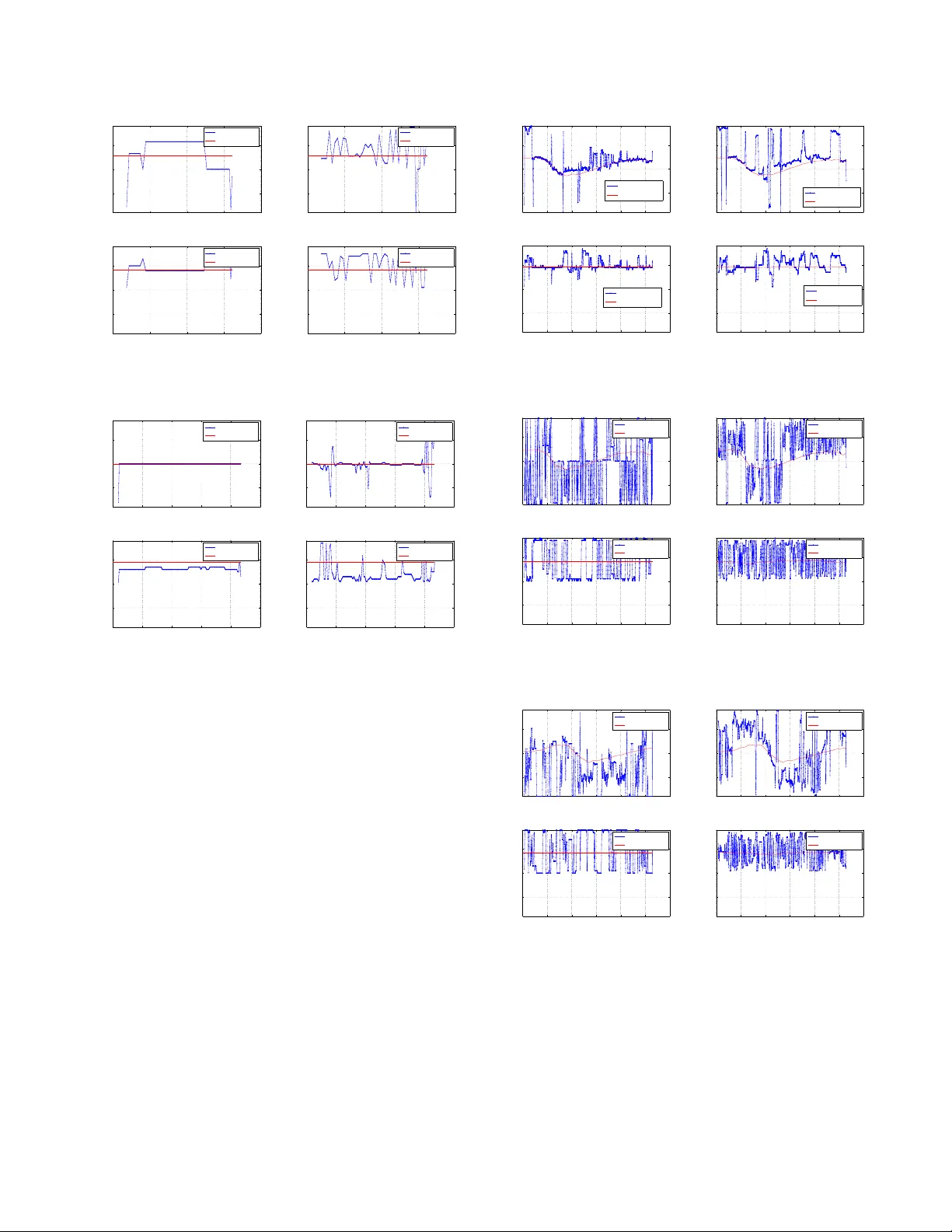
EV ALU A TING MCC-PHA T FOR THE LOCA T A CHALLENGE - T ASK 1 AND T ASK 3 Shoufeng Lin Curtin Uni versity School of Electrical Engineering, Computing and Mathematical Sciences Bentley , W estern Australia shoufeng.lin@postgrad.curtin.edu.au ABSTRA CT This report presents test results for the LOCA T A challenge [1] using the recently dev eloped MCC-PHA T (multichannel cross correlation - phase transform) sound source localization method. The specific tasks addressed are respecti v ely the localization of a single static and a single mo ving speakers using sound recordings of a variety of static microphone arrays. The test results are compared with those of the MUSIC (multiple signal classification) method. The opti- mal subpattern assignment (OSP A) metric is used for quantitati ve performance e valuation. In most cases, the MCC-PHA T method demonstrates more reliable and accurate location estimates, in com- parison with those of the MUSIC method. Index T erms — localization, MCC-PHA T , moving speaker , MUSIC, microphone array processing 1. INTRODUCTION There is a significant body of literature for the problem of sound source localization, including acoustic speaker localization in par- ticular . Obtaining accurate location estimates enables further signal processing, e.g. speaker tracking, speech separation via beamform- ing, as well as speech enhancement and dere verberation. It also has wide practical applications, e.g. automatic camera steering in smart en vironments, hearing aids and smart home assistance, as well as virtual reality synthesis. In a recent localization paper [2, 3], the author in vestigated the rev erberation-robust localization approach of using redundant in- formation of multiple microphone pairs, and proposed the Onset- MCCC and MCC-PHA T methods. The performance of the pro- posed methods has been ev aluated for static and moving speak- ers in v arious re verberant scenarios, using sound recordings from a uniform circular array (UCA). Compared with some state-of-the- art location estimators, e.g. the EB-ESPRIT [4], TF-CHB [5] and Neuro-Fuzzy [6], the proposed methods demonstrate encouraging localization capabilities. In this report, the sound corpus from LOCA T A [1] is used for ev aluating the performance of the MCC-PHA T method. Sound recordings from different microphone arrays are used. T asks of sin- gle static speaker and single moving speaker are addressed. The OSP A metric [7] was used in [3] for ev aluating localization perfor - mance in complicated scenarios, e.g. time-varying number of active speakers. In this paper , since the number of speakers is constant (only one speaker), the OSP A metric can be simplified to the root mean square (RMS). 2. PROBLEM FORMULA TION AND LOCALIZA TION ALGORITHMS 2.1. Signal Model Assuming far -field planar wa ve speaker signals, the sound recording from an arbitrary microphone i ( i = 1 , · · · , I M , I M is the total number of microphones) can be a mixture of speaker sound signals and noises. For a series of discrete time samples, x i ( n/f s ) = y q ( n/f s − τ qi ) + n i ( n/f s ) , (1a) or in the short time Fourier transform (STFT) domain X i ( ω n ) = e − ω n τ qi · Y q ( ω n ) + N i ( ω n ) , (1b) where  = √ − 1 , f s is the sampling frequenc y , n = 0 , 1 , · · · , N − 1 , N is the number of samples for the STFT , τ qi is the time delay from speaker to microphone i , ω n = 2 π f s n/ N is the angular fre- quency . y q ( n ) and Y q ( ω n ) are the speaker sound signal, and n i ( t ) and N i ( ω n ) are the additi ve noise at microphone i . For notational simplicity , the frame index is suppressed in the STFT expression. 2.2. Localization Algorithms Many algorithms rely on the signal co variance matrix, i.e. R , E [ XX H ] ≈  X ( ω n ) X H ( ω n )  , (2) where E [ · ] denotes mathematical expectation,  ·  denotes time a v- erage, the ergodicity assumption is used for the approximation, and X = [ X 1 , X 2 , · · · , X I M ] T . (3) Assuming wide sense stationarity in short time frames, and that the number of activ e sources is smaller than I M , thus the eigen- values and eigenv ectors of the covariance matrix are obtained via eigendecomposition, i.e. R V = V Λ , (4) where Λ is a diagonal matrix containing the eigen values of R in de- scending order , columns of matrix V are the corresponding eigen- vectors of R . In particular , V , [ E S | E N ] , (5) where E S is an I M × ˆ Q matrix ( ˆ Q is the estimated number of speak- ers), while E N is an I M × ˆ N matrix ( ˆ N = I M − ˆ Q ). Column vectors of the E S and E N correspond to the descending order of eigen v alues, span the signal subspace and noise subspace respec- tiv ely , and are orthonormal. 2.2.1. MUSIC The classical MUSIC method [8] formulates the localization func- tion, ε music 0 ( θ , ω n ) = 1 d H ( θ , ω n ) E N E H N d ( θ , ω n ) . (6) where θ is the direction of arri v al (DO A), and the steering vector is d ( θ , ω n ) = [ e − ω n τ 1 ( θ ) , · · · , e − ω n τ I M ( θ ) ] . (7) For wideband applications, the localization function can be e x- pressed as: ε music ( θ ) = X ω n ε music 0 ( θ , ω n ) . (8) The implementation of the MUSIC method as provided by the LO- CA T A challenge is used as the reference method. 2.2.2. MCC-PHAT [3] The standard cross-correlation function between two signals is R x i x j ( τ ) , E [ x i ( t ) x j ( t − τ )] , (9) where the goal for time delay estimation is the find the time delay τ that corresponds to the maximum cross-correlation output. The classical generalized cross-correlation (GCC) method uses the cross-power spectral density (CSD) function. Compared with the standard cross-correlation function, it improves the performance of the time delay estimation by pre-filtering signals prior to cross correlation [9, 10]. Assuming that the signal and noise power spectral density (PSD) do not vary significantly o ver frequency ranges, and the ob- servation time N /f s is much longer than the possible time delays, the CSD between observed signals is [9] S x i x j ( ω n ) ≈ N f s · E [ X i ( ω n ) · X ? j ( ω n )] . (10) The CSD between filtered outputs is G gcc ij ( ω n ) = Ψ ij ( ω n ) · S x i x j ( ω n ) , (11) where the prefilter response is Ψ ij ( ω n ) = 1 / | S x i x j ( ω n ) | for PHA T . Using the relationship between cross-correlation and CSD R x i x j ( τ ) = Z + ∞ −∞ S x i x j ( ω ) · e ωτ dω , (12) the TDO A estimation between two microphones is thus ˆ τ gcc ij = arg max τ ˜ R gcc ij ( τ ) , (13) where for discrete time signals, ˜ R gcc ij ( τ ) = N − 1 X n =0 G gcc ij ( ω n ) · e ω n τ . (14) Here ˆ τ gcc ij is the estimated time delay between the i -th and j -th mi- crophones, [ · ] ? the complex conjugate operation. The ov erall localization function of the MCC-PHA T is ε mcc − phat ( θ ) , Y ( i,j ) ∈ P j ˜ R gcc − phat ij ( τ ( θ )) k , (15) where τ is a function of θ , and the set of microphone pairs P is giv en in (16), for av oiding spatial alias. P = { ( i, j ) |k ~ m i − ~ m j k < v/f max ); i < j } , (16) where v is the velocity of sound, ~ m i is the location of microphone i , and f max is the maximum signal frequency considered. 3. NUMERICAL RESUL TS This section presents the localization results of the MCC-PHA T method using sound recordings from v arious microphone arrays, i.e. the “benchmark2”, “dicit” and “dummy”. Results using the “Eigenmike” are not provided here, as it has man y microphones, which suits particular localization algorithms and may otherwise require very long computation time for other methods. 3.1. Single Static Speaker - “T ask 1” This subsection demonstrate the performance of the MCC-PHA T method for localization of a single static speaker , which is referred to as “T ask 1” in the LOCA T A challenge. Due to av ailability of recordings, test results for the benchmark2 and dicit microphone arrays using “recording1”, while results for the dummy microphone array using “recording4” are plotted as follows. 3.1.1. Benchmark2 Fig. 1 sho ws the test results using the benchmark2 microphone ar - ray . 0 1 2 3 4 −100 0 100 Task 1, benchmark2, MccPhat Time (s) DOA ( ° ) Azimuth Ground Truth 0 1 2 3 4 −100 0 100 Task 1, benchmark2, MUSIC Time (s) DOA ( ° ) Azimuth Ground Truth 0 1 2 3 4 −100 0 100 Task 1, benchmark2, MccPhat Time (s) DOA ( ° ) Elevation Ground Truth 0 1 2 3 4 −100 0 100 Task 1, benchmark2, MUSIC Time (s) DOA ( ° ) Elevation Ground Truth Figure 1: T est results using benchmark2 microphone array . 3.1.2. DICIT Fig. 2 shows the test results using the dicit microphone array . 3.1.3. Dummy Fig. 3 shows the test results using the dummy microphone array . Fig. 1 to 3 indicate that the MCC-PHA T method seems more reliable than the MUSIC method, for the localization of a static speaker . Quantitati ve analysis is gi ven in Section 3.3. 0 1 2 3 4 −100 0 100 Task 1, benchmark2, MccPhat Time (s) DOA ( ° ) Azimuth Ground Truth 0 1 2 3 4 −100 0 100 Task 1, benchmark2, MUSIC Time (s) DOA ( ° ) Azimuth Ground Truth 0 1 2 3 4 −100 0 100 Task 1, benchmark2, MccPhat Time (s) DOA ( ° ) Elevation Ground Truth 0 1 2 3 4 −100 0 100 Task 1, benchmark2, MUSIC Time (s) DOA ( ° ) Elevation Ground Truth Figure 2: T est results using dicit microphone array . 0 2 4 6 8 10 −100 0 100 Task 1, dummy, MccPhat Time (s) DOA ( ° ) Azimuth Ground Truth 0 2 4 6 8 10 −100 0 100 Task 1, dummy, MUSIC Time (s) DOA ( ° ) Azimuth Ground Truth 0 2 4 6 8 10 −100 0 100 Task 1, dummy, MccPhat Time (s) DOA ( ° ) Elevation Ground Truth 0 2 4 6 8 10 −100 0 100 Task 1, dummy, MUSIC Time (s) DOA ( ° ) Elevation Ground Truth Figure 3: T est results using dummy microphone array . 3.2. Single Mo ving Speaker - “T ask 3” This subsection demonstrate the performance of the MCC-PHA T method for localization of a single moving speaker , which is re- ferred to as “T ask 3” in the LOCA T A challenge. T est results using “recording2” are plotted as follows. 3.2.1. Benchmark2 Fig. 4 sho ws the test results using the benchmark2 microphone ar - ray . 3.2.2. DICIT Fig. 5 shows the test results using the dicit microphone array . 3.2.3. Dummy Fig. 6 shows the test results using the dummy microphone array . From Fig. 4 to 6, both localization methods cannot work reli- ably for the moving speaker using the dicit and dummy microphone arrays. Using the benchmark2 microphone array ho we ver , can still provide locations close to ground truth. 0 5 10 15 20 25 30 −100 0 100 Task 3, benchmark2, MccPhat Time (s) DOA ( ° ) Azimuth Ground Truth 0 5 10 15 20 25 30 −100 0 100 Task 3, benchmark2, MUSIC Time (s) DOA ( ° ) Azimuth Ground Truth 0 5 10 15 20 25 30 −100 0 100 Task 3, benchmark2, MccPhat Time (s) DOA ( ° ) Elevation Ground Truth 0 5 10 15 20 25 30 −100 0 100 Task 3, benchmark2, MUSIC Time (s) DOA ( ° ) Elevation Ground Truth Figure 4: T est results using benchmark2 microphone array . 0 5 10 15 20 25 30 −100 0 100 Task 3, dicit, MccPhat Time (s) DOA ( ° ) Azimuth Ground Truth 0 5 10 15 20 25 30 −100 0 100 Task 3, dicit, MUSIC Time (s) DOA ( ° ) Azimuth Ground Truth 0 5 10 15 20 25 30 −100 0 100 Task 3, dicit, MccPhat Time (s) DOA ( ° ) Elevation Ground Truth 0 5 10 15 20 25 30 −100 0 100 Task 3, dicit, MUSIC Time (s) DOA ( ° ) Elevation Ground Truth Figure 5: T est results using dicit microphone array . 0 5 10 15 20 25 30 −100 0 100 Task 3, dummy, MccPhat Time (s) DOA ( ° ) Azimuth Ground Truth 0 5 10 15 20 25 30 −100 0 100 Task 3, dummy, MUSIC Time (s) DOA ( ° ) Azimuth Ground Truth 0 5 10 15 20 25 30 −100 0 100 Task 3, dummy, MccPhat Time (s) DOA ( ° ) Elevation Ground Truth 0 5 10 15 20 25 30 −100 0 100 Task 3, dummy, MUSIC Time (s) DOA ( ° ) Elevation Ground Truth Figure 6: T est results using dummy microphone array . 3.3. Accuracy Measur es As discussed in [3], the OSP A metric [7] is used for quantitative performance measure for localization methods, when there are car- dinality errors. When no cardinality error is tak en into consider- ation, the OSP A metric can be simplified to the root-mean square error (RMSE) metric, by choosing the power parameter to 2 . Note 0 2 4 0 2 4 6 8 10 12 14 16 18 20 Azimuth, MccPhat benchmark2 Time (s) OSPA result ( ° ) 0 2 4 0 2 4 6 8 10 12 14 16 18 20 Elevation, MccPhat benchmark2 Time (s) OSPA result ( ° ) 0 2 4 0 2 4 6 8 10 12 14 16 18 20 Azimuth, MUSIC benchmark2 Time (s) OSPA result ( ° ) 0 2 4 0 2 4 6 8 10 12 14 16 18 20 Elevation, MUSIC benchmark2 Time (s) OSPA result ( ° ) 0 2 4 0 2 4 6 8 10 12 14 16 18 20 Azimuth, MccPhat dicit Time (s) OSPA result ( ° ) 0 2 4 0 2 4 6 8 10 12 14 16 18 20 Elevation, MccPhat dicit Time (s) OSPA result ( ° ) 0 2 4 0 2 4 6 8 10 12 14 16 18 20 Azimuth, MUSIC dicit Time (s) OSPA result ( ° ) 0 2 4 0 2 4 6 8 10 12 14 16 18 20 Elevation, MUSIC dicit Time (s) OSPA result ( ° ) 0 5 10 0 2 4 6 8 10 12 14 16 18 20 Azimuth, MccPhat dummy Time (s) OSPA result ( ° ) 0 5 10 0 2 4 6 8 10 12 14 16 18 20 Elevation, MccPhat dummy Time (s) OSPA result ( ° ) 0 5 10 0 2 4 6 8 10 12 14 16 18 20 Azimuth, MUSIC dummy Time (s) OSPA result ( ° ) 0 5 10 0 2 4 6 8 10 12 14 16 18 20 Elevation, MUSIC dummy Time (s) OSPA result ( ° ) Figure 7: OSP A results for T ask1. The top row is for the MCC-PHA T method, and the bottom row is for the MUSIC method. The left three columns are for azimuth angles, while the right three columns are for elev ation angles. The RMSEs are plotted in red lines. howe v er that here the cut-off parameter is chosen as 20 ◦ for the OSP A metric. Fig. 7 and Fig. 8 provide the OSP A results for the lo- 0 10 20 30 0 10 20 Azimuth, MccPhat benchmark2 Time (s) OSPA result ( ° ) 0 10 20 30 0 10 20 Elevation, MccPhat benchmark2 Time (s) OSPA result ( ° ) 0 10 20 30 0 10 20 Azimuth, MUSIC benchmark2 Time (s) OSPA result ( ° ) 0 10 20 30 0 10 20 Elevation, MUSIC benchmark2 Time (s) OSPA result ( ° ) Figure 8: OSP A results for T ask3. The top ro w is for the MCC- PHA T method, and the bottom row is for the MUSIC method. The left column is for azimuth angles, while the right column is for ele- vation angles. The RMSE is plotted in a red line. calization methods in T ask1 and T ask3 respectiv ely . It can be seen that, except the dicit microphone for T ask1, the MCC-PHA T is in general more accurate than the MUSIC method in the test cases. 3.4. Run T ime Comparison The run times of respecti v e localization methods for T ask1 and T ask3 and used recordings are gi ven in T able 1 and T able 2. Matlab implementations of algorithms are used, and the computer hardware configuration is Intel i5-3570 3.4GHz, with 32GB RAM. T able 1: Run time (s) for T ask1 and respective recordings benchmark2 dicit dummy MUSIC 23.528503 21.401130 50.084127 MCC-PHA T 241.831558 9.719651 47.801081 T able 2: Run time (s) for T ask3 and respective recordings benchmark2 dicit dummy MUSIC 162.105479 157.904877 152.246116 MCC-PHA T 2083.525231 83.006261 168.907303 In general, the run time for respecti ve methods depends on the computing resources and time length of recordings. In particular , the required time for the MCC-PHA T method depends on the num- ber of closely placed microphone pairs, while that of the MUSIC method is more consistent (see T able 2). Howev er , it is clear that the MCC-PHA T method provides more accurate location estimates than the MUSIC method. Moreover , the localization results can be further processed with tracking filters (e.g. the GLMB filter [11] [2]) using the adaptive birth model [12], although it is beyond the scope of this paper . 4. DISCUSSIONS AND CONCLUSIONS This report presents the localization test results of the MCC-PHA T method, using sound recordings from various microphone arrays. It is interesting to note that for both tasks (T ask1 and T aks3), the benchmark2 microphone array provides most useful localization re- sults, reg ardless of the algorithms used. Besides the algorithm, the array geometry is also critical to localization performance. Comparing with the classic MUSIC method, the MCC-PHA T shows superior localization accurac y , although at the cost of higher computational load when the number of closely located micro- phones is lar ge. As shown in [2, 3], the accuracy advantage of MCC-PHA T can be more obvious in highly re v erberant en viron- ments. The rev erberation time of the LOCA T A corpus is unkno wn (it is possible that T 60 ≤ 0 . 5 ). Ho we ver , the corpus pro vides interesting test data for ev aluating location estimators for v arious scenarios. It will be e ven more useful to ha v e the re verberation time provided for respectiv e sound recordings. 5. REFERENCES [1] H. W . L ¨ ollmann, C. Evers, A. Schmidt, H. Mellmann, H. Bar - fuss, P . A. Naylor , and W . Kellermann, “The LOCA T A chal- lenge data corpus for acoustic source localization and track- ing”, IEEE Sensor Array and Multichannel Signal Processing W orkshop (SAM),(Shef field, UK) , 2018. [2] S. Lin, “JOINTL Y TRACKING AND SEP ARA TING SPEECH SOURCES USING MUL TIPLE FEA TURES AND THE GENERALIZED LABELED MUL TI-BERNOULLI FRAME- WORK”, IEEE International Confer ence on Acoustics, Speec h and Signal Pr ocessing, 2018 . ICASSP 2018. [3] S. Lin, “Re verberation-Rob ust Localization of Speakers Using Distinct Speech Onsets and Multichannel Cross Correlations”, IEEE/A CM T ransactions on A udio, Speech, and Language Pr o- cessing , vol. 26, pp.2098 - 2011, No v . 2018. [4] H. T eutsch and W . K ellermann, “ Acoustic source detection and localization based on wav efield decomposition using circular microphone arrays”, The J ournal of the Acoustical Society of America , vol. 210, no. 5, pp. 2714 - 2736, 2006. [5] A. M. T orres, M. Cobos, B. Pueo, and J. J. Lopez, “Robust acoustic source localization based on modal beamforming and timefrequency processing using circular microphone arrays”, The Journal of the Acoustical Society of America , vol. 132, no. 3, pp. 1511 -1520, 2012. [6] A. Plinge, M. H. Hennecke, and G. A. Fink, “Robust neuro- fuzzy speaker localization using a circular microphone array”, in Pr oc. Int. W orkshop on Acoustic Echo and Noise Contr ol, T el A viv , Isr ael. Citeseer , 2010. [7] D. Schuhmacher , B.-T . V o, and B.-N. V o, “ A consistent metric for performance ev aluation of multi-object filters”, IEEE T rans- actions on Signal Pr ocessing , vol. 56, no. 8, pp. 3347 - 3457, 2008. [8] R. Schmidt, “Multiple emitter location and signal parameter estimation”, IEEE transactions on antennas and pr opagation , vol. 34, no. 3, pp. 276280, 1986. [9] C. Knapp and G. Carter , “The generalized correlation method for estimation of time delay”, IEEE T r ansactions on Acous- tics, Speech, and Signal Pr ocessing , vol. 24, no. 4, pp. 320327, 1976. [10] G. C. Carter , “Coherence and time delay estimation”, Pr o- ceedings of the IEEE , vol. 75, no. 2, pp. 236255, 1987. [11] B.-N. V o, B.-T . V o, and D. Phung, “Labeled random finite sets and the bayes multi-target tracking filter”, IEEE T ransactions on Signal Pr ocessing , v ol. 62, no. 24, pp. 65546567, 2014. [12] S. Lin, B. T . V o, and S. E. Nordholm, “Measurement driv en birth model for the generalized labeled multi-bernoulli filter”, in 2016 International Confer ence on Control, A utomation and Information Sciences (ICCAIS). IEEE, 2016, pp. 9499.