A Localization Method Avoiding Flip Ambiguities for micro-UAVs with Bounded Distance Measurement Errors

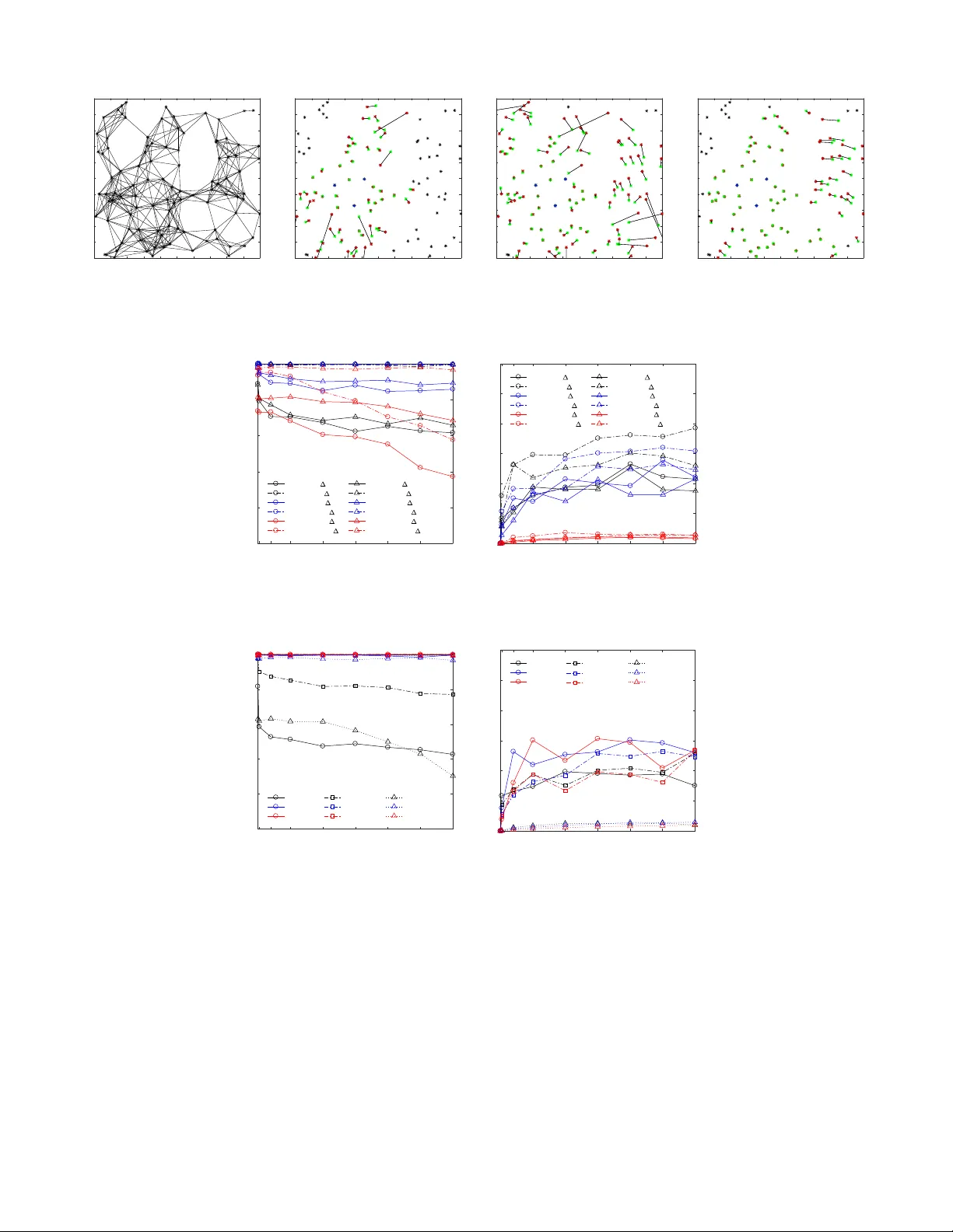
DECISION ON TMC-2017-04-0233.R2: A CCEPT AS REGULAR P APER 1 A Localization Method A v oiding Flip Ambiguities for micro-U A Vs with Bounded Distance Measurement Errors Qingbei Guo ∗ † , Y uan Zhang ∗ , Senior Member , IEEE , Jaime Lloret ‡ , Senior Member , IEEE , Burak Kantarci § , Senior Member , IEEE , W inston K.G. Seah ¶ , Senior Member , IEEE ∗ Shandong Provincial K ey Laboratory of Network based Intelligent Computing, Uni versity of Jinan, Jinan, Shandong, China Email: { ise guoqb, yzhang } @ujn.edu.cn ∗ Corresponding author † Jiangsu Provincial Engineering Laboratory of P attern Recognition and Computational Intelligence, Jiangnan Uni versity , W uxi 214122, China ‡ Integrated Management Coastal Research Institute, Uni versidad Politecnica de V alencia, Spain § School of Electrical Engineering and Computer Science, Uni versity of Otta wa, Canada ¶ School of Engineering and Computer Science V ictoria Uni versity of W ellington, New Zealand Abstract —Localization is a fundamental function in cooper - ative control of micro unmanned aerial vehicles (U A Vs), but is easily affected by flip ambiguities because of measurement errors and flying motions. This study proposes a localization method that can avoid the occurr ence of flip ambiguities in bounded distance measurement errors and constrained flying motions; to demonstrate its efficacy , the method is implemented on bilateration and trilateration. F or bilateration, an improv ed bi-boundary model based on the unit disk graph model is created to compensate f or the shortage of distance constraints, and two boundaries are estimated as the communication range constraint. The characteristic of the intersections of the communication range and distance constraints is studied to present a unique localization criterion which can a void the occurrence of flip am- biguities. Similarly , for trilateration, another unique localization criterion f or avoiding flip ambiguities is pr oposed according to the characteristic of the intersections of three distance constraints. The theoretical proof shows that these proposed criteria are correct. A localization algorithm is constructed based on these two criteria. The algorithm is validated using simulations for different scenarios and parameters, and the proposed method is shown to provide excellent localization performance in terms of av erage estimated error . Our code can be found at: https: //github .com/QingbeiGuo/AF ALA.git. Index T erms —bi-boundary model, flip ambiguity , bilateration I . I N T RO D U C T I O N T he use of multiple unmanned aerial vehicles (U A Vs) has become very popular in civil and military applications. As a key technical problem, localization of multiple mirco- U A Vs finds its application in location tracking, formation flight and cooperative mission, etc. As the most frequently used localization method, GPS suffers from large location errors of 10-30m on average. Therefore, different techniques have been proposed to address the localization problem [1]–[4]. IEEE Transactions on Mobile Computing, Submitted Apr 2, 2017 Accepted Aug 7, 2018 Localization techniques, which are based on distance measure- ment (e.g., trilateration and bilateration), hav e always attracted significant research interest [5]–[9]. Howe ver , flip ambiguity (F A) is one of the major problems of these localization techniques, especially in the presence of measurement errors [10]–[14]. The measurement error between the measurement distance and the true distance always occur because of external en vironment noise [5]–[9], that easily causes F A and results in an incorrect estimate [15] [16] [17]. Moreover , once a F A has occurred, it not only affects the current localization but also causes erroneous results for subsequent localizations. Global rigidity is widely used for localization to ensure that the result is unique [18]–[20]. A network can be uniquely located if and only if its corresponding graph is globally rigid [21]. Howe ver , ev en if the network is globally rigid in the presence of errors, F A may still occur . In trilateration, the three measured distances may locate their connected node to a false side, which causes F A due to errors in the measurements [22], [23]. Bilateration only requires network rigidity conditions to be met, not global rigidity [24]–[26], and reduces the re- liance on high node density . Ho wever , F A in bilateration deserves more attention. Giv en that only two distances exist, the localization conditions are so insufficient that additional localization constraints are required. The communication range constraint of the nodes is widely adopted as an additional localization constraint and therefore has an important role in determining the final location from the candidate locations. More importantly , an incorrect choice inevitably results in the occurrence of F A so that the estimation of the communication range of a node becomes very important. The unit disk graph [27]–[29] is commonly used to model the communication range of a wireless node. Each node has a single circle with a radius equal to a fixed value, and two nodes are connected if the distance between them is below the DECISION ON TMC-2017-04-0233.R2: A CCEPT AS REGULAR P APER 2 specified threshold. Howe ver , in reality , the boundary between reachable and unreachable areas cannot be clearly defined most of the time. Communication range between nodes is impeded by external conditions, for instance, buildings in a city [30], and internal factors, such as its energy av ailability especially after operating for long duration. Therefore, the fixed communication range assumption has its limitation in localization. Our proposed localization method is intended to address the aforementioned problems. In our method, we assume the distance measurement errors to be bounded [31] and the flying motions to be constrained [32]. An improved bi-boundary model of the communication range is proposed as localization constraints based on the model of unit disk graph. The new model depends on only distances and connectivity , and calcu- lates the double boundaries of communication ranges through the bounded measurement error . Gi ven that both bilateration and trilateration are analyzed, every constraint is regarded as a possible location region. The intersections of two distance constraints form two possible localization regions first, then the third constraint (bi-boundary and distance constraint for bilateration and trilateration, respectiv ely) is used to eliminate one region, which causes F A, by analyzing the characteristic of their intersections. Therefore, the remaining region must contain the true location and the estimated location without the possibility of F A. Accordingly , the main contributions of this paper are as follows: • An improv ed bi-boundary model based on the unit disk graph model is presented by analyzing the connectivity characteristics of a wireless node. • Based on the double constraints of distance and bi- boundary , a localization criterion that avoids F A in bi- lateration is proposed. • Another localization criterion that av oids F A in trilatera- tion is also dev eloped. • A localization algorithm based on the above two local- ization criteria, which dramatically improves the location accuracy , is constructed and ev aluated through extensi ve simulations. The rest of this paper is organized as follows: Section II introduces the related work. Section III formulates the localization problem. Section IV presents an improv ed bi- boundary model based on the unit disk graph model, describes the localization criteria that avoid F A in bilateration and trilat- eration, and provides their proofs. Based on these localization criteria, the localization algorithm is developed. In section V, the localization algorithm is validated through comprehensi ve simulation. Finally , section VI presents the conclusion. I I . R E L A T E D W O R K V arious works have in vestig ated the localization and the phenomenon of F A that may hamper the unique localization of distrib uted nodes, and have proposed different localization methods for reducing or avoiding F A. These methods can be classified into two categories: methods based on global and non-global rigidity properties which take trilateration and bilateration as representativ es, respectiv ely . Further details of these methods are provided below . A unique and anchor-free localization algorithm, which also resolves the F A problem in its second step, has been proposed by Zhang et al. [14]. A novel combination of distance and direction estimation technique is introduced to detect and estimate ranges between neighbors. Using both distance and angle information, we construct unidirectional local coordinate systems to av oid the reflection ambiguity . Howe ver , angle measurement is too expensiv e to be imbedded in most nodes, leading to few practical applications and inspiring our dev el- opment of a new localization algorithm to solve the F A issue. T rilateration is the most widely used localization method based on distance measurement [19], [21]. The estimated location of a node is determined using measured distances to three other nodes that hav e kno wn locations and are not collinear . Trilateration without measurement errors is uniquely localizable; ho wever , trilateration with measurement errors tends to suffer from the effect of F A [23], [33]. T o prev ent incorrect localization caused by F A, a robust quadrilateral was used to perform trilateration in [16], [34]– [36]. Moore et al. [16] introduced the notion of robust quadrilateral, which is a fully connected quadrilateral with global rigid properties, and used it to reduce the probability of F A. They found all possible robust quadrilaterals and then realized global localization by ov erlapping any two robust quadrilaterals that hav e three common nodes. The simulation results sho wed that the aforementioned method is suitable for the localization of high node density , because it depends on these robust quadrilaterals that require a high node density to meet the feature of global rigidity . Kannan et al. [17] pointed out that a node may be estimated at a flipped location caused by measurement errors in a globally rigid graph when its three neighboring nodes with known location are nearly collinear . They proposed a robust criterion based on the robust quadrilateral to calculate the probability of F A, to eliminate all the locations that might hav e caused it, and to improve localization performance. The simulations show that, compared with the robust quadrilateral, this method decreases not only the av erage estimation error but also the av erage number of localized nodes resulting from the rob ust criterion, which requires more constraints than the robust quadrilateral. Although more constraints can avoid problems of F A, they also limit the location of more nodes. Akcan et al. [22] proposed a heuristic solution based on the notion of a “safe-triangle” to mitigate the problem of F A in a trilateration network with range noise. First proposed here, a safe-triangle is formed by three nodes with known location, where the distance of any node to the line passing through two other nodes is larger than a set threshold. If a triangle is not a safe-triangle, its nodes are unable to provide trilateration for other nodes. The main aim is to minimize the number of F A. The simulation results show that the algorithm can achiev e better performance than trilateration. Howe ver , similar to trilateration, the safe-triangle algorithm also requires a high node density . T o reduce localization dependence on global rigidity , many algorithms [24], [25], [27] are proposed for network local- DECISION ON TMC-2017-04-0233.R2: A CCEPT AS REGULAR P APER 3 ization using bilateration which requires rigid conditions but not necessarily globally rigid. Based on [24], Goldenberg et al. [25] proposed the “Sweeps” algorithm for network localization using bilateration. The Sweeps algorithm achiev es one of the best performance in terms of number of localized nodes using bilateration. Howe ver , the algorithm requires a bilateration ordering to exist in the network, a condition which does not always exist in a sparse network; thus, it may fail in many localizable networks [25], [26]. Oliv a et al. [27] introduced a model of shadow edges to extend trilateration to bilateration, which can produce effecti ve solutions despite the lack of localization condition. The algo- rithm shows better performance than trilateration, and is able to localize the network even when trilateration fails. Howe ver , this method is based on unit disk graphs and only limited to noiseless environments. The objectiv e of our research is to av oid the occurrence of F A and achiev e the accurate localization network using trilateration and bilateration with the errors including bounded measurement errors and constrained motions. A localization algorithm is proposed based on two classes of localization criteria that av oid the F A problem. In our algorithm, the two classes of localization criteria are deriv ed by gradually analyz- ing the intersection characteristic of all the constrains. Then, trilateration and bilateration are combined to take adv antage of the best of them, thus making them applicable in various kinds of networks that are sparse or not. I I I . P RO B L E M F O R M U L AT I O N W ithout loss of generality , the localization problem of a micro-U A V network modelled as a mobile sensor network can be formulated in 2D space [37], [38]. Multiple micro- U A Vs, which consists of a set of n nodes, denoted as s 1 to s n , are flying in a physical region. Each node has a limited communication range and establishes a wireless link with a neighboring node, which is called its neighboring node only if they are within the communication range of each other . A node is assumed to be capable of estimating the distance to the neighboring node using distance measurement technology . Gi ven the constraints on energy consumption and implementation environment, most nodes do not know their locations except anchors which can obtain their own locations by using GPS. In this study , the micro-U A V network is analyzed without anchor nodes. The communication range of node s i is denoted by r i , and its estimated communication range by ˆ r i , its true location by p i , and its estimated location by ˆ p i . The true distance between any two neighboring nodes s i and s j is denoted by d ij , and the measured distance by ˆ d ij , where i , j = 1,2,. . . , n . For a connected network, we assume that the distances between neighboring nodes can be acquired in a time unit [39]. The speed of a node s i is the distance trav elled by the node per time unit [32], denoted as d i , and d max is the maximum distances travelled by these nodes in a time unit. Therefore, in each time unit, the micro-UA V network can be described by a model of undirected graph G t = ( V , E ) with a nonempty vertex set V = { 1,2,. . . , n } and edge set E , where each vertex i ∈ V uniquely represents a node s i , and each edge e ( i, j ) ∈ E is uniquely associated with a node pair ( s i , s j ), for which s i and s j are neighbors, and ˆ d ij is known. The measurement error of e ( i, j ) is denoted by e ij such that e ij = d ij − ˆ d ij , and e max is the maximum measurement errors. The network topology can and will change in the different time units because of the measurement errors and the flying trajectories. Howe ver , during the localization process, s i has a possible localization region set R i = { r i 1 , r i 2 } and corresponding candidate location set P i = { p i 1 , p i 2 } because of the F A phenomenon. While the true location p i is dif ficult to be determined due to the errors consisting of the measurement errors and the flying distances, R i and P i can be determined by the measured distances and the errors. F A occurs when the estimated location and the true location are not in the same lo- calization region. Therefore, to determine the true localization region becomes a key problem in deciding whether F A occurs. By gradually analyzing the characteristic of the intersections corresponding to all the constraints, our method eliminates the localization region in which each location causes F A instead of choosing which one contains the true location. Therefore, the remaining region is identified as the true localization region, and the corresponding candidate location is regarded as the estimated location with no possibility of F A. I V . L O C A L I Z AT I O N C R I T E R I A A N D L O C A L I Z A T I O N A L G O R I T H M A. Bi-boundary Model of Communication Range Constraint In this section, an impro ved bi-boundary model based on the unit disk graph is presented to model the topology of wireless sensor networks with the errors which consist of the bounded measurement errors and the constrained motions. Now , we first focus on the ef fect of only the measurement errors, and the flying motions will be introduced in Section IV.D. In this bi-boundary model, each node has double concentric circles with two different radii, and the space between two circles represents an uncertainty in the communication range. The inner and outer boundaries represent the lower limit of the reachable range and the upper limit of the unreachable range, respecti v ely; thus, this bi-boundary design is more suitable for the actual en vironment. The calculation of the two boundaries is independent of the measuring technique and instead completely depends on the kno wledge of the distances, the measurement errors and connectivity between nodes, without maintaining the individual parameter of the communication range. The process of estimating the upper and lower boundaries of a wireless node is giv en in detail below . Let ε > 0 be a threshold of the distance variation, such that | e ij | = | d ij − ˆ d ij | ≤ ε = e max . Thus, d ij ∈ [ ˆ d ij − ε, ˆ d ij + ε ] . (1) Follo wing the aforementioned analysis on the neighboring node and communication noise, for ev ery node s i , the esti- mated communication range ˆ r i can be bounded as ˆ r i ≥ max ( D 1 i ) − ε, (2) DECISION ON TMC-2017-04-0233.R2: A CCEPT AS REGULAR P APER 4 s p s o s q s i ε 2 ε Fig. 1. Example of estimating the communication range. For node s i , the minimum of the estimated communication range is ˆ d io − ε , and the maximum is ˆ d pi + ˆ d pq + 2 ε . where D k i represents the measured distance set between the nodes that are at least k -hop aw ay from node s i , where k = 1,2,. . . , n . In particular, D 1 i = { ˆ d ij | e ( i, j ) ∈ E } , D 2 i = { ˆ d il + ˆ d lj | e ( i, j ) / ∈ E , e ( i, j ) ∈ E , e ( i, j ) ∈ E , and l 6 = i , l 6 = j } . T o further analyze r i , the scenario is illustrated in Fig. 1. Giv en the unknown location of s i which is connected with both s o and s p but is not connected with s q , ˆ d iq cannot be directly calculated using p i and p q ; thus, it cannot contribute to the estimation of r i . The sum of any two sides of a triangle is greater than the third side, so that r i is less than the sum of any 2 -hop distance from s i to s q . Therefore, considering the factor of the measurement errors, the following condition must be satisfied: ˆ r i < min ( D 2 i ) + 2 ε. (3) Finally , the estimated communication range ˆ r i , which satisfies equations (2) and (3), is bounded as follo ws: max ( D 1 i ) − ε ≤ ˆ r i < min ( D 2 i ) + 2 ε. (4) The connection property of a node therefore affects its esti- mated result. Moreover , higher node density , which increases the degree of node connectivity , makes the estimate more precise. B. F A A voidance Criteria for Localization using Bilateration In this section, we introduce the scenario of using bilatera- tion and present a localization criteria for av oiding F A using the bi-boundary and distance constraints. Fig. 2 represents the corresponding graph of localization without flip ambiguities using bilateration. Fig. 2 (a) shows a normal case without near-collinear and ov erlapping occurrences. Fig. 2 (b) and (c) depict a near -collinear case and an o verlapping case, respectiv ely . Moreover , a compositive case with near-collinear and overlapping occurrences is shown in Fig. 2 (d). For each case above, we will follow the same process because our proposed localization method adapts to all the cases. The location of node s o is assumed to be the origin, and another node s p is selected to form the positive x -axis, and the third node s q is located in the upper half-plane. The intersections of the black annulus and the red annuli form the upper re gion r q 1 , which is the possible localization region of s q . The possible localization regions of s i are the two regions r i 1 and r i 2 consisting of the intersections of the gray annulus and the blue annuli. The three regions of r r 1 , r r 2 and r q 1 are highlighted with horizontal stripes, vertical stripes and mesh, respectiv ely . u and v are any points of r q 1 and r i 1 , respecti vely , and their communication ranges are denoted by the green annulus and the yellow annulus, respectiv ely . Obviously , both u and v are within the communication range of each other , and hence they must be adjacent. Furthermore, each point of r i 1 clearly is within the communication range of u ; thus, for u , the whole region r i 1 is not a possible localization region of s i . Note that due to the uncertainty of the true location p p , there exist countless red annuli and blue annuli whose centers are at every point in between ( ˆ d op − ε, 0) and ( ˆ d op + ε, 0) , but only two red annuli and two blue annuli at both ends are shown to simplify the figure. The true distances d op , d oq and d pq among the three nodes can be bounded as follows: d op ∈ [ ˆ d op − ε, ˆ d op + ε ] , (5) d oq ∈ [ ˆ d oq − ε, ˆ d oq + ε ] , (6) d pq ∈ [ ˆ d pq − ε, ˆ d pq + ε ] . (7) It is obvious that the true location p p of s p is between ( ˆ d op − ε, 0) and ( ˆ d op + ε, 0) . The true location p q of node s q is calculated based on p o , p p , d oq and d pq . Based on equations (6) and (7), the two close intervals form two annulus regions, which can be defined using ˆ d oq and ˆ d pq as r oq = { ( x, y ) | ( ˆ d oq − ε ) 2 ≤ ( x − x o ) 2 + ( y − y o ) 2 ≤ ( ˆ d oq + ε ) 2 } , (8) r pq = { ( x, y ) | ( ˆ d pq − ε ) 2 ≤ ( x − x p ) 2 + ( y − y p ) 2 ≤ ( ˆ d pq + ε ) 2 } , (9) where ( x o , y o ) and ( x p , y p ) are the location coordinates of s o and s p , respectiv ely . Since s o is assumed to be the origin, equation (8) can be also written as follo ws: r oq = { ( x, y ) | ( ˆ d oq − ε ) 2 ≤ x 2 + y 2 ≤ ( ˆ d oq + ε ) 2 } . (10) Howe ver , as equation (5) sho ws, the true location p p is uncertain. Thus, equation (9) can be also written as follows: r pq = { ( x, y ) | (( ˆ d pq − ε ) 2 ≤ ( x − ˆ d op + ε ) 2 + y 2 ≤ ( ˆ d pq + ε ) 2 ) ∨ (( ˆ d pq − ε ) 2 ≤ ( x − ˆ d op − ε ) 2 + y 2 ≤ ( ˆ d pq + ε ) 2 ) } . (11) The intersections of r oq and r pq form the two regions r q 1 and r q 2 . The two regions are certainly symmetrical with respect to the edge e ( o, p ) , but they can be adjacent or nonadjacent in various situations [17]. T o ensure that they are separated, the edge e ( o, p ) is added as the boundary between them. The half- plane that contains s q is denoted by H , and the complementary half-plane is denoted by H 0 . Hence, H and H 0 can be written as follows: H = { ( x, y ) | y > 0 } , (12) DECISION ON TMC-2017-04-0233.R2: A CCEPT AS REGULAR P APER 5 s o s p r q 1 r i 2 r i 1 u v d uv s q s i 2 s i 1 (a) Noraml case s o s p r q 1 r i 2 r i 1 u v d uv s q s i 2 s i 1 (b) Near-collinear case s o s p r q 1 r i 2 r i 1 u d uv s q s i 1 s i 2 v (c) Overlapping case s o s p r q 1 r i 2 r i 1 u d uv s q s i 2 s i 1 v (d) Both near-collinear case and over- lapping case Fig. 2. Localization without flip ambiguities using bilateration. H 0 = { ( x, y ) | y ≤ 0 } . (13) Thus, the possible localization re gion of node s q can be defined as follows: r q 1 = { ( x, y ) | ( x, y ) ∈ r oq ∩ r pq ∩ H } . (14) Similarly , this method can also be extended to the analysis of the possible localization regions of s i . The two annulus regions related with s i can be defined as follows: r oi = { ( x, y ) | ( ˆ d oi − ε ) 2 ≤ x 2 + y 2 ≤ ( ˆ d oi + ε ) 2 } , (15) r pi = { ( x, y ) | (( ˆ d pi − ε ) 2 ≤ ( x − ˆ d op + ε ) 2 + y 2 ≤ ( ˆ d pi + ε ) 2 ) ∨ (( ˆ d pi − ε ) 2 ≤ ( x − ˆ d op − ε ) 2 + y 2 ≤ ( ˆ d pi + ε ) 2 ) } . (16) Thus, the two possible localization regions of s i can be defined as follows: r i 1 = { ( x, y ) | ( x, y ) ∈ r oi ∩ r pi ∩ H } , (17) r i 2 = { ( x, y ) | ( x, y ) ∈ r oi ∩ r pi ∩ H 0 } . (18) The true location of node s i is in one of the two regions r i 1 or r i 2 . T o obtain an unambiguous estimated location, additional knowledge is required to determine which region contains the true location. In this paper, the communication ranges of the nodes s q and s i are used to address the ambiguity problem. According to the aforementioned bi-boundary model, the communication ranges of s q and s i can be bounded as follows: r q ∈ [ max ( D 1 q ) − ε, min ( D 2 q ) + 2 ε ] , (19) r i ∈ [ max ( D 1 i ) − ε, min ( D 2 i ) + 2 ε ] . (20) Hence, the maximum communication distance, within which s q and s i can certainly communicate with each other, is defined by: D q i = min ( max ( D 1 q ) − ε, max ( D 1 i ) − ε ) . (21) Lastly , Theorem 1 prov es whether node s i can be uniquely localizable in 4 opq . Theorem 1. Given a localized triangle 4 opq , wher e its three localized nodes s o , s p and s q ar e adjacent to each other , and an unknown node s i , such that the edges e ( o, i ) and e ( p, i ) exist, but e ( q , i ) does not exist. Let ε = e max > 0 be a thr eshold of the distance measurement err ors. s i can be a unique localization, and its suf ficient conditions ar e as follows: (1) ∀ x ∈ r q 1 , ∀ y ∈ r i 1 , d xy < D q i , (2) ∃ u ∈ r q 1 , ∃ v ∈ r i 2 , d uv > D q i . Pr oof. r i 1 and r i 2 are two possible localization regions of s i based on constraints of the two distance ˆ d oi and ˆ d pi . If every pair of points between r q 1 and r i 1 are adjacent while at least one pair of points between r q 1 and r i 2 are beyond D q i , then the whole region r i 1 is excluded as a possible localization region of s i . Therefore, the region r i 2 is the only possible region which contains the true location p i , and no possibility exists for the occurrence of F A. In this case, both nodes s i and s q are clearly on the opposite of the edge e ( o, p ) . C. F A A voidance Criteria for Localization using T rilateration W e now address the scenario where trilateration is used without flip ambiguities, and Fig. 3 shows the corresponding graph of this scenario. Just like Fig. 2, a normal case is depicted without near-collinear and overlapping occurrences in Fig. 3 (a). Fig. 3 (b) and (c) show a near-collinear case and an overlapping case, respectiv ely . And then, Fig. 3 (d) shows a compositiv e case with near-collinear and ov erlapping occur- rences. Due to the feasibility of our method to all the cases, we will also follow the same process. The detection of the F A occurrences is now analyzed. The possible localization region of s q is the upper region r q 1 consisting of the intersections of the black annulus and the red annuli. The intersections of the gray annulus and the blue annuli form two regions r i 1 and r i 2 , which are the possible localization regions of s i . The three regions highlighted with horizontal stripes, vertical stripes and mesh indicate r r 1 , r r 2 and r q 1 , respecti vely . u and v are any points of r q 1 and r i 1 , respecti vely . Since d uv / ∈ [ ˆ d q i − ε, ˆ d q i + ε ] , v is without the constraints of the distance ˆ d q i , and each point of r i 1 is clearly without the constraint of ˆ d q i . Therefore, for u , the whole region r i 1 is not a possible localization region of s i . DECISION ON TMC-2017-04-0233.R2: A CCEPT AS REGULAR P APER 6 s o s p r q 1 r i 2 r i 1 u v d uv s q s i 2 s i 1 (a) Noraml case s o s p r q 1 r i 2 r i 1 u v d uv s q s i 2 s i 1 (b) Near-collinear case s o s p r q 1 r i 2 u d uv s q s i 1 s i 2 v r i 1 (c) Overlapping case s o s p r q 1 u d uv s i 2 v s q r i 2 r i 1 s i 1 (d) Both near-collinear case and over- lapping case Fig. 3. Localization without flip ambiguities using trilateration. Similar to the analysis for the scenario using bilateration, the two annuli r oq and r pq are also respectiv ely defined as follows: r oq = { ( x, y ) | ( ˆ d oq − ε ) 2 ≤ x 2 + y 2 ≤ ( ˆ d oq + ε ) 2 } , (22) r pq = { ( x, y ) | (( ˆ d pq − ε ) 2 ≤ ( x − ˆ d op + ε ) 2 + y 2 ≤ ( ˆ d pq + ε ) 2 ) ∨ (( ˆ d pq − ε ) 2 ≤ ( x − ˆ d op − ε ) 2 + y 2 ≤ ( ˆ d pq + ε ) 2 ) } . (23) Thus, the possible localization region of node s q is also defined as follows: r q 1 = { ( x, y ) | ( x, y ) ∈ r oq ∩ r pq ∩ H } . (24) Similarly , using the two measured distances ˆ d oi and ˆ d pi that are affected by noises, the two annuli r oi and r pi are also respectiv ely defined as follo ws: r oi = { ( x, y ) | ( ˆ d oi − ε ) 2 ≤ x 2 + y 2 ≤ ( ˆ d oi + ε ) 2 } , (25) r pi = { ( x, y ) | (( ˆ d pi − ε ) 2 ≤ ( x − ˆ d op + ε ) 2 + y 2 ≤ ( ˆ d pi + ε ) 2 ) ∨ (( ˆ d pi − ε ) 2 ≤ ( x − ˆ d op − ε ) 2 + y 2 ≤ ( ˆ d pi + ε ) 2 ) } . (26) Follo wing which, the two possible localization regions of s i are also defined as follows: r i 1 = { ( x, y ) | ( x, y ) ∈ r oi ∩ r pi ∩ H } , (27) r i 2 = { ( x, y ) | ( x, y ) ∈ r oi ∩ r pi ∩ H 0 } . (28) The true location p i must be located in one of the two separated regions r i 1 and r i 2 , but incorrect calculation can cause F A; thus, to address the problem of F A and deriv e the estimated location, we use a third annulus r q i , which is defined by the following equation: r q i = { ( x, y ) | ( ˆ d q i − ε ) 2 ≤ ( x − x q ) 2 + ( y − y q ) 2 ≤ ( ˆ d q i + ε ) 2 } . (29) T o summarize, we have the follo wing theorem: Theorem 2. Given a localized triangle 4 opq , wher e its three localized nodes s o , s p and s q ar e adjacent to each other , and an unknown node s i , such that the edges e ( o, i ) , e ( p, i ) and e ( q , i ) exist. Let ε = e max > 0 be a threshold of the distance measur ement err ors. s i can be a unique localization, and its sufficient conditions are as follows: (1) ∀ x ∈ r q 1 , ∀ y ∈ r i 1 , d xy / ∈ [ ˆ d q i − ε, ˆ d q i + ε ] , (2) ∃ u ∈ r q 1 , ∃ v ∈ r i 2 , d uv ∈ [ ˆ d q i − ε, ˆ d q i + ε ] . Or , (1) ∀ x ∈ r q 1 , ∀ y ∈ r i 2 , d xy / ∈ [ ˆ d q i − ε, ˆ d q i + ε ] , (2) ∃ u ∈ r q 1 , ∃ v ∈ r i 1 , d uv ∈ [ ˆ d q i − ε, ˆ d q i + ε ] . Pr oof. Follo wing the same analysis in Theorem 1, r i 1 and r i 2 are two possible localization regions of s i based on constraints of the two distances ˆ d oi and ˆ d pi . There are at least one pair of points, whose distances are under the constraints of the third distance ˆ d q i , between r q 1 and r i 2 (or r i 1 ), whereas there is no any pair of points, whose distance is without the constraints of the third distance ˆ d q i , between r q 1 and r i 1 (or r i 2 ). Thus, the whole region r i 1 (or r i 2 ) is eliminated from the possible localization regions of s i , and the other region r i 2 (or r i 1 ) is a unique estimated region that causes no F A. D. Localization Considering V elocities and Dir ections Considering the motion velocities and directions of micro- U A Vs, we further introduce our localization criteria av oiding F A in trilateration and bilateration. For a connected network, we first assume that the location update can be completed in one time unit. Since the velocities and directions vary , they are represented as the motion distances per time unit [32]. The size and sign of the motion distances are used to denote the magnitude and direction of motions. Here, positive v alue indicates that a node moves in the opposite direction, leading to an increase of distances between nodes, while negati ve v alue indicates the motion tow ards each other . When the distances between neighboring nodes are acquired together in a time unit, the possible locations of each node fall into a larger region due to their motions. Combining the factor of measurement errors mentioned abov e, the distance d ij between any two neighboring nodes s i and s j can be re-constrained as follows: d ij ∈ [ ˆ d ij − ( e max + d max ) , ˆ d ij + ( e max + d max )] . (30) DECISION ON TMC-2017-04-0233.R2: A CCEPT AS REGULAR P APER 7 0 10 20 30 40 50 60 70 80 90 100 0 10 20 30 40 50 60 70 80 90 100 (a) A random network graph 0 10 20 30 40 50 60 70 80 90 100 0 10 20 30 40 50 60 70 80 90 100 (b) TLA 0 10 20 30 40 50 60 70 80 90 100 0 10 20 30 40 50 60 70 80 90 100 (c) SELA 0 10 20 30 40 50 60 70 80 90 100 0 10 20 30 40 50 60 70 80 90 100 (d) AF ALA Fig. 4. Comparison of TLA, SELA and AF ALA on a random graph with r =20, δ =0.02 and ε = δ , where green and red tic marks denote the true and estimated locations, respectively . 0 0.02 0.2 0.5 1 1.5 2 2.5 3 measurement error 0 20 40 60 80 100 percentage of localized nodes TLA n=50 r TLA n=100 r SELA n=50 r SELA n=100 r AFALA n=50 r AFALA n=100 r TLA n=50 s TLA n=100 s SELA n=50 s SELA n=100 s AFALA n=50 s AFALA n=100 s (a) %localized nodes 0 0.02 0.2 0.5 1 1.5 2 2.5 3 measurement error 0 20 40 60 80 100 120 average estimated error TLA n=50 r TLA n=100 r SELA n=50 r SELA n=100 r AFALA n=50 r AFALA n=100 r TLA n=50 s TLA n=100 s SELA n=50 s SELA n=100 s AFALA n=50 s AFALA n=100 s (b) A verage estimation error Fig. 5. Impact of initial triangle. r = 30, d max = 0. r 4 and s 4 denote the random and special triangle, respectiv ely . 0 0.02 0.2 0.5 1 1.5 2 2.5 3 measurement error 0 20 40 60 80 100 percentage of localized nodes TLA r=20 TLA r=30 TLA r=40 SELA r=20 SELA r=30 SELA r=40 AFALA r=20 AFALA r=30 AFALA r=40 (a) %localized nodes 0 0.02 0.2 0.5 1 1.5 2 2.5 3 measurement error 0 20 40 60 80 100 120 average estimated error TLA r=20 TLA r=30 TLA r=40 SELA r=20 SELA r=30 SELA r=40 AFALA r=20 AFALA r=30 AFALA r=40 (b) A verage estimation error Fig. 6. Impact of measurement error. n = 100, s 4 , d max = 0. These two parameters, measurement error and motion, are regarded as the influential factors on distance-based local- izations. Therefore, the dynamic localization problem can be formulated with ε = e max + d max . According to theorem 1 and 2, two lemmas in trilateration and bilateration can be induced. Lemma 1. Given a localized triangle 4 opq , wher e its thr ee localized nodes s o , s p and s q ar e adjacent to each other , and an unknown node s i , such that the edges e ( o, i ) and e ( p, i ) exist, but e ( q , i ) does not e xist. Let ε = e max + d max > 0 be a thr eshold of the distance variations. s i can be a unique localization, and its sufficient conditions ar e as follows: (1) ∀ x ∈ r q 1 , ∀ y ∈ r i 1 , d xy < D q i , (2) ∃ u ∈ r q 1 , ∃ v ∈ r i 2 , d uv > D q i . Lemma 2. Given a localized triangle 4 opq , wher e its thr ee localized nodes s o , s p and s q ar e adjacent to each other , and an unknown node s i , such that the edges e ( o, i ) , e ( p, i ) and e ( q , i ) exist. Let ε = e max + d max > 0 be a threshold of the distance variations. s i can be a unique localization, and its sufficient conditions are as follows: (1) ∀ x ∈ r q 1 , ∀ y ∈ r i 1 , d xy / ∈ [ ˆ d q i − ε, ˆ d q i + ε ] , (2) ∃ u ∈ r q 1 , ∃ v ∈ r i 2 , d uv ∈ [ ˆ d q i − ε, ˆ d q i + ε ] . DECISION ON TMC-2017-04-0233.R2: A CCEPT AS REGULAR P APER 8 50 100 150 200 network density 75 80 85 90 95 100 percentage of localized nodes (a) %localized nodes 50 100 150 200 network density 0 20 40 60 80 average estimated error (b) A verage estimation error Fig. 7. Impact of network density . s 4 , r = 30, d max = 0. 0 0.2 0.4 0.6 0.8 1 1.2 1.4 1.6 1.8 2 speed 75 80 85 90 95 100 percentage of localized nodes (a) %localized nodes 0 0.2 0.4 0.6 0.8 1 1.2 1.4 1.6 1.8 2 speed 0 20 40 60 80 100 average estimated error (b) A verage estimation error Fig. 8. Impact of node motion. n = 150, s 4 , r = 20. Or , (1) ∀ x ∈ r q 1 , ∀ y ∈ r i 2 , d xy / ∈ [ ˆ d q i − ε, ˆ d q i + ε ] , (2) ∃ u ∈ r q 1 , ∃ v ∈ r i 1 , d uv ∈ [ ˆ d q i − ε, ˆ d q i + ε ] . E. Localization Algorithm Based on the aforementioned criteria, we now present our A voiding Flip Ambiguities Localization Algorithm (AF ALA). The algorithm first selects a random triangle or a special triangle, which is an acute triangle with ev ery edge greater than four fifths of the communication ranges, as the initial triangle and adds its three nodes to a set of localized nodes. For any unlocalized node, if it is connected to these three localized nodes and the condition of Theorem 1 or Lemma 1 is satisfied, or it is connected to two localized nodes and the condition of Theorem 2 or Lemma 2 is satisfied, it is localized and is mov ed from the unlocalized nodes set to the localized nodes set. The process is iterated until no new node can join the set of localized nodes. Details are sho wn in Algorithm 1. V . P E R F O R M A N C E V A L I D A T I O N In this section, the localization performance of the proposed algorithm is compared with TLA [21] and SELA [27] in terms of the percentage of localizable nodes and the average estimation error , using simulations implemented in MA TLAB 7.14.0.739 (R2012a). Simulations are conducted in a square unit area of 100 units by 100 units , where micro-U A Vs are uniformly distributed. 100 random instances of micro-U A V network are administered in each group trial, and the av erage result is tak en to ensure more accurate result. The e xperimental parameter settings are as follows: • The number n of micro-U A Vs deployed in networks ranges from 50 to 200; • A random or special triangle is randomly chosen as the initial triangle; • The communication radius r is set to be 20, 30 and 40 units ; • The measurement errors e ij ∼ N (0 , δ 2 ) , such that ˆ d ij = | d ij + e ij | , where δ is set to be 0, 0.02, 0.2, 0.5, 1, 1.5, 2, 2.5 and 3 units ; • The motion speed of each micro-U A V is randomly chosen from [ − d max , d max ] units per time unit, where the maximum motion speed d max is set to be 0:0.2:2 units per time unit; • The motion factor is considered or not by the threshold value ε which is set to be δ or δ + d max . In order to keep the errors within the maximum allowable bounds, if | d ij − ˆ d ij | > ε , then | d ij − ˆ d ij | = ε . Fig. 4 presents a representative localization scenario with r = 20 and δ = 0.2. Fig. 4 (a) shows the original graph of the network. Fig. 4 (b), (c) and (d) present the localization results of the TLA, SELA and AF ALA algorithms in the same scenario. The three blue nodes are randomly chosen as the nodes of the initial triangle. The green and red nodes are the DECISION ON TMC-2017-04-0233.R2: A CCEPT AS REGULAR P APER 9 Algorithm 1 the AF ALA algorithm based on both localization criteria. Require: A set of unlocalized nodes, S u ; A set of localized triangles, S t ; The threshold value of distance variations, ε ; Ensure: A set of localized nodes, S l ; 1: choose an initial triangle 4 opq into S t ; 2: add the three nodes of 4 opq to S l ; 3: repeat 4: for each node s i ∈ S u do 5: for each localized triangle 4 opq ∈ S t do 6: if s i connects to two nodes s o and s p then 7: r q 1 = r oq ∩ r pq ∩ H ; 8: r i 1 = r oi ∩ r pi ∩ H ; 9: r i 2 = r oi ∩ r pi ∩ H 0 ; 10: [ G q 1 , G i 1 , G i 2 ] = the set of grid point coordinate of r q 1 , r i 1 and r i 2 , respectively; 11: if s i connects to the node s q then 12: if (( ∀ x ∈ G q 1 , ∀ y ∈ G i 1 , d xy < ˆ d q i − ε ∧ d xy > ˆ d q i + ε ) AND ( ∃ u ∈ G q 1 , ∃ v ∈ G i 2 , ˆ d q i − ε < d uv < ˆ d q i + ε )) OR (( ∃ x ∈ G q 1 , ∃ y ∈ G i 1 , ˆ d q i − ε < d xy < ˆ d q i + ε ) AND ( ∀ u ∈ G q 1 , ∀ v ∈ G i 2 , d uv < ˆ d q i − ε ∧ d uv > ˆ d q i + ε )) then 13: calculate the estimated location ˆ p i ; 14: mov e s i from S u to S l ; 15: update the distances of the localized sub- graph 16: add 4 opi to S t ; 17: end if 18: else 19: D q i = min ( max ( D 1 q ) − ε, max ( D 1 i ) − ε ) ; 20: if ( ∀ x ∈ G q 1 , ∀ y ∈ G i 1 , d xy < D q i ) AND ( ∃ u ∈ G q 1 , ∃ v ∈ G i 2 , d uv > D q i ) then 21: calculate the estimated location ˆ p i ; 22: mov e s i from S u to S l ; 23: update the distances of the localized sub- graph 24: add 4 opi to S t ; 25: end if 26: end if 27: end if 28: end for 29: end for 30: until the element number of S l no longer changes 31: retur n S l ; true and estimated locations, respectiv ely , which are connected with black lines, while the remaining black parts are the unlocated nodes. Ob viously , the SELA and AF ALA algorithms locate more nodes than TLA because of the utilization of bilateration. Howe ver , many F As occur in the TLA and SELA algorithms, while no F As occur in AF ALA. That is because our algorithm, AF ALA, fully consider the effect of measurement error on F A. Therefore, our algorithm locates more accurately than TLA and SELA. W e further demonstrate the localization performance in terms of percentage of localized nodes and average estimation error by comparing AF ALA with TLA and SELA from aspects such as initial triangle, measurement error , network density and node motion. A. Initial T riangle: Random & Special T riangle As the starting point of algorithms, the choice of initial triangles determines whether algorithms can localize their first new node. If the node fails to be localized, that means the localization process was ov er before initiating. Fig. 5 shows the effect of random and special triangle on the localization performance. As is shown in Fig. 5 (a), for ev ery network density , these three algorithms (especially AF ALA) with spe- cial triangle distinctly localizes more nodes than with random triangle under the same measurement errors. Furthermore, with the increase of measurement errors, the number of nodes localized by AF ALA algorithm with random triangle rapidly drops. In contrast, the special triangle slowly decreases the number of localized nodes. Especially , when network density is equal to 100, the number of localized nodes with special triangle almost remains stable, even reaching to about 100%. Theoretically , the special triangle more easily satisfies the localization criteria of AF ALA, thus improving the number of localized nodes. Fig. 5 (b) shows the effect of random and special triangle on the av erage estimation error . Obviously , the initial triangle tends to have less impact on AF ALA than both TLA and SELA. Therefore, the choice of the initial triangle significantly affects the localization result of these methods, and special triangle achie ves better localization performance than random triangle in terms of the localization ratio. B. Measur ement Err or W e demonstrate the impact of measurement errors on the localization performance in terms of percentage of localized nodes and av erage estimation error in Fig. 6. Fig. 6 (a) shows the percentage of localized nodes against the measurement er- ror . For r = 20, the AF ALA and SELA algorithms locate more nodes than TLA when the measurement error is small, espe- cially SELA. Ho we ver , as the measurement error increases, the percentage of localized nodes decreases markedly in AF ALA. That is mainly because the strict localization conditions of AF ALA are difficult to satisfy with small communication radius and large measurement errors. For the large communi- cation radius r = 30 and 40, the performance gap among the three algorithms decreases gradually . Especially for r = 40, they are able to localize almost all the nodes. That is because DECISION ON TMC-2017-04-0233.R2: A CCEPT AS REGULAR P APER 10 the large communication radius increases the possibility of using trilateration and reduces the key differences among these algorithms. For the case of AF ALA, the localization conditions are also easily satisfied, leading to good outcomes. Fig. 6 (b) sho ws the a verage estimation error against the measurement error where AF ALA performs significantly better than TLA and SELA. For ev ery value of r , it is apparent that the av erage estimation error is much less in AF ALA than in TLA and SELA. Thus, the proposed algorithm exhibits excellent localization performance in terms of the average estimation error . This confirms the efficac y of AF ALA as it addresses the critical issue of measurement errors, a k ey source of F A, to fulfil the criteria for accurate localization. C. Network Density Fig. 7 illustrates the impact of network density on the localization performance in different localization algorithms. Fig. 7 (a) sho ws the impact of network density on the localization ratio. For TLA, SELA and AF ALA, the number of localized nodes significantly increases with the increase of network density . SELA achieves the fastest growth due to its most flexible localization conditions. On the contrary , AF ALA obtains the lowest gro wth because of its most rigorous conditions. Ho wev er , the gap among them is gradually reduced with the increase of network density . When network density is larger than 120, AF ALA localizes almost all the nodes, reaching nearly the same localization ratio of TLA and SELA. Fig. 7 (b) shows the impact of network density on the av erage estimation error . Although these three algorithms are comparable in the percentage of localized nodes, there is an obvious dif ference among them in the av erage estimation error . As is shown in Fig. 7 (b), the performance curves fluctuate with a fixed estimation error . For any one of these network densities, AF ALA outperforms both TLA and SELA by large margins when the measurement error occurs. D. Node Motion W e demonstrate the effect of node motion on the local- ization performance of TLA, SELA and AF ALA in Fig. 8. As is shown in Fig. 8 (a), compared with TLA, our AF ALA locates similar number of nodes, and the motion speed tends to slightly decrease the number of located nodes. That is because our localization criteria depend on the measurement distances, the measurement error and the motion speed to estimate the size of intersection regions for the av oidance of flip ambiguities, which makes it sensitiv e to these factors. Fig. 8 (b) shows the impact of motion speed on the average estimation error . The average measurement error increases as the maximum motion speed increases. Our localization criteria avoiding flip ambiguities improve the localization accuracy , thus making AF ALA to achiev e much less av erage measurement error than TLA and SELA. Therefore, AF ALA outperforms TLA and SELA in terms of localization accuracy without obvious loss of localization ratio. V I . C O N C L U S I O N In this paper , we have proposed a localization algorithm for swarms micro-U A Vs that aims to reduce the occurrence of flip ambiguities (F A). This is critical for collaborati ve flight of micro-UA Vs to prevent collisions that can arise from localization errors caused by F A. For both bilateration and trilateration, under conditions of bounded errors, we analyzed the F A phenomenons using the characteristics of intersecting regions and deriv ed the localization criteria for av oiding F A theoretically . Using these criteria, we dev eloped a corresponding localization algorithm, which we call the A voiding Flip Ambiguities Localization Algorithm (AF ALA). Using simulations implemented in MA TLAB, we compared the performance of AF ALA against other well-known local- ization methods, viz. TLA and SELA, to demonstrate its efficienc y from four aspects of initial triangle, measurement error , network density and node motion. A C K N O W L E D G M E N T This work is supported by the National Natural Science Foundation of China (61572231), by the Shandong Provincial Ke y Research & Dev elopment Project (2017GGX10141), and by Natural Science F oundation of Shandong Pro vince of China (ZR2017BF016). R E F E R E N C E S [1] A. Y oussef, A. Agrawala, and M. Y ounis, “ Accurate anchor-free node localization in wireless sensor networks, ” in Pr oceedings of the 24th IEEE International P erformance, Computing, and Communications Con- fer ence , ser . PCCC 2005, Phoenix, AZ, USA, USA, 2005, pp. 465–470. [2] X. Cheng, A. Thaeler, G. Xue, and D. Chen, “Tps: A time-based po- sitioning scheme for outdoor wireless sensor networks, ” in Pr oceedings of the 23th IEEE INFOCOM , Hong Kong, China, 2004, pp. 2685–2696. [3] N. Patwari, A. O. Hero, M. Perkins, N. S. Correal, and R. J. O’Dea, “Relativ e location estimation in wireless sensor networks, ” IEEE T rans- actions on Signal Pr ocessing , vol. 51, no. 8, pp. 2137–2148, 2003. [4] V . Potdar, A. Sharif, and E. Chang, “Wireless sensor networks: A sur- vey , ” in Proceedings of the 2009 International Confer ence on Advanced Information Networking and Applications W orkshops , ser. W AIN A ’09, W ashington, DC, USA, 2009, pp. 636–641. [5] G. C. GAR TER, “T ime delay estimation for passi ve sonar signal process- ing, ” IEEE T ransactions on Acoustics, Speech, and Signal Pr ocessing , vol. 29, no. 3, pp. 463–470, 1981. [6] T . S. Rappaport, J. H. Reed, and B. D. W oerner , “Position location using wireless communications on highways of the future, ” IEEE Communications Magazine , vol. 34, no. 10, pp. 33–41, 1996. [7] R. Bernhardt, “Macroscopic div ersity in frequency reuse radio systems, ” IEEE Journal on Selected Areas in Communications , vol. 5, no. 5, pp. 862–870, 1987. [8] J.-Y . Lee and R. A. Scholtz, “Ranging in a dense multipath en vironment using an uwb radio link, ” IEEE Journal on Selected Areas in Commu- nications , vol. 20, no. 9, pp. 1677–1683, 2006. [9] S. Gezici, Z. Tian, G. B. Giannakis, H. K obayashi, A. F . Molisch, H. V . Poor , and Z. Sahinoglu, “Localization via ultra-wideband radios: a look at positioning aspects for future sensor networks, ” IEEE Signal Pr ocessing Magazine , vol. 22, no. 4, pp. 70–84, 2005. [10] S. Severi, G. Abreu, G. Destino, and D. Dardari, “Understanding and solving flip-ambiguity in network localization via semidefinite programming, ” in Proceedings of the 28th IEEE Conference on Global T elecommunications , ser . GLOBECOM’09, Piscataway , NJ, USA, 2009, pp. 3910–3915. [11] X. W ang, Z. Y ang, J. Luo, and C. Shen, “Beyond rigidity: Obtain local- isability with noisy ranging measurement, ” Int. J. Ad Hoc Ubiquitous Comput. , vol. 8, no. 1/2, pp. 114–124, 2011. DECISION ON TMC-2017-04-0233.R2: A CCEPT AS REGULAR P APER 11 [12] W . Liu, E. Dong, Y . Song, and D. Zhang, “ An improved flip ambiguity detection algorithm in wireless sensor networks node localization, ” in Pr oceedings of the 21st International Confer ence on T elecommunica- tions (ICT) , Lisbon, Portugal, 2014, pp. 206–212. [13] S. Y ang, D. Enqing, L. W ei, and P . Xue, “ An iterative method of process- ing node flip ambiguity in wireless sensor networks node localization, ” in Pr oceedings of the 2016 International Conference on Information Networking (ICOIN) , Kota Kinabalu, Malaysia, 2016, pp. 92–97. [14] Y . Zhang, Y . Chen, and Y . Liu, “T owards unique and anchor-free localization for wireless sensor networks, ” W ir eless P ersonal Communi- cations , vol. 63, no. 1, pp. 261–278, 2012. [15] D. Niculescu and B. Nath, “Error characteristics of ad hoc positioning systems (aps), ” in Proceedings of the 5th ACM International Symposium on Mobile Ad Hoc Networking and Computing , T okyo, Japan, 2004, pp. 20–30. [16] D. Moore, J. Leonard, D. Rus, and S. T eller, “Rob ust distributed netw ork localization with noisy range measurements, ” in Pr oceedings of the 2Nd International Conference on Embedded Networked Sensor Systems , ser. SenSys ’04, New Y ork, NY , USA, 2004, pp. 50–61. [17] A. A. Kannan, B. Fidan, and G. Mao, “ Analysis of flip ambiguities for robust sensor network localization, ” IEEE T ransactions on V ehicular T echnology , vol. 59, no. 4, pp. 2057 – 2070, 2010. [18] Y . Zhang, S. Liu, X. Zhao, and Z. Jia, “Theoretic analysis of unique localization for wireless sensor networks, ” Ad Hoc Netw . , vol. 10, no. 3, pp. 623–634, 2012. [19] J. Aspnes, T . Eren, D. K. Goldenberg, A. S. Morse, W . Whiteley , Y . R. Y ang, B. D. O. Anderson, and P . N. Belhumeur, “ A theory of network localization, ” IEEE T ransactions on Mobile Computing , vol. 5, no. 12, pp. 1663–1678, 2006. [20] B. D. O. Anderson, I. Shames, G. Mao, and B. Fidan, “Formal theory of noisy sensor network localization, ” SIAM J. Discret. Math. , vol. 24, no. 2, pp. 684–698, 2010. [21] T . Eren, O. K. Goldenberg, W . Whiteley , Y . R. Y ang, A. S. Morse, and B. D. O., “Rigidity , computation, and randomization in network localization, ” in Pr oceedings of the IEEE INFOCOM 2004 , Hong Kong, China, 2004, pp. 2673 – 2684. [22] H. Akcan and C. Evrendilek, “Reduce the number of flips in trilateration with noisy range measurements, ” in Proceedings of the 12th Interna- tional ACM W orkshop on Data Engineering for Wir eless and Mobile Acess , ser . MobiDE ’13, New Y ork, NY , USA, 2013, pp. 20–27. [23] A. A. Kannan, B. Fidan, and G. Mao, “Robust distrib uted sensor netw ork localization based on analysis of flip ambiguities, ” in Proceedings of the 2008 IEEE Global T elecommunications Confer ence , New Orleans, LO, USA, 2008, pp. 1–6. [24] J. Fang, M. Cao, A. S. Morse, and B. D. O. Anderson, “Localization of sensor networks using sweeps, ” in Proceedings of the 45th IEEE Confer ence on Decision and Control , San Diego, CA, USA, 2006, pp. 4645–4650. [25] D. K. Goldenberg, P . Bihler, M. Cao, J. Fang, B. D. O. Anderson, A. S. Morse, and Y . R. Y ang, “Localization in sparse networks using sweeps, ” in Pr oceedings of the 12th Annual International Conference on Mobile Computing and Networking , ser. MobiCom ’06, New Y ork, NY , USA, 2006, pp. 110–121. [26] Z. Y ang, Y . Liu, and X. Y . Li, “Beyond trilateration: on the localizability of wireless ad-hoc networks, ” in Pr oceedings of the IEEE INFOCOM 2009 , Rio de Janeiro, Brazil, 2009, pp. 2392–2400. [27] G. Oliva, S. Panzieri, F . Pascucci, and R. Setola, “Sensor networks lo- calization: extending trilateration via shadow edges, ” IEEE T ransactions on Automatic Contr ol , vol. 60, no. 10, pp. 2752–2755, 2015. [28] P . Kaewprapha, J. Li, and N. Puttarak, “Network localization on unit disk graphs, ” in Pr oceedings of the 2011 IEEE Global T elecommunications Confer ence - GLOBECOM 2011 , Kathmandu, Nepal, 2011, pp. 1–5. [29] F . Kuhn, T . Moscibroda, and R. W attenhofer, “Unit disk graph approx- imation, ” in Proceedings of the 2004 Joint W orkshop on F oundations of Mobile Computing , ser . DIALM-POMC ’04, New Y ork, NY , USA, 2004, pp. 17–23. [30] J. Iwashige, L. Barolli, S. Kameyama, and M. Iwaida, “Diffracted fields in buildings and wedges: A comparison study , ” in Pr oceedings of the 2013 Eighth International Conference on Broadband and Wir eless Com- puting, Communication and Applications , ser . BWCCA ’13, Compiegne, France, 2013, pp. 408–413. [31] X. Shi, G. Mao, B. D. O. Anderson, Z. Y ang, and J. Chen, “Robust localization using range measurements with unknown and bounded errors, ” IEEE T ransactions on W ireless Communications , vol. 16, no. 6, pp. 4065–4078, 2017. [32] L. Hu and D. Evans, “Localization for mobile sensor networks, ” in Pr oceedings of the 10th Annual International Conference on Mobile Computing and Networking , ser. MobiCom ’04, New Y ork, NY , USA, 2004, pp. 45–57. [33] C. Evrendilek and H. Akcan, “On the complexity of trilateration with noisy range measurements, ” IEEE Communications Letters , vol. 15, no. 10, pp. 1097 – 1099, 2011. [34] C. Savarese, J. M. Rabaey , and K. Langendoen, “Robust positioning algorithms for distributed ad-hoc wireless sensor networks, ” in Proceed- ings of the General T rac k of the Annual Conference on USENIX Annual T echnical Confer ence , ser. A TEC ’02, Berkeley , CA, USA, 2002, pp. 317–327. [35] F . Sottile and M. A. Spirito, “Robust localization for wireless sensor networks, ” in Proceedings of the 2008 5th Annual IEEE Communications Society Conference on Sensor , Mesh and Ad Hoc Communications and Networks , San Francisco, CA, USA, 2008, pp. 46–54. [36] B. Hendrickson, “Conditions for unique graph realizations, ” SIAM J. Comput , vol. 21, no. 1, pp. 65–84, 1992. [37] S. Zhang, J. Cao, C. Li-Jun, and D. Chen, “ Accurate and energy-efficient range-free localization for mobile sensor networks, ” IEEE T ransactions on Mobile Computing , vol. 9, no. 6, pp. 897–910, 2010. [38] B. A and L. K, “Monte-carlo localization for mobile wireless sensor networks, ” in Proceedings of the International Conference on Mobile Ad-Hoc and Sensor Networks , Berlin, Heidelberg, 2008, pp. 317–328. [39] G. Y . Keung, B. Li, and Q. Zhang, “Message delivery capacity in delay- constrained mobile sensor networks: bounds and realization, ” IEEE T ransactions on W ir eless Communications , vol. 10, no. 5, pp. 1552– 1559, 2011. Qingbei Guo recei ved the M.S. degree from the School of Computer Science and T echnology , Shan- dong Univ ersity , Jinan, China, in 2006. He is a member of the Shandong Provincial Key Laboratory of Network based Intelligent Computing and the lecturer in the School of Information Science and Engineering, Univ ersity of Jinan. He is now a Ph.D. student at the Centre for V ision, Speech and Signal Processing, Jiangnan Univ ersity , W uxi, China. His current research interests include wireless sensor networks, deep learning/machine learning, computer vision and neuron networks. Y uan Zhang received his M.S. degree in Communi- cation Systems and Ph.D. degree in Control Theory & Engineering (Biomedical Engineering) both from Shandong Univ ersity , China, in 2003 and 2012 re- spectiv ely . He is currently an Associate Professor at Univ ersity of Jinan, China. Dr . Zhang was a visiting professor at Computer Science Department, Georgia State University , USA, in 2014. As the first author or corresponding author he has published more than 50 peer re viewed papers in international journals and conference proceedings, 1 book chapters, and 6 patents in theareas of Smart Health and Biomedical Big Data Analytics. He has served as Leading Guest Editor for six special issues of IEEE, Elsevier , Springer and InderScience publications, including IEEE Internet of Things Journal special issue on W earable Sensor Based Big Data Analysis for Smart Health and IEEE Journal of Biomedical and Health Informatics (JBHI)special issue on Pervasi ve Sensing and Machine Learning for Mental Health. He has served on the technical program committee for numerous international conferences. He is an associate editor for IEEE Access. Dr.Zhangs research interests are W earable Sensing for Smart Health, Machine Learning for Auxiliary Diagnosis, and Biomedical Big Data Analytics. His research has been extensiv ely supported by the Natural Science Foundation of China,China Postdoctoral Science Foundation, and Natural Science Foundation of Shan- dong Province with total grant funding over 1.4 million RMB. Dr . Zhang is a Senior Member of both IEEE and ACM. For more information, please refer to http://uslab.ujn.edu.cn/inde x.html DECISION ON TMC-2017-04-0233.R2: A CCEPT AS REGULAR P APER 12 Burak Kantarci (SUM05,M09,SM12) is an As- sistant Professor with the School of Electrical En- gineering and Computer Science at the University of Ottawa. From 2014 to 2016, he was an assis- tant professor at the ECE Department at Clarkson Univ ersity , where he currently holds a courtesy appointment. Dr. Kantarci received the M.Sc. and Ph.D. degrees in computer engineering from Istanb ul T echnical University , in 2005 and 2009, respectively . He received the Siemens Excellence A ward in 2005 for his studies in optical burst switching. During his Ph.D. study , he studied as a V isiting Scholar with the University of Ottawa, where he completed the major content of his thesis. He has co-authored over 150 papers in established journals and conferences, and contributed to 12 book chapters. He is the Co-Editor of the book entitled Communication Infrastructures for Cloud Computing. He has served as the T echnical Program Co-Chair of seven international conferences/symposia/workshops. He is an Editor of the IEEE Communications Surveys and Tutorials. He also serves as the V ice-Chair of the IEEE ComSoc Communication Systems Integration and Modeling T echnical Committee. He is a member of the A CM and a senior member of the IEEE. Winston K.G. Seah receiv ed the Dr .Eng. degree from Kyoto Univ ersity , Kyoto, Japan, in 1997. He is currently Professor of Network Engineering in the School of Engineering and Computer Science, V ictoria University of W ellington, New Zealand. Prior to this, he has worked for more than 16 years in mission-oriented industrial research, taking ideas from theory to prototypes, most recently , as a Senior Scientist (Networking Protocols) in the Institute for Infocomm Research (I 2 R), Singapore. He is activ ely in volv ed in research in the areas of mobile ad hoc and sensor networks, and co-developed one of the first Quality of Service (QoS) models for mobile ad hoc networks. His latest research is focused on networking protocols to address the needs of 5G networks, the Internet of Things and other machine-type communications (MTC) technologies, encompassing both long-range communications (L TE-A, Narro wband IoT) as well as, short range technologies (IEEE802.15.4, 6LoWP AN, RPL, etc.) He is a Senior Member of the IEEE and Professional Member of the ACM. His detailed CV is av ailable at http://www .ecs.vuw .ac.nz/ ∼ winston/. Jaime Lloret received his M.Sc. in Physics in 1997, his M.Sc. in electronic Engineering in 2003 and his Ph.D. in telecommunication engineering (Dr . Ing.) in 2006. He is currently Associate Professor in the Polytechnic University of V alencia, Spain. He is the head of the research group Communications and Networks of the Integrated Management Coastal Research Institute. He has been Internet T echnical Committee chair (IEEE Communications Society and Internet society) for the term 2013-2015. He has authored 22 book chapters and has more than 360 research papers published in national and international conferences, international journals (more than 140 with ISI Thomson JCR). He has been the co-editor of 40 conference proceedings and guest editor of several international books and journals. He is editor-in-chief of the Ad Hoc and Sensor Wireless Networks (with ISI Thomson Impact Factor), and he is (or has been) associate editor of 46 international journals (16 of them with ISI Thomson Impact Factor). He has been inv olved in more than 320 Program committees of international conferences, and more than 130 organization and steering committees. He leads many national and international projects. He is currently the chair of the W orking Group of the Standard IEEE 1907.1. He has been general chair (or co-chair) of 36 International workshops and conferences. He is IEEE Senior and IARIA Fellow .