Deep Room Recognition Using Inaudible Echos
Recent years have seen the increasing need of location awareness by mobile applications. This paper presents a room-level indoor localization approach based on the measured room's echos in response to a two-millisecond single-tone inaudible chirp emi…
Authors: Qun Song, Chaojie Gu, Rui Tan
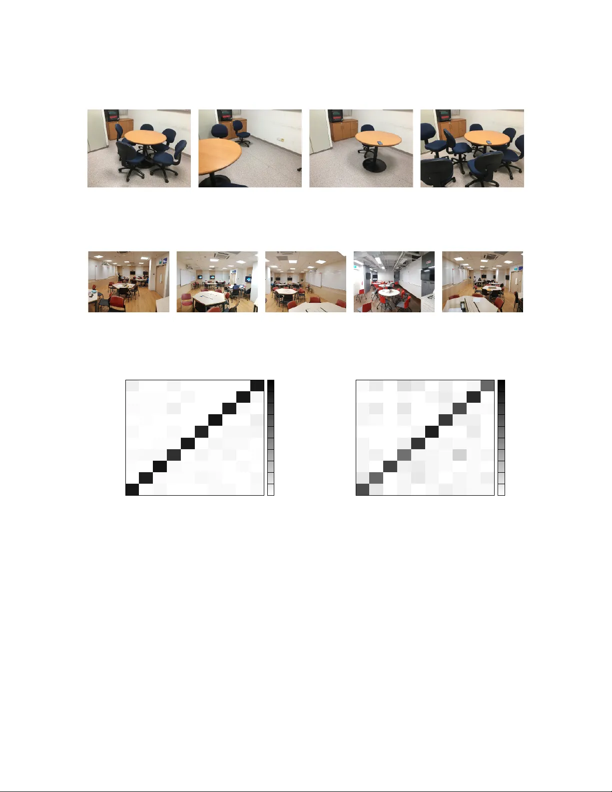
135 Deep Room Recognition Using Inaudible Echos QUN SONG, Energy Research Institute , Interdisciplinary Graduate School, Nanyang T echnological University , Singapore and School of Computer Science and Engineering, Nanyang T echnological University , Singap ore CHA OJIE GU, Scho ol of Computer Science and Engineering, Nanyang T echnological University , Singap ore RUI T AN, School of Computer Science and Engineering, Nanyang T e chnological University , Singapore Recent years have seen the increasing need of location awareness by mobile applications. This paper presents a room-level indoor localization approach based on the measured room’s echos in response to a two-millisecond single-tone inaudible chirp emitted by a smartphone ’s loudspeaker . Dierent from other acoustics-based room recognition systems that record full-spectrum audio for up to ten seconds, our approach records audio in a narrow inaudible band for 0.1 seconds only to preserve the user’s privacy . Howev er , the short-time and narro wband audio signal carries limited information about the room’s characteristics, presenting challenges to accurate room recognition. This paper applies deep learning to eectively capture the subtle ngerprints in the rooms’ acoustic responses. Our extensive experiments show that a tw o-layer convolutional neural network fed with the spectrogram of the inaudible echos achieve the best performance, compar ed with alternative designs using other raw data formats and deep mo dels. Based on this result, we design a RoomRe cognize cloud service and its mobile client library that enable the mobile application developers to readily implement the room recognition functionality without resorting to any e xisting infrastructures and add-on hardwar e. Extensive evaluation sho ws that RoomRecognize achieves 99.7%, 97.7%, 99%, and 89% accuracy in dierentiating 22 and 50 residential/oce rooms, 19 spots in a quiet museum, and 15 spots in a crowded museum, respectively . Compared with the state-of-the-art approaches based on support vector machine, RoomRecognize signicantly improves the Pareto frontier of recognition accuracy versus robustness against interfering sounds (e.g., ambient music). CCS Concepts: • Human-centered computing → Smartphones ; • Computing methodologies → Supervise d learning by classication ; Additional K ey W ords and Phrases: Room recognition, smartphone, inaudible sound A CM Reference Format: Qun Song, Chaojie Gu, and Rui Tan. 2018. Deep Room Recognition Using Inaudible Echos. Proc. ACM Interact. Mob. W earable Ubiquitous T echnol. 2, 3, Article 135 (Septemb er 2018), 29 pages. https://doi.org/10.1145/3264945 1 IN TRODUCTION Recent years have seen the increasing need of location awareness by mobile applications. As of November 2017, 62% of the top 100 free Android Apps on Google P lay require location ser vices. While GPS can provide outdoor locations with satisfactory accuracy , determining indoor locations has b een a hard problem. Resear ch in the last decade has proposed a plethora of indoor lo calization approaches that use various signals such as Wi-Fi [ 8 , 18 ], GSM [ 20 ], FM radio [ 10 ], geomagnetism [ 11 ], and aircraft ADS-B messages [ 15 ]. These systems aim at achieving meters to centimeters localization accuracy . Dierently , this paper aims to design a practical A uthors’ addresses: Qun Song, song0167@e.ntu.edu.sg; Chaojie Gu, gucj@ntu.edu.sg; Rui Tan, tanrui@ntu.edu.sg, School of Computer Science and Engineering, Nanyang T e chnological University , Block N4 #02a-32, 50 Nanyang A venue, Singapore 639798. Permission to make digital or hard copies of all or part of this work for personal or classroom use is grante d without fe e provided that copies are not made or distributed for prot or commercial advantage and that copies bear this notice and the full citation on the rst page. Copyrights for components of this work o wned by others than ACM must be honored. Abstracting with cr edit is permitted. T o copy otherwise, or republish, to post on servers or to redistribute to lists, requires prior specic permission and /or a fee. Request permissions from permissions@acm.org. © 2018 Association for Computing Machinery . 2474-9567/2018/9- ART135 $15.00 https://doi.org/10.1145/3264945 Proc. ACM Interact. Mob. W earable Ubiquitous T echnol., V ol. 2, No. 3, Article 135. Publication date: September 2018. 135:2 • Q . Song et al. room-level lo calization approach for o-the-shelf smartphones using their built-in audio systems only . Room-level localization is desirable in a range of ubiquitous computing applications. For instance, in a hospital, kno wing which room that a patient is in is important to r esponsive medical aid when the patient develops an emergent condition (e.g., falling in a faint). In a museum, knowing which exhibition chamber that a tourist is in can largely assist the automation of her multimedia guide that is often provided as a mobile App nowadays. In a smart building, the room-level localization of the residents can assist the automation of illumination and air conditioning to improve energy eciency and occupant comfort. The requirements of existing indo or lo calization approaches can be summarized as: ( R1 ) a dedicated or an existing infrastructure that pro vides signals for localization [ 10 , 18 , 20 ]; ( R2 ) add-on e quipment to the user’s smartphone [ 15 ]; and/or ( R3 ) a training process to collect data for the subsequent localization processes [ 11 , 18 ]. Any of the above three requirements leads to a certain degree of ov erhead in deploying the indoor localization services. How ever , most existing approaches have at least one of the above drawbacks. In respect of the requirements R1 and R2 , as our approach is base d on the phone’s built-in audio only , it does not require any infrastructure and add-on equipment to the phone. If eective acoustic r epresentations of the target rooms can be found, acoustics-based room-level localization can be cast into a super vised multiclass classication problem by treating the r ooms as classes. Thus, in respect of the last requirement R3 , we aim to design an acoustics-based room recognition approach with an easy training data collection process. For instance, the system trainer can simply carry a smartphone to the target rooms, click some buttons on the phone screen, and ke y in the room names. Such a process can be easily accomplishe d by non-experts. Thus, compared with other ngerprint-based approaches [ 11 , 18 ] that require pr ecisely controlled training data collection processes at dense locations, the training of our system is practical and nearly eortless. Once trained, for the end users, the room recognition becomes an out-of-the-b ox feature. Some existing indoor localization systems hav e incorporate d acoustic sensing. An early study , SurroundSense [ 7 ], used the acoustic loudness in combination of other sensing modalities such as imaging to distinguish the ambient environments. Howev er , the trials of using acoustics alone have not achieved satisfactor y performance yet. For instance, with acoustics only , SurroundSense outperforms barely random guessing [ 36 ]. Batphone [ 36 ] used the acoustic background spectrum as a featur e to classify rooms. However , it achieves a 69% accuracy only in classifying 33 rooms. Moreover , as it uses the [ 0 , 7 kHz ] audible band, it is inevitably susceptible to foregr ound sounds. As shown in [ 36 ] and this paper , Batphone fails in the presence of chatters and ambient music. Dierent from these systems [ 7 , 36 ] that passively listen to the room’s foreground or background sounds, in this paper , we investigate an active sensing scheme that uses the phone’s loudspeaker to emit a predene d signal and then uses the microphone to capture the reverberation in the measured room. Intuitively , due to dierent sizes of the r ooms and dierent acoustic absorption rates of the wall and furniture materials, the acoustic echos may carr y features for distinguishing rooms. Moreover , as we use an a priori signal to stimulate the room, we can design the signal to minimize the unwanted impacts of other interfering sounds (e.g., ambient music and human conversations) on the room recognition. Howev er , the following two basic requirements present challenges to the design of the active room recognition system. First, lengthy audio recording in private/semi-private spaces (e.g., homes and wards) to capture acoustic features may cause the user’s privacy concern. Therefore, to avoid privacy breach, the audio recording time needs to be minimal. Second, it is desirable to use inaudible sounds with frequencies above 20 kHz as the stimulating signals. This av oids annoyance to the user and well separates the stimulating signals from most man-made audible sounds to improve the system’s r obustness. Moreover , as the performance (e.g., sensitivity ) of most smartphone audio systems decreases drastically with the fr equency b eyond 20 kHz , it is desirable to use a narrowband stimulating signal with a central frequency close to 20 kHz . Therefore , to meet the above two requirements, we should use a short-time narrowband inaudible stimulating signal. However , due to the limited time and frequency spans of the stimulating signal, the responding echos will inevitably carr y limited information ab out Proc. ACM Interact. Mob. W earable Ubiquitous T echnol., V ol. 2, No. 3, Article 135. Publication date: September 2018. Deep Room Recognition Using Inaudible Echos • 135:3 the measured room. As a r esult, extracting features from the echos, which is a key step of supervised classication, to distinguish the rooms becomes challenging. In particular , classication system designers generally handcraft the features, often through exhaustiv e trials of popular features. This ad hoc approach, howev er , is ineective if the distinguishability is intricately embedded in the raw data. The emerging deep learning method [ 26 ] automates the design of feature e xtraction by unsuper vised feature learning and employs deep models with a large number of parameters to eectively capture the intricate distin- guishability in the raw data. Its outperforming performance has be en demonstrated in a number of application domains such as image classication [ 23 ], spee ch recognition [ 21 ], natural language understanding [ 12 ], and etc. Thus, deep learning is a promising method to address the aforementioned challenges caused by the ne ed of using short-time narrowband inaudible stimulating signals in the active sensing scheme. This paper presents the design of a deep room recognition approach through extensiv e experiments investigating appropriate forms of the raw data, the choice of the deep model, and the design of the model’s hyperparameters. The results sho w that a two-layer convolutional neural netw ork (CNN) fed with the spectrogram of the captured inaudible echos achieves the best performance. In particular , based on a 100 ms audio recording after a 2 ms 20 kHz single-tone chirp, the CNN gives 99.7%, 99%, and 89% accuracy in distinguishing 22 r esidential and oce rooms, 19 spots in a quiet museum, and 15 spots in a crowded museum, respectively . Moreover , it scales well with the number of rooms – it maintains a 97.7% accuracy in distinguishing 50 rooms. Our approach signicantly outperforms the passive-sensing-based Batphone [ 36 ] that achieves a 69% accuracy using ten seconds of privacy-breaching audio recording. Moreover , compared with a state-of-the-art active sensing approach based on support vector machine (SVM) [ 31 ], our CNN-based approach signicantly improv es the Pareto frontier of recognition accuracy versus robustness against interfering sounds (e .g., ambient music). Based on these results, we design a cloud service named RoomRecognize that facilitates the integration of our room recognition ser vice into mobile applications. In particular , RoomRecognize supp orts a participatory learning mode where the end users can contribute training data. The contributions of this paper include (i) an in-depth measurement study on the rooms’ acoustic r esponses to a short-time single-tone inaudible chirp, (ii) the design of a deep model that eectively captures the subtle dierences in rooms’ acoustic responses, (iii) extensiv e evaluation of our approach in real-w orld environments including homes, oces, class rooms, and museums, as well as (iv) a room recognition cloud ser vice and its mobile client library that are ready for application integration. The rest of this pap er is organized as follows. Section 2 re views related work. Se ction 3 presents a measurement study to understand rooms’ responses to inaudible chirps. Section 4 presents the design of our deep room recognition system. Sections 5 and 6 design and evaluate RoomRecognize, respectively . Section 7 discusses several issues not addressed in this paper . Section 8 concludes. 2 RELA TED W ORK As a challenging pr oblem, indoor localization has received extensive research. Existing appr oaches are either infrastructure-dependent or infrastructure-free . The infrastructure-dependent approaches leverage existing or pr e- deployed infrastructures to determine the location of a mobile device. Existing radio frequency (RF) infrastructures such as 802.11 [ 8 , 18 ], cellular [ 20 ], FM radios [ 10 ], aircraft automatic dependent surveillance-broadcast (ADS-B) systems [ 15 ], and a combination of multiple schemes [ 14 ] have be en used for indoor localization. The 802.11-based approaches require dense deplo yment of access points (APs). Most RF-based approaches are susceptible to the inevitable uctuations of the received signal strength due to complex signal pr opagation and/or adaptive transmit power controls [ 10 , 18 ]. The reception of ADS-B signals needs special hardware that is not available on commodity mobile devices. Existing studies have also pr oposed to use acoustic infrastructure for indoor localization. W ALRUS [ 9 ] uses desktop computers to emit inaudible acoustic beacons to lo calize mobile devices. Scott and Dragovic Proc. ACM Interact. Mob. W earable Ubiquitous T echnol., V ol. 2, No. 3, Article 135. Publication date: September 2018. 135:4 • Q . Song et al. [ 32 ] use multiple microphones deployed in a space to determine the locations of human sounds such as clicking ngers. Howev er , the dedicated, lab orious deployments of the acoustic infrastructures impede the adoption of these approaches. Infrastructure-free approaches leverage location indicative signals including geomagnetism [ 11 ], imaging [ 13 ], acoustics, and etc. As our work uses acoustics, the follo wing literature survey focuses on the acoustics-based approaches that can be classied into passive and active sensing approaches. The passive acoustic sensing analyzes the ambient sounds only to estimate the mobile device ’s location. SurroundSense [ 7 ] uses multiple phone ’s sensors (microphone, camera, and accelerometer ) to distinguish the ambient environments (e.g., dierent stores in a mall). It uses the loudness as the main acoustic feature. As tested in [ 36 ], with the acoustic modality only , SurroundSense outperforms barely random guessing. Its lengthy acoustic recording and image capture also raises privacy concerns when used in private spaces. Batphone [ 36 ] applies the nearest neighbor algorithm to recognize a room based on the acoustic background spectrum in the [ 0 , 7 kHz ] band. In quiet environments, Batphone achiev es a 69% accuracy in classifying 33 rooms. Howe ver , it is highly susceptible to foreground sounds. Using the [ 0 , 7 kHz ] band, it performs worse than random guessing in the presence of a single human sp eaker . Narrowing the band to [ 0 , 300 Hz ] rescues Batphone to achieve a 63.4% accuracy , but drags the quiet case’s accuracy to 41% [ 36 ]. Thus, Batphone has a poor Pareto frontier of recognition accuracy versus robustness against interfering sounds. The active acoustic sensing uses the phone ’s loudspeaker to emit chirps and the micr ophone to capture the echos of the measured space. This approach has been applied to semantic location recognition [ 16 , 24 , 34 ]. In [ 24 ], a decision tree is trained to classify a phone’s semantic location (e.g., in a backpack, on a desk, in a drawer , etc) using active vibrational and acoustic sensing. The phone emits eight audible multi-tone chirps that cover a frequency range from 0 . 5 kHz to 4 kHz . In [ 16 ], the mel-frequency cepstral coecients (MFCC) [ 41 ] of the acoustic echos triggered by audible sine sweep chirps are used to dete ct whether the phone’s environment is a restroom. In [ 34 ], active acoustic sensing, combine d with other passive sensing using magnetometer and barometer , classies the phone ’s environment into six semantic locations: desk, restr oom, meeting room, ele vator , smoking area, and cafeteria. The classication is base d on a decision tree traine d by the random forest algorithm with MFCC of the audible echos as the acoustic feature. These semantic lo calization approaches are fundamentally dierent from our room recognition approach, in that they give the type of the context only and they do not tell the room’s identity . For instance, the approaches in [ 16 , 34 ] do not dierentiate the restrooms in dierent buildings. Following the active acoustic sensing approach, Echo T ag [ 37 ] determines the phone’s position using SVM among a set of predened positions that are ngerprinted using audible echos. In other words, Echo T ag “remembers” predened p ositions with certain tolerance ( 0 . 4 cm ) and resolution ( 1 cm ). This is dierent from our objective of room recognition. RoomSense [ 31 ] is a system that is the closest to ours. Follo wing the active sensing approach, a RoomSense phone emits an audible sound of 0.68 seconds and classies a room using SVM based on the echos’ MFCC featur es. As RoomSense uses the whole audible band, it is susceptible to ambient sounds. Thus, it demands well controlled conditions, e.g., closed windows and doors [ 31 ]. In contrast, due to the use of narro wband stimulating signal, our approach is much more robust against ambient sounds. In this paper , we conduct experiments to extensively compare our approach with RoomSense and our improved versions of Ro omSense that use narrowband stimulating signals as well. The r esults show that, when the acoustic sensing is restricted to a narr ow inaudible band, our spectrogram-based CNN gives 22% and 17.5% higher recognition accuracy than Ro omSense’s MFCC-based SVM, in the absence and presence of interfering ambient music, respectively . Active acoustic sensing has also been used for ranging, moving obje ct tracking, and gesture recognition. BeepBeep [ 30 ] and SwordFight [ 40 ] measure the distance b etween two phones by acoustic ranging. Recent studies also apply active acoustic sensing to track the movements of a nger [ 38 ], breath [ 28 ], and a human body using inaudible chirps emb edded in music [ 29 ]. However , these studies [ 28 – 30 , 38 , 40 ] address ranging Proc. ACM Interact. Mob. W earable Ubiquitous T echnol., V ol. 2, No. 3, Article 135. Publication date: September 2018. Deep Room Recognition Using Inaudible Echos • 135:5 = L2 Fig. 1. Floor plan of the lab. OA L1 L2 L3 L4 (music) L1 (music) L2 (music) L3 (music) L4 OA L1 L2 L3 L4 Actual room Predicted room 0 0.1 0.2 0.3 0.4 0.5 0.6 0.7 0.8 0.9 1 Fig. 2. Confusion matrix of Batphone [ 36 ] in the lab. and ranging-based moving object tracking, rather than classication. SoundW ave [ 17 ] generates inaudible tones with a commodity device’s built-in speaker and analyzes the Doppler-shifted reections sensed by a built-in microphone to infer various features such as velocity , orientation, proximity , and size of moving hands. Based on these features, SoundW ave recognizes the hand gesture . 3 MEASUREMEN T ST UD Y In this section, we conduct measurements to motivate our study and gain insights for the design of our approach. The measurements are conducted in a computer science lab shown in Fig. 1 . The measured rooms are labeled by “Lx” . The open area of the lab is labele d by “OA ” . 3.1 Performance of Passive Acoustic Sensing As discussed in Section 2 , Batphone is a recent room recognition approach based on passive acoustic sensing. W e install the implementation of Batphone [ 36 ] from Apple’s App Store [ 35 ] on an iPhone 6s. W e test its performance using ve rooms, i.e., L1 to L4, and OA shown in Fig. 1 . W e use the default setting of Batphone to collect training data in each room. Specically , the training data collection in each room takes ten seconds. During the testing phase, we test Batphone for ten times in each r oom, in the morning, afternoon, and evening. Thus, Batphone is tested for each r oom for 30 times totally . Note that the data collection for each test takes ten seconds. As discussed in [ 36 ], Batphone has signicant p erformance drop in the presence of foreground sounds. Thus, in the rst set of tests, we keep quiet envir onment in favor of Batphone during the training and testing phases. The bottom part of Fig. 2 shows Batphone’s confusion matrix in the rst set of tests. When the actual room is OA and L4, Batphone can accurately recognize the two rooms. How ever , when the actual room is L1, L2, or L3, Batphone yields high recognition errors. For example, when the actual room is L2, Batphone gives a 40% accuracy only . A possible reason for such low performance is that, as these rooms are in proximity with each other , they may have similar ambient background spectrum that Batphone relies on. In the se cond set of tests, we evaluate the performance of Batphone in the presence of foreground sounds. Specically , we keep quiet environment during the training phase and play a music sound track on a laptop computer during the testing phase. The top part of Fig. 2 shows Batphone’s confusion matrix in this set of tests. The rooms L1 to L4 are always wr ongly classied as O A. The Proc. ACM Interact. Mob. W earable Ubiquitous T echnol., V ol. 2, No. 3, Article 135. Publication date: September 2018. 135:6 • Q . Song et al. chirp echo Fig. 3. Active acoustic sensing. above two sets of tests show the challenges faced by passive acoustic sensing in real-world environment and its susceptibility to interfering sounds. 3.2 Rooms’ Responses to Single- T one Chirps The results in Se ction 3.1 motivate us to explore active acoustic sensing. Fig. 3 illustrates the active sensing scheme . Specically , the smartphone uses its loudspeaker to emit an acoustic chirp and meanwhile uses its microphone to capture the measured r oom’s response. In this section, we conduct a small-scale measurement study to obtain insightful observations on the rooms’ responses. These observations help us make various design choices for an eective active sensing appr oach in Section 4 . Note that the systematic e valuation on the eectiveness of our active sensing approach will be presented in Section 6 . 3.2.1 Measurement Setup. Our measurement study uses a Samsung Galaxy S7 phone with Android 7.0 Nougat. T o collect data, we develop a program that emits a chirp with a time duration of 2 ms using the phone’s loudspeaker every 100 ms . Meanwhile, the program continuously samples the phone ’s microphone at a rate of 44 . 1 ksps and stores the raw data to the phone’s internal memor y for oine analysis. Thus, the program will capture both the chirps that directly propagate from the loudspeaker and the echos from the room if any . With the setting of 2 ms for the chirp length, the chirp will not o verlap the echos from the objects that are mor e than 34 cm from the phone. By emitting the chirp every 100 ms , in each measured room, we can easily collect a large volume of the room’s acoustic responses to the chirps to drive the design of our deep learning based appr oach. W e set the period to be 100 ms , because from our preliminary measurements, the echos vanish after 100 ms from the chirp. In each room, we randomly select at least two spots. W e place the phone at each sp ot and run the program to collect data for about half an hour . Note that, this half an hour time period is merely for collecting data to understand the rooms’ responses with sucient statistical signicance. The minimum neede d volume of training data for our room recognition system will be investigated in Section 6 . Existing studies on active acoustic sensing often use sine sweep chirp [ 16 ], Maximum Length Sequence [ 31 ], and multi-tone chirp [ 24 ] that cover a wide acoustic spectrum, including the audible range, to increase the information carried by the echos about the measured rooms. However , the audible chirps are annoying. In this paper , we propose to use a single-tone inaudible chirp to avoid the annoyance to the user and also impro ve the robustness of the room recognition system against interfering sounds. From our tests, the performance of the phone’s audio system decr eases with the frequency beyond 20 kHz . Fig. 4 shows the signal recorded by the phone’s microphone when the program emits 20 kHz and 21 . 4 kHz chirps. When the congured frequency is 20 kHz , the received signal does exhibit a 20 kHz frequency . Howe ver , when the congured frequency is 21 . 4 kHz , the received signal is signicantly distorted and b ecomes audible. This is because that the mechanical dynamics of either the loudspeaker or the microphone cannot well support such a high frequency . Fig. 5 shows the pow er of the received signal v ersus the congured frequency . The decreasing trend indicates that the audio system’s Proc. ACM Interact. Mob. W earable Ubiquitous T echnol., V ol. 2, No. 3, Article 135. Publication date: September 2018. Deep Room Recognition Using Inaudible Echos • 135:7 -10000 -5000 0 5000 10000 0 0.5 1 1.5 2 Amplitude Time (ms) 20 kHz -10000 -5000 0 5000 10000 0 0.5 1 1.5 2 Amplitude Time (ms) 21.4 kHz Fig. 4. 20 kHz and 21 . 4 kHz chirps received by the phone ’s microphone. 0 1 2 3 4 5 20.0 20.6 21.2 Signal power Chirp frequency (kHz) Fig. 5. Chirp power . -30000 -20000 -10000 0 10000 20000 30000 0 10 20 30 40 50 60 70 80 90 100 Ampltitude Time (ms) echo data period (a) Acoustic trace in L3 for 100 ms after the beginning of the chirp. -500 -400 -300 -200 -100 0 100 200 300 400 13.8 20 30 40 50 60 70 80 90 100 Amplitude Time (ms) (b) Zoom-in view of the signal in (a) during (13.8, 100) ms. -2000 -1500 -1000 -500 0 500 1000 1500 2000 13.8 20 30 40 50 60 70 80 90 100 Correlation Time (ms) (c) Correlation with the chirp template in L3. -2000 -1500 -1000 -500 0 500 1000 1500 2000 13.8 20 30 40 50 60 70 80 90 100 Correlation Time (ms) (d) Correlation with the chirp template when tested outdo or . Fig. 6. Time-domain responses of room L3 and outdoor . performance decreases with the frequency . Therefore, in this paper , we choose 20 kHz , i.e., the lowest inaudible frequency , for the stimulating signal used by our system. T o check if a smartphone can emit and receive inaudible signals (e .g., the 20 kHz tone used by our approach), utilities such as the Near Ultrasound T ests [ 3 ] provided by the Android Open Source Project and various tone generator and spectrum analyzer Apps in Apple’s App Store can be used. From our tests, recent models of Android phones ( e.g., Samsung Galaxy S7, S8, etc) and iPhone (6s, 7, and X) can well emit and receive the 20 kHz tone used by our approach. 3.2.2 Time-Domain A nalysis. W e analyze the data collected for a chirp in room L3 shown in Fig. 1 . The raw acoustic trace for 100 ms is shown in Fig. 6(a) . The period from the beginning to the rst vertical line is the chirp period of 2 ms . During this period, the acoustic signal pr opagates directly from the phone ’s loudspeaker to its microphone. After the chirp period, we discard the data during 0 . 5 ms as a safeguard region and use the data during the remaining 97 . 5 ms to extract echos. This 97 . 5 ms period is calle d echo data p eriod . From Fig. 1 , we can see that the chirp do es not immediately stop after the 2 ms chirp period. It lasts for several milliseconds with decreasing amplitude. Such damped oscillation can be caused by the me chanical dynamics of the loudspeaker’s Proc. ACM Interact. Mob. W earable Ubiquitous T echnol., V ol. 2, No. 3, Article 135. Publication date: September 2018. 135:8 • Q . Song et al. 0 0.5 1 1.5 2 2.5 3 3.5 19.5 20 20.5 PSD Frequency (kHz) L1 Spot A L1 Spot A (a) Same room, same sp ot, dierent times 0 0.5 1 1.5 2 2.5 3 3.5 19.5 20 20.5 PSD Frequency (kHz) L1 Spot A L1 Spot B (b) Same room, dierent spots 0 0.5 1 1.5 2 2.5 3 3.5 19.5 20 20.5 PSD Frequency (kHz) L1 L2 (c) Dierent rooms Fig. 7. Frequency responses of rooms L1 and L2. (Please view the color version for beer visibility .) and the microphone ’s diaphragms. As the damped oscillation still has much stronger intensity than that in the following time period that contains echos, to facilitate data visualization in this se ction, we discard the acoustic data collected within the rst 13 . 8 ms from the beginning of the chirp and use the data in the remaining p eriod of 86 . 2 ms to investigate the time-domain response of the measured room. Fig. 6(b) shows the zoom-in view of the signal in the echo data period. By comparing Fig. 6(a) and Fig. 6(b) , we can see that the signal in the echo data period is ab out 100 times weaker , in terms of amplitude, than the self-heard chirp. The signal attenuation during propagation and the absorption by the surrounding objects are the main causes of the w eak signals. Thus, we question the presence and salience of the echos in the signal shown in Fig. 6(b) . W e slide a windo w of 2 ms over the echo data period and compute the correlation between the sampled signal in each window and an ideal 20 kHz sine wave template. Fig. 6( c) shows the correlation over time . W e can clearly see wave packets, which indicate the presence of echos. In particular , there are more than ten interleaving strong and weak wave packets, which suggests multiple acoustic bouncebacks in the room. This shows that the phone ’s audio system can capture such intricate processes w ell. Fig. 6(d) plots the correlation obtained outdoor . It do es not show any wave packets, since there ar e no echos. 3.2.3 Frequency-Domain A nalysis. The time-domain analysis shows the presence of indoor echos in response to single-tone chirps. W e conjecture that dierent rooms hav e dierent frequency responses to the chirps. As the fast Fourier transform (FFT) needs x seconds of data to generate a spectrum with a resolution of 1 / x Hz , the resolution of the spectrum based on the data in an echo data period of 97 . 5 ms is 10 . 3 Hz only . T o improve the resolution, we concatenate the data in 40 echo data periods and then apply FFT to achieve a resolution of 0 . 26 Hz . Fig. 7(a) shows the power spectral densities (PSDs) in the frequency range of [ 19 . 5 , 20 . 5 ] kHz for the data collected at the same spot in room L1 at two dierent times, respectively . The PSDs remain stable over time. Fig. 7(b) shows the PSDs for two dierent spots in room L1. W e can see that they are also similar . Fig. 7(c) shows the PSDs for the data collected from r ooms L1 and L2, respectively . Although L1 and L2 have the same size (cf. Fig. 1 ), the materials in them may have dierent acoustic absorption rates. In Fig. 7(c) , L2 has str onger echos than L1. Moreover , the peak frequencies of the L2’s responses are quite dierent from L1’s. The results in Fig. 7 show that the rooms L1 and L2, though with the same size, e xhibit dierent frequency responses. This is indicative of the dierentiability of the rooms based on their frequency responses to single-tone inaudible chirps. Howev er , a total of four seconds will be neede d to collect data for concatenating 40 echo data periods. This will incur privacy concerns and incr ease computation overhead since a total of 172,000 data points need to be processed. It is desirable to minimize the audio recording time to mitigate the potential privacy concerns and reduce computation overhead. In this paper , we inquire the possibility of using an audio record collected during a single echo data p eriod of 97 . 5 ms to recognize a room, since we believe that in general no meaningful private Proc. ACM Interact. Mob. W earable Ubiquitous T echnol., V ol. 2, No. 3, Article 135. Publication date: September 2018. Deep Room Recognition Using Inaudible Echos • 135:9 0 32 64 96 128 160 Time inde x 19486 19657 19828 19999 20170 20341 Frequency(Hz) (a) Ro om L1, Spot A 0 32 64 96 128 160 Time inde x (b) Room L1, Sp ot B 0 32 64 96 128 160 Time inde x 0 2 4 6 8 10 (c) Ro om L1, Spot C 0 32 64 96 128 160 Time inde x 19486 19657 19828 19999 20170 20341 Frequency(Hz) (d) Ro om L2, Spot A 0 32 64 96 128 160 Time inde x (e) Ro om L2, Spot B 0 32 64 96 128 160 Time inde x 0 2 4 6 8 10 (f ) Room L2, Spot C Fig. 8. Spectrograms at dierent spots in dierent rooms. information can be extracted by an inspection on a 97 . 5 ms audio record. A possible approach is to apply FFT on the 4,300 data points in the echo data p eriod to generate a PSD and use the [ 19 . 5 , 20 . 5 ] kHz band to recognize a room. In Section 4 , this short-time PSD is employ ed as a p ossible format of the raw data input to the de ep room recognizer . 3.2.4 Time-Frequency A nalysis. Our measurements in Section 3.2.2 and 3.2.3 show that the bouncebacks of the echos form a process over time. Moreov er , the tested rooms L1 and L2 exhibit distinct fr equency responses. Thus, we investigate whether the spectrogram, a time-frequency representation of the raw data, can characterize a room eectively . Specically , we apply 256-point Hann windows, with 128 points of ov erlap between two neighbor windows, to generate a total of 32 data blocks from the 4,300 data points in the echo data period. W e note that the Hann windowing suppresses the side lobes of the PSD computed by the short-time FFT . The concatenation of all blocks’ PSDs over time forms a spectrogram. A s each PSD has ve points only in the frequency range of interest, i.e., [ 19 . 5 , 20 . 5 ] kHz , the spectrogram that we use is a mono chrome image with a dimension of 32 (time) × 5 (frequency). Fig. 8( a) shows ve concatenated spectrograms corresponding to ve chirps when the phone is placed at spot A in r oom L1. W e can se e that the spe ctrograms exhibit similar patterns. Fig. 8(b) and 8(c) show the results for two other spots, B and C, in room L1. Each spot has similar spectrograms. Moreover , we can observe some dierences among the spectrograms at the thr ee spots. Fig. 8(d) , 8( e) , and 8(f ) show the spectrograms at three spots in room L2. Although the rooms L1 and L2 have the same size and the same furniture ( cf. Fig. 1 ), their spectrograms show perceptible dierences. Specically , each spectrogram in the room L1 consists of tw o or more disjunct segments in time, whereas each spectrogram in the room L2 is a more unied segment. This is b ecause the two rooms’ responses to the chirp have dier ent time-domain characteristics. From the results sho wn in Fig. 8 , the tested rooms L1 and L2, though with the same size and furniture , show distinct echo spectrograms in response to single-tone chirps. This obser vation suggests that it is possible to recognize a room using a short audio record. Howe ver , the spectrograms at dierent sp ots in the same room also exhibit some dierences. Therefore , it is interesting to develop a classier that can dierentiate rooms while remaining insensitive to the small dierences among dier ent spots in the same room. Proc. ACM Interact. Mob. W earable Ubiquitous T echnol., V ol. 2, No. 3, Article 135. Publication date: September 2018. 135:10 • Q . Song et al. 4 DEEP ROOM RECOGNI TION Based on the observations in Se ction 3 , this section presents the design of the deep model for room recognition. Section 4.1 introduces the background of deep learning and states the r esearch problem. Section 4.2 presents a set of preliminary trace-driven experiments to e valuate the performance of Deep Neural Network (DNN) and Convolutional Neural Netw ork (CNN). The results show that CNN outperforms DNN. Section 4.3 designs the hyperparameters of the CNN through a set of experiments. 4.1 Background and Problem Statement The performance of the traditional classication algorithms such as Bayes classiers and SVM highly depends on the eectiveness of the designed feature . The feature design is often through a manual featur e engineering process that exhaustively examines various popular dimension reduction techniques. For instance, in the audio processing landscape, handcrafted MFCC [ 41 ] and Perceptual Linear Predictive (PLP) coecients [ 19 ] are widely used as the basis for audio feature design. The emerging deep learning methods [ 26 ] replace the manual feature engineering process with automated feature learning. Thus, deep learning can substantially simplify the design of the pattern recognition system. More importantly , fe d with sucient training data, deep learning algorithms can eectively capture the intricate r epresentations for feature detection or classication, thus yielding higher recognition accuracy over the traditional classication algorithms. This has b een evidenced by the recent successful applications of deep learning [ 26 ]. DNN and CNN are two types of deep models that are widely used for audio sensing (e.g., speech recognition) and image classication, respectively . A DNN consists of a series of fully connected layers with each layer comprised by a collection of neurons ( or units). The data to be classied initialize the values of the input layer neurons. Multiple hidden layers follow the input layer . The yield of a hidden layer neuron is the output of an activation function that takes the weighted sum of the outputs of all the previous layer’s neurons as input. Thus, a hidden layer neuron is not conne cted with any other neuron in the same layer , but is fully connected to all neurons in the previous layer . In the last layer , i.e., the output layer , the neuron giving the largest value indicates the class of the input data. The training algorithm determines the weights and biases of the neurons to b est t the DNN to the labeled training data. Dierent from DNN that is often used to classify 1-dimensional data, CNN is good at capturing local patterns in data with higher dimensions that largely determine the class of the data. CNN consists of one or more convolutional, pooling, and fully connected (or dense) layers that respectively searches for the local patterns (i.e., featur e extraction), increases the e xtracted feature’s robustness to data translations (e .g., rotation), and votes the classication result. The parameters of the neurons in the convolutional and dense layers are determined in the training process, whereas the pooling layers have no parameters to be trained. The key question we ask in this paper is whether we can recognize a room based on its acoustic response to a 2 ms 20 kHz single-tone chirp. Due to the limited time and frequency spans of the chirp, the r esponse may carry limite d information about the room. T o address this challenge, we apply de ep learning that can capture the dierences deeply embedde d in the raw data of dierent classes. T o this end, we need to design the appropriate format of the raw data, the deep model, and the mo del’s hyp erparameters. These issues will be addressed in Sections 4.2 and 4.3 . 4.2 Design of Raw Data Format and Deep Model 4.2.1 Candidate Raw Data Formats. As shown in Sections 3.2.3 and 3.2.4 , both the frequency-domain and time-frequency representations of the echo data can be indicative of the r ooms’ dierences. Thus, the PSD and spectrogram are two possible raw data formats for deep learning. T o avoid privacy concern, we apply FFT on the 4,300 data points in the echo data period to generate a short-time PSD, rather than concatenating 40 echo data periods as in Se ction 3.2.3 . Then, we only use the 147 points in the [ 19 . 5 , 20 . 5 ] kHz band of the short-time PSD as Proc. ACM Interact. Mob. W earable Ubiquitous T echnol., V ol. 2, No. 3, Article 135. Publication date: September 2018. Deep Room Recognition Using Inaudible Echos • 135:11 conv1 (16 4x4 filters) pooling1 (2x2 filter , stride: 2) conv2 (32 4x4 filters) pooling2 (2x2 filter , stride: 2) dense1 (1024 ReLUs) dense2 ( K ReLUs) 32x5 spectrogram Fig. 9. CNN for room recognition. the input data to a deep model. Following the approach in Section 3.2.4 , the spectrogram for the 4,300 data points has a dimension of 32 (time) × 5 (frequency). Thus, the data volumes of the short-time PSD segment and the spectrogram are similar (i.e., 147 and 160). 4.2.2 Candidate Deep Models. W e implement DNN and CNN using Python based on Google T ensorF low [ 6 ]. The structures and hyperparameters of the deep models are designe d as follows. In Section 4.3 , we will conduct extensive experiments to optimize the hyperparameters. DNN admits one-dimensional inputs only . Thus, the PSD segment can be used directly with the DNN. For the spectrogram, we atten it as a vector with a length of 160 and then use the vector as the input to the DNN. The DNN has two hidden layers with each lay er comprised by 256 rectied linear units (ReLUs). Suppose there are K rooms in the training dataset. The output layer consists of K ReLUs that correspond to the K target classes. Note that the training of ReLU-based neural netw orks is often several times faster than that of the traditional tanh-based and sigmoid-based networks [ 23 , 25 ]. CNN can admit high-dimensional inputs. In what follows, w e describe the design of the CNN that takes the two-dimensional sp ectrogram as the input. A s illustrated in Fig. 9 , the CNN consists of the following layers: conv1 , pooling1 , conv2 , pooling2 , dense1 , and dense2 . The rst four layers extract features from the input data by applying sets of lters that preserve the spatial structure of the input data. The dense layers are equivalent to a DNN that performs classication. These layers are briey explained as follows. • The conv1 layer applies 16 4 × 4 convolution lters to the 32 × 5 spe ctrogram. W e add zero padding to the edges of the input image such that the lter ed image has the same dimension as the input image. A lter is slid over the input image by one pixel each time, yielding a single value in the output image that is computed by an element-wise arithmetic operator . Thus, the conv1 layer generates 16 output images. It further applies the ReLU to rectify the negative pixel values in the 16 output images to zero. This introduces non-linearity that is generally needed by neural networks. • The pooling1 layer performs the max pooling with a 2 × 2 lter and a stride of two to each output image of the conv1 layer . Specically , a 2 × 2 window is slid over the image by two pixels each time, yielding the maximum pixel value in the cov ered 2 × 2 subregion as a pixel of the output image. Thus, the output image has a dimension of 16 × 2 . As pooling downsizes the feature image , it can control o vertting eectively . Proc. ACM Interact. Mob. W earable Ubiquitous T echnol., V ol. 2, No. 3, Article 135. Publication date: September 2018. 135:12 • Q . Song et al. T able 1. A verage accuracy of four possible designs in classifying 22 rooms. PSD segment Spectrogram DNN 19% 80% CNN 33% 99% Moreover , as it generates summary of each subregion, it incr eases the CNN’s robustness to small distortions in the input image. • The conv2 and pooling2 layers p erform similar operations as the conv1 and pooling1 layers, respe ctively . The conv2 layer applies 32 4 × 4 lters with ReLU rectication to generate 32 14 × 2 images. Then, the pooling2 applies max pooling and generates 32 8 × 1 images. These images are attened and concatenated to form a feature vector with a length of 256 ( 8 × 1 × 32 ). • The dense1 layer consists of 1,024 ReLUs. The feature vector fr om the pooling2 layer is fully connected to all these ReLUs. W e apply dropout regulation to avoid overtting and improve the CNN’s performance. Specically , we apply a dropout rate of 0.4, i.e., 40% of the input features will b e randomly abandoned during the training process. • The dense2 layer consists of K ReLUs that corresponds to the K target rooms. For an input spectrogram, the classication result corresponds to the maximum value among the K ReLUs. The above CNN design is for two-dimensional spectrogram. T o use the one-dimensional PSD segment with the CNN, we make the following minor changes to the above design: • The size of the convolution lters in the conv1 and conv2 layers is changed to 1 × 4 . • The size of the lters in the pooling1 and pooling2 layers is changed to 1 × 2 . 4.2.3 Mo del Training. The training process of the DNN and CNN is as follows. W e initialize the neural network’s parameters randomly . For each step of the training, a mini-batch of randomly selected 100 training samples is fed to the neural network. The network performs the forward propagation and computes the cross entropy between the output of the dense2 layer and the one-hot vector formed by the labels of the 100 training samples. The cross entropy is often used as the loss metric to assess the quality of multiclass classication. Based on the cross entropy , stochastic gradient descent is employ ed to optimize the neural network’s parameters ov er many training steps. W e set the learning rate to be 0.001. The training can be stopped when the number of the training steps reaches a predened value or the loss metric does not reduce anymore. 4.2.4 Preliminary Results. T o design the deep room recognition algorithm, we collect 22,000 samples from 22 rooms in three homes, an oce, and the lab shown in Fig. 1 . Each sample is a 100 ms audio record. W e split the data set into three parts: training set, validation set, and testing set. Among 1,000 samples collected from each room, 500, 250, and 250 samples are used as training, validation, and testing data, respectively . In each training-validation ep och, the de ep mo del parameters are tuned by the sto chastic gradient descent based on the training data and the average classication accuracy is computed using the validation data. The epoch is repeated until the average classication err or no longer decreases substantially . The testing data set is used to measure the average classication accuracy of the trained deep model. The testing data is pr eviously unseen by the training-validation phase. In the rest of this pap er , all accuracy results are the average classication accuracy measured using the testing data. On a workstation computer with an Intel X eon E5-1650 processor , 16GB main memory , and a GeForce GTX 1080 Ti graphics processing unit (GP U), the training of the spectrogram-based DNN and CNN achieves the peak validation accuracy after about two minutes. Based on the testing data, the average accuracy of the four p ossible designs in classifying the 22 rooms is shown in T able 1 . From the results, we can see that, although b oth the PSD segment and the spe ctrogram represent Proc. ACM Interact. Mob. W earable Ubiquitous T echnol., V ol. 2, No. 3, Article 135. Publication date: September 2018. Deep Room Recognition Using Inaudible Echos • 135:13 T able 2. The configurations of the teste d CNNs with one to five convolutional layers. CNN- A CNN-B CNN-C CNN-D CNN-E CNN-F CNN-G 1 conv layer 2 conv layers 2 conv layers 2 conv layers 3 conv layers 4 conv layers 5 conv layers 5 × 32 images conv4-16 conv4-16 conv4-16 conv4-32 conv4-16 conv4-16 conv4-16 max pooling n.a. conv4-16 conv4-32 conv4-32 conv4-32 conv4-32 conv4-32 n.a. max pooling n.a. n.a. n.a. n.a. conv4-64 conv4-64 conv4-64 conv4-128 conv4-128 conv4-256 dense-1024 dense- K softmax conv x - n represents a total of n x × x convolution lters; dense- n represents a dense layer with n ReLUs. the same raw data, the deep models fed with the spe ctrogram give much higher classication accuracy . This is because the distinction in the time dimension among the rooms’ responses to the chirps is more salient than the distinction in the frequency dimension. Thus, although the sp ectrogram has a much lower frequency resolution than the PSD segment (i.e., 5 points vs. 147 points), the spectrogram is more eective in expressing the r esponse of a room. Based on the spectrogram, DNN and CNN achieve 80% and 99% classication accuracy , respectively . Although in this preliminary test we do not extensiv ely optimize the hyperparameters of the two deep models, the test result is consistent with the common understanding that CNN is better in classifying images. Thus, in the rest of this paper , we choose the combination of spectrogram and CNN. 4.3 Hyperparameter Seings The results in Se ction 4.2 show that CNN is an appropriate deep mo del for room recognition. This section presents our experiments to decide the settings of the following hyperparameters: the number of convolutional lay ers, the presence of pooling layers, the number of lters in the convolutional lay ers, and the sizes of the lters. In each experiment, we vary a single hyperparameter and keep others unchange d. For each setting, we train and test the CNN using the training-validation and testing samples collecte d from the 22 rooms as describe d in Section 4.2.4 . 4.3.1 The Number of Convolutional Layers. First, we study the impact of the number of conv olutional layers on the classication accuracy . W e follow the test methodology used in the design of the VGG net [ 33 ]. W e test a total of seven CNNs, named fr om CNN- A to CNN-G, with one to ve convolutional layers. The congurations of these CNNs are illustrated in T able 2 , in which “conv x - y ” means a total of y convolutional lters with size of x × x . All convolutional lters use a stride of one pixel and zer o padding. Max pooling with window size of 2 × 2 and stride of two is applie d after some of the convolutional layers. Note that we can apply at most two max pooling layers, since after that the image size reduces to 1 × 8 . All tested CNNs have two dense layers. The rst has 1024 ReLUs, whereas the second consists K -way classication channels for the last soft-max lay er that gives the nal classication result. T able 3 shows the total numb er of the neurons’ parameters, training time on the aforementioned workstation computer , and classication accuracy of dierent CNNs illustrate d in T able 2 . W e note that, as CNN- A has one max pooling layer only and pooling can reduce the size of the images going through the network, CNN- A contains more parameters than CNN-B, C, and D that have tw o convolutional and pooling layers. W e can see Proc. ACM Interact. Mob. W earable Ubiquitous T echnol., V ol. 2, No. 3, Article 135. Publication date: September 2018. 135:14 • Q . Song et al. T able 3. Training time and accuracy of various CNNs. CNN- A B C D E F G The number of parameters (million) 0.48 0.14 0.26 0.26 0.52 1.11 2.55 Training time ( second) 115 112 119 124 134 158 203 Accuracy (%) 93.6 95.7 99.7 95.1 90.2 74.4 58.4 T able 4. Accuracy under various numbers of filters in the two convolutional layers. The number of lters (8, 16) (16, 32) (32, 64) (64, 128) Accuracy (%) 92.1 99.7 96.4 94.8 ( x , y ): x lters in conv1 , y lters in conv2 . The size of the lters is 4 × 4 . that the training time increases with the number of parameters, but the accuracy do es not. The CNN-C with two convolutional lay ers achieves the highest accuracy among the tested CNNs. Moreov er , the accuracy of the CNNs with two convolutional layers (i.e., CNN-B, C, and D) is generally higher than other tested CNNs. W e note that more layers or more parameters unnecessarily lead to b etter accuracy due to p otential overtting. From the results in T able 3 , we adopt two convolutional layers in the r est of this paper . 4.3.2 Presence of Pooling Layers. As discusse d in Section 4.1 , the p ooling layers have no parameters to be trained. But their presence can be decided. As the main function of pooling is to reduce the amount of parameters and computation time , as well as incr ease the CNN’s robustness to data translations, the po oling lay ers can be omitted for input images with relativ ely small dimensions [ 27 ]. Our tests show that, by omitting the pooling lays, the accuracy of the CNN increases from 99.7% to 99.9%, probably due to the small dimensions of the spectrogram. Howev er , the omission results in tripled training time. A s long training times are undesirable when our room recognition system runs in a participator y learning mode (cf. Section 5 ), the 0.2% accuracy gain is not worth. Thus, we retain the pooling layers. 4.3.3 The Number and Size of Filters. W e vary the numbers of the lters in the two convolutional layers by looping through the powers of 2 from 16 to 256. T able 4 shows the resulting accuracy . Note that conv2 has doubled lters compared with conv1 . This is a typical setting adopted in many CNNs (e.g., V GG net [ 33 ] and DenseNet [ 22 ]). When conv1 and conv2 have 16 and 32 lters, the CNN gives the highest accuracy . This is because more lters lead to mor e parameters, but unnecessarily better accuracy due to potential overtting. Thus, we adopt 16 and 32 lters for the two layers in our appr oach. W e also test the impact of the lter size on the CNN’s accuracy by varying the size from 2 × 2 to 5 × 5 . T able 5 shows the resulting accuracy . Similarly , the accuracy is concave to the lter size due to potential overtting. In particular , the lter size 4 × 4 gives the highest accuracy . 4.3.4 The Number of Dense Layers. W e var y the number of dense layers from one to three. The last dense layer has K ReLUs, wher eas each of prior dense layers has 1,024 ReLUs. Each dense layer adopts dropout. T able 6 shows the resulting number of neurons’ parameters, training time, and accuracy . W e can see that the conguration of two dense layers as illustrated in T able 2 needs the least training time and gives the highest accuracy . Thus, we adopt two dense layers. 4.3.5 Summary and Discussions. From the above results, the hyperparameter settings for CNN adopted in Section 4.2.2 , i.e., CNN-C shown in T able 3 , are preferable. Thus, w e design our room recognition approach based Proc. ACM Interact. Mob. W earable Ubiquitous T echnol., V ol. 2, No. 3, Article 135. Publication date: September 2018. Deep Room Recognition Using Inaudible Echos • 135:15 T able 5. Accuracy under various filter sizes. Filter size (pixel) 2 × 2 3 × 3 4 × 4 5 × 5 Accuracy (%) 96.9 99.2 99.7 96.8 16 and 32 lters in conv1 and conv2 , respectively . T able 6. Accuracy under various depth of dense layers. Number of dense layers 2 3 4 Number of parameters (million) 0.26 1.3 2.3 Training time (minute) 2 3 4 Accuracy (%) 99.7 98.9 99.1 on CNN-C. W e now discuss two issues rele vant to hyperparameter design. First, although the hyperparameter settings are designed based on the data collected from 22 rooms, in Section 6 , we will evaluate the performance of CNN-C in classifying more r ooms and other types of spaces such as location spots in museums. The results show that CNN-C yields excellent/good classication accuracy in all evaluation cases. Second, more systematic techniques such as grid search and A utoML [ 1 ] can be employed to further optimize the hyperparameter settings. Howev er , since our design experiments have achieved an accuracy of 99.7%, the accuracy improvement by these hyperparameter optimization techniques will not be substantial. W e leave the integration of these techniques when massive training data is available to our future work. 5 DEEP ROOM RECOGNI TION CLOUD SERVICE 5.1 System Overview Based on the results in Section 4 , we design Ro omRecognize , a cloud ser vice for room recognition, and its mobile client library . RoomRecognize, running on a cloud server with GP U support, classies the e cho data sent from a mobile client. With the mobile client librar y , the application developer can readily integrate the cloud service into mobile applications that need room r ecognition ser vices. Fig. 10 shows the architectures of RoomRecognize and its client librar y . In particular , we design Ro omRecognize to support a participatory learning mode, in which the CNN is retrained when a mobile client uploads labeled training samples. Fig. 11 shows the workow of the participatory learning mo de. First, the client collects training samples in a room and uploads to the ser ver . Then, the server will run the current CNN using the training samples and return a list of the most probable r oom labels to the client. The user of the client can check the list. If the current room is not in the list, the user can create a new label and trigger the ser ver to retrain the CNN; otherwise, the uploaded training samples should b e labeled using an existing r oom label before being used for future CNN retraining. This design helps pr event multiple dierent labels dened by the users for the training data collected from the same room. W e note that existing studies [ 25 , 39 ] have shown that smartphones and even lower-end Internet of Things platforms can run deep models. In RoomRecognize, as the transmission of an audio record of 0.1 seconds causes little overhead to today’s communication networks, we choose to run the trained CNN at the cloud server . This design choice also avoids the complications in synchronizing the latest deep model to each client in the participatory learning mode. 5.2 RoomRecognize Ser vice W e build RoomRecognize base d on F lask [ 2 ], a Python-based micro w eb framew ork. Thus, we can easily integrate the Python-based T ensorFlow into Flask. W e use the Flask-RESTful extension to dev elop a set of representational state transfer (RESTful) APIs over H T TPS. Note that RESTful APIs can largely simplify the interoperations between the cloud service and the non-browser-based client programs. Thr ough these APIs, the client can upload an audio record of 0.1 seconds and obtain room recognition r esult, or training samples of multiple labeled audio records. The functionality of these APIs will be further explained in Section 5.3 . The Signal Processing module shown in Fig. 10 extracts the spectrograms from the received audio records. The T ask Monitor manages the Proc. ACM Interact. Mob. W earable Ubiquitous T echnol., V ol. 2, No. 3, Article 135. Publication date: September 2018. 135:16 • Q . Song et al. RESTful A PI W eb Se rver (F lask) Cloud T ensorFlow CNN Recogn ition T raining Fig. 10. Architecture of RoomRecognize. 1.Client uploads training samples Client Server 2.Server returns a list of predicted 3. Client decides whether to add a new room. Server merges training data and retrain. Client uploads a new label, server retrains the CNN. for a measured room to cloud server . room labels using the current CNN. No Y es Fig. 11. W orkf low of participatory learning. training of the CNN with newly received training data in the participatory learning mode. A s the CNN training is performed by a separate process, it will not block the room recognition service. Once the training completes, the deep model is updated. All modules of RoomRecognize are implemented using Python. In this work, we deploy ed the RoomRecognize service to a server equipped with an Intel Core i7-6850K CP U, 64GB main memory , a Quadro P5000 and two GeForce GTX 1080 Ti GP Us. 5.3 RoomRecognize Client Librar y W e design an Android client librar y in Java to wrap the RESTful APIs provided by the RoomRe cognize cloud service. A similar library can b e designed for iOS. The library provides the following methods: • EmitRecord(mode) : This method uses the phone’s loudspeaker to transmit single-tone chirps and micr o- phone to capture the echos. The mode can be either recognition or training . In the recognition mode, the phone emits a chirp only and r ecords audio for 0.1 seconds. In the training mode, the phone r epeats the above emit-record process for 500 times ov er 50 seconds. This is be cause that our evaluation in Section 6 shows that 500 training samples are sucient to characterize a room. This EmitRecord method returns the recorded data to the user program. • UploadData(mode) : In the recognition mode , this method uploads the audio record to the cloud service and obtains the recognition result of a single room label. In the training mode, it uploads the training samples and receives a list of at most v e predicted rooms computed by the cloud service that have the highest neuron values in the CNN’s dense2 layer . In other words, these ve pr edicted rooms are those in the server’s training database that best match the currently measured room. • UploadLabel(label) : This method should be use d in the training mode only . The client can use this method to notify the server the label of the currently measured room. The lab el can be one within the list returned by the UploadData() method, or a new label. For the former case, the server will merge the training samples contribute d by this client using the UploadData() method with the existing training samples from the same room; for the latter case, the server will create a new class and increase the K value by one. Thereafter , the ser ver’s T ask Monitor will trigger a retraining. Note that, in our design, we separate the processes of uploading training data and lab el. This allows the application developer to easily deal with a situation wher e the end user contributes training data collected fr om a room that has been covered by the current training database. Specically , the client program prompts the end Proc. ACM Interact. Mob. W earable Ubiquitous T echnol., V ol. 2, No. 3, Article 135. Publication date: September 2018. Deep Room Recognition Using Inaudible Echos • 135:17 (a) Bedroom (b) Museum hall (c) Visitor oce L1 (d) Lab open area (e) Meeting room L4 Fig. 12. Examples of several room types. user to check whether the current room is within the list returned by the UploadData method and then uploads the label based on the user’s choice. 6 PERFORMANCE EV ALU A TION Using the client librar y described in Section 5 , we have implemented an Android App to use the Ro omRecognize service. In this section, we conduct a set of experiments using the Android App to evaluate the performance of RoomRecognize. 6.1 Evaluation Methodology Section 3.1 has shown the low performance of passive acoustic sensing, and its susceptibility to interfering sounds. In this section, we only compare RoomRecognize with other room recognition approaches that are based on active acoustic sensing. As discussed in Section 2 , active acoustic sensing has been applied to recognize semantic locations [ 16 , 24 , 34 ] and remember predened positions with centimeter resolution [ 37 ]. However , these studies do not address room recognition. Thus, they are not comparable with RoomRecognize. In our evaluation, we compare RoomRecognize with RoomSense [ 31 ]. T o the best of our knowledge, Ro omSense is the only active acoustic sensing system for room recognition. Ro omSense employs the maximum length sequence (MLS) measurement technique to generate chirps in a wide spe ctrum including the audible range, and then classies a room using SVM based on MFCC features. W e implement RoomSense by following the descriptions in [ 31 ]. Specically , w e use Co ol Edit Pro 2.1 to generate the MLS signal. W e follow the measurement approach described in Section 3.2.1 , except that the phone replays the MLS signal, to collect the rooms’ r esponses. With the Python libraries python_speech_features [ 4 ] and scikit-learn [ 5 ], we implement RoomSense’s MFCC feature extraction and SVM-based classication. W e also implement two variants of RoomSense. These two Ro omSense variants emit the single-tone chirps describ ed in Section 3.2.1 instead of MLS signals, and then still apply the MFCC extraction and SVM classication pipeline to classify rooms. The rst RoomSense variant, named single-tone broadband-MFCC RoomSense , sets the lowest and highest band edges for the MFCC extraction to be 0 kHz and 22 . 05 kHz , same as the original setting of RoomSense. The second RoomSense variant, named single-tone narrowband-MFCC RoomSense , sets the two band edges to be 19 . 5 kHz and 20 . 5 kHz . Thus, the single-tone narrowband-MFCC RoomSense and RoomRecognize extract acoustic features from the same frequency band. The comparisons among the RoomRecognize, the original RoomSense, and the two variants of RoomSense will provide insights into understanding the major factors contributing to RoomRecognize’s high classication accuracy . W e conduct experiments in various types of rooms. T able 7 summarizes all the residential, oce , teaching, and museum rooms involv ed in our evaluation. W e note that the design of the CNN hyperparameters, as presented in Section 4.3 , is performed based on the data collected from the rst 22 rooms summarized in T able 7 , excluding the teaching rooms and museum halls. Fig. 12 shows the pictures of sev eral types of rooms. Proc. ACM Interact. Mob. W earable Ubiquitous T echnol., V ol. 2, No. 3, Article 135. Publication date: September 2018. 135:18 • Q . Song et al. T able 7. Descriptions of residential, oice, teaching, and museum rooms involved in our evaluation. Room type Number Size # of spots W all Floor Ambient of rooms (m 2 ) per room material material envir onment Bedroom 9 10-20 2-3 concrete laminated/ceramic generally quiet Living room 2 25-30 3 concrete marble slightly noisy Bathroom 3 15-20 2-3 ceramic ceramic quiet Kitchen 2 10-15 2 ceramic ceramic generally quiet Faculty oce 1 15 2 concrete ceramic quiet Visitor oce (L1) 1 10 2 concrete ceramic slightly noisy Visitor oce (L2) 1 10 2 concrete ceramic quiet Meeting room (L3) 1 7 2 concrete ceramic quiet Meeting room (L4) 1 30 3 concrete ceramic quiet Lab open area 1 150 3 concrete ceramic slightly noisy T eaching room 10 40 1 concrete laminate d quiet Museum- A hall areas 19 15-150 2-3 concrete ceramic slightly noisy Museum-B hall areas 15 30-100 2-3 concrete ceramic noisy , crowded R1 R2 R3 R4 R5 R6 R7 R8 R9 R10 R11 R12 R13 R14 R15 R1 R2 R3 R4 R5 R6 R7 R8 R9 R10 R11 R12 R13 R14 R15 Actual room Predicted room 0 0.1 0.2 0.3 0.4 0.5 0.6 0.7 0.8 0.9 1 (a) No ambient music R1 R2 R3 R4 R5 R6 R7 R8 R9 R10 R11 R12 R13 R14 R15 R1 R2 R3 R4 R5 R6 R7 R8 R9 R10 R11 R12 R13 R14 R15 Actual room Predicted room 0 0.1 0.2 0.3 0.4 0.5 0.6 0.7 0.8 0.9 1 (b) With ambient music Fig. 13. Confusion matrices of the original RoomSense. 6.2 Evaluation Results in Residential, Oice, and T eaching Rooms 6.2.1 Susceptibility to Interfering Sounds. W e evaluate the susceptibility of dierent room recognition approaches to interfering sounds. This set of experiments is conducted in 15 rooms chosen from the rooms listed in T able 7 . W e choose 4 bedrooms, 2 living rooms, 2 kitchens, 3 bathrooms, 2 visitor oces, and 2 me eting rooms. Note that in other rooms it is inconvenient or not allowed to play interfering sounds. In the experiment, we keep the rooms quiet when we collect training data for RoomRecognize, RoomSense, and its variants. When we test their recognition accuracy , we either keep the rooms quiet or play music using a laptop computer in the tested rooms. Figs. 13(a) and 13(b) show the confusion matrices of the original RoomSense in the absence and presence of music, respectively . The respective average r ecognition accuracy is 76% and 39%. Figs. 14(a) and 14(b) show Proc. ACM Interact. Mob. W earable Ubiquitous T echnol., V ol. 2, No. 3, Article 135. Publication date: September 2018. Deep Room Recognition Using Inaudible Echos • 135:19 R1 R2 R3 R4 R5 R6 R7 R8 R9 R10 R11 R12 R13 R14 R15 R1 R2 R3 R4 R5 R6 R7 R8 R9 R10 R11 R12 R13 R14 R15 Actual room Predicted room 0 0.1 0.2 0.3 0.4 0.5 0.6 0.7 0.8 0.9 1 (a) No ambient music R1 R2 R3 R4 R5 R6 R7 R8 R9 R10 R11 R12 R13 R14 R15 R1 R2 R3 R4 R5 R6 R7 R8 R9 R10 R11 R12 R13 R14 R15 Actual room Predicted room 0 0.1 0.2 0.3 0.4 0.5 0.6 0.7 0.8 0.9 1 (b) With ambient music Fig. 14. Confusion matrices of single-tone broadband-MFCC RoomSense. R1 R2 R3 R4 R5 R6 R7 R8 R9 R10 R11 R12 R13 R14 R15 R1 R2 R3 R4 R5 R6 R7 R8 R9 R10 R11 R12 R13 R14 R15 Actual room Predicted room 0 0.1 0.2 0.3 0.4 0.5 0.6 0.7 0.8 0.9 1 (a) No ambient music R1 R2 R3 R4 R5 R6 R7 R8 R9 R10 R11 R12 R13 R14 R15 R1 R2 R3 R4 R5 R6 R7 R8 R9 R10 R11 R12 R13 R14 R15 Actual room Predicted room 0 0.1 0.2 0.3 0.4 0.5 0.6 0.7 0.8 0.9 1 (b) With ambient music Fig. 15. Confusion matrices of single-tone narrowband-MFCC RoomSense. the confusion matrices of the single-tone br oadband-MFCC RoomSense in the absence and presence of music, respectively . The respe ctive average r ecognition accuracy is 83% and 27%. Figs. 15( a) and 15(b) sho w the confusion matrices of the single-tone narrowband-MFCC RoomSense in the absence and pr esence of music, respectively . The respective average recognition accuracy is 69% and 50%. Figs. 16( a) and 16( b) show the confusion matrices of RoomRecognize in the absence and presence of music, respectively . The respe ctive average recognition accuracy is 100% and 81%. In Figs. 13 , 14 , and 15 , the rooms R1-R4 are from a lab; the rooms R5-R10 and R11-R15 are fr om two dierent apartments. From Fig. 13(a) and Fig. 14( a) , we can see some confusion blocks lumping together , e.g., the blocks representing R7-R10 and R13-R14 in Fig. 13(a) and R7-R10 in Fig. 14(a) . This shows that the original RoomSense and the single-tone broadband-MFCC RoomSense make wrong classications for the rooms from the same apartments. It suggests that these two approaches cannot well dierentiate the rooms with similar oor and Proc. ACM Interact. Mob. W earable Ubiquitous T echnol., V ol. 2, No. 3, Article 135. Publication date: September 2018. 135:20 • Q . Song et al. R1 R2 R3 R4 R5 R6 R7 R8 R9 R10 R11 R12 R13 R14 R15 R1 R2 R3 R4 R5 R6 R7 R8 R9 R10 R11 R12 R13 R14 R15 Actual room Predicted room 0 0.1 0.2 0.3 0.4 0.5 0.6 0.7 0.8 0.9 1 (a) No ambient music R1 R2 R3 R4 R5 R6 R7 R8 R9 R10 R11 R12 R13 R14 R15 R1 R2 R3 R4 R5 R6 R7 R8 R9 R10 R11 R12 R13 R14 R15 Actual room Predicted room 0 0.1 0.2 0.3 0.4 0.5 0.6 0.7 0.8 0.9 1 (b) With ambient music Fig. 16. Confusion matrices of RoomRecognize. T able 8. The average classification accuracy of dierent approaches in the absence and presence of music. Approach In the absence of music In the presence of music Original RoomSense 76% 39% Single-tone broadband-MFCC RoomSense 83% 27% Single-tone narrowband-MFCC RoomSense 69% 50% RoomRecognize 100% 81% wall materials. In Fig. 15(a) we can see that the confusion blocks are more disperse d, which means that the single-tone narrowband-MFCC RoomSense is better at recognizing rooms with similar furnishing materials. A possible reason for this impr ovement is that the narrowband-MFCC featur es carry less information about the tested room’s furnishing material. When the ambient music is present, the confusion blocks appear randomly in Figs. 13(b) , 14(b) , and 15( b) . This is be cause the ambient music is the main reason of the confusion. T able 8 summarizes the average recognition accuracy of dierent approaches in the absence and pr esence of music during the testing phase. From Table 8 , the original RoomSense and the single-tone broadband-MFCC RoomSense yield similar accuracy proles. Note that b oth approaches use broadband-MFCC features. By narrow- ing the frequency band of the MFCC features to [ 19 . 5 , 20 . 5 ] kHz , the single-tone narrowband-MFCC RoomSense achieves much b etter recognition accuracy in the presence of music. These comparisons show that using a narrow frequency band can signicantly improv e the system’s robustness to interfering sounds. The single-tone narrowband-MFCC RoomSense performs worse than the other two RoomSense appr oaches in the absence of music. This is be cause the narrowband-MFCC features carry less information about the measured room than the broadband-MFCC features. Fr om these results, we can see that the SVM used by RoomSense can hardly achiev e a satisfactory Pareto frontier of recognition accuracy v ersus robustness against interfering sounds. Specically , on one hand, due to the inferior learning capability , SVM needs echos in a broader frequency band to achieve a satisfactory r ecognition accuracy; on the other hand, the use of broadband audio will inevitably increase the system’s susceptibility to interfering sounds. RoomRecognize has a 19% accuracy drop in the presence of music, because the music may contain frequency components up to 20 kHz . Howev er , compared with the SVM-based Proc. ACM Interact. Mob. W earable Ubiquitous T echnol., V ol. 2, No. 3, Article 135. Publication date: September 2018. Deep Room Recognition Using Inaudible Echos • 135:21 T able 9. Accuracy in recognizing 22 rooms under various training data volumes. V olume of training data for each room (samples) 100 250 375 437 500 Training data collection time for each room ( seconds) 10 26 39 45 52 Room recognition accuracy (%) 83.15 90.5 91.3 94.5 99.7 T able 10. Seing of data collection process for evaluating the impact of phone’s position and orientation. Room Size (m 2 ) Number Number of phone of spots orientations at each sp ot L1 10 6 6 L2 10 6 6 L3 12 8 6 L4 26 16 6 T able 11. Seing of the leave-one-spot-out cross validation. x -1 means that x spots for training and one spot for testing. Spot density (m − 2 ) 1 / 2 1 / 4 1 / 6 1 / 8 1 / 10 Room L1 5-1 3-1 2-1 1-1 1-1 L2 5-1 3-1 2-1 1-1 1-1 L3 6-1 3-1 2-1 2-1 1-1 L4 13-1 7-1 4-1 3-1 3-1 30 40 50 60 70 80 1/101/8 1/6 1/4 1/2 Accuracy (\%) Spot density (m −2 ) Fig. 17. Leave-one-spot-out recognition accuracy vs. spot den- sity for collecting training data. T able 12. Confusion matrix of leave-one- orientation-out cross validation. A verage accuracy is 64%. Predicted room L4 L3 L2 L1 Actual room L4 0.65 0.14 0.11 0.10 L3 0.15 0.60 0.10 0.15 L2 0.03 0.14 0.61 0.22 L1 0.04 0.03 0.23 0.70 RoomSense, RoomRecognize gives a much improv ed Pareto frontier , owing to deep learning’s strong ability to capture subtle dierences in rooms’ narro wband responses. W e note that the 81% average accuracy achieved by RoomRecognize in the presence of ambient music can be considered a worst-case result, because we introduce the interfering sounds in every room during the testing phase. 6.2.2 Ne eded Training Data V olume. Due to the deep models’ massive parameters, a sucient amount of training samples are critical to avoid overtting. Fortunately , for the acoustics-based room recognition problem, the nearly automated training data colle ction process that repeatedly emits chirps and capture the room’s e chos can generate many training samples easily . This set of experiments evaluates the needed training data volume. T able 9 shows the volume of training data for each room, the corresponding training data collection time, and the resulting accuracy in r ecognizing 22 rooms. W e can see that, with 500 samples collected during 52 seconds in each room, the accuracy reaches 99.7%. Proc. ACM Interact. Mob. W earable Ubiquitous T echnol., V ol. 2, No. 3, Article 135. Publication date: September 2018. 135:22 • Q . Song et al. 6.2.3 Impact of P hone Position and Orientation. W e conduct a set of experiments in four rooms (L1 to L4 shown in Fig. 1 ) to evaluate the impact of the phone ’s position and orientation on the performance of RoomRecognize. Specically , we colle ct data using a phone at a total of 37 spots in the four rooms. The spots in a r oom are sele cted such that they are nearly evenly distributed in the room. At each spot, we colle ct 500 samples for each of six phone’s orientations that are perpendicular to each other , i.e., front, back, left, right, up, and down. T able 10 summarizes the settings of the data collection process. In the rst set of experiments, w e conduct leave-one-spot-out cross validation to e valuate the impact of phone position on the performance of RoomRecognize. Specically , out of a total of n spots, we use the data collected at n − 1 spots for training and the data colle cted at the remaining one spot for testing. Thus, the tested spot is not within the training data. W e also var y n to investigate the impact of the sp ot density for collecting training data (i.e., 1 /( 1 − n ) m − 2 ) on the performance of RoomRecognize. T able 11 summarizes the settings of the leave-one-spot-out cr oss validation experiments under dierent spot densities. In the leave-one-spot-out experiments, we consistently use the front orientation for the phone . Fig. 17 sho ws the av erage leave-one-spot-out recognition accuracy versus the spot density for collecting training data. W e can se e that the r ecognition accuracy increases with the spot density . This means that, collecting training samples at more spots in each room will improve the performance of RoomRecognize, which is consistent with intuition. T wo additional comments can be made regarding the results in Fig. 17 . First, the leave-one-spot-out recognition accuracy is below 80% when the spot density is up to 0.5 spot/ m 2 . As we select the spots ev enly in each r oom, the leave-one-spot-out accuracy is the worst-case recognition accuracy (i.e., a lo wer bound) with respect to the impact of phone ’s p osition. Second, the number of spots in each room as summarize d in T able 10 achieve the spot density of 0.5 sp ot/ m 2 . Collecting data at sev eral spots (e .g., 6 to 8 sp ots as in Table 10 ) in rooms with sizes of about 10 m 2 does not introduce signicant overhead to the system trainer . While evenly selecting these spots is certainly preferred, at the end of this section, we will conduct another set of experiments in which the training data is collecte d when the phone carrier walks freely in each room. Then, we evaluate the impact of phone orientation on RoomRe cognize’s performance by conducting a set of leave-one-orientation-out cross validation experiments. The data collected at all sp ots is used for training. T able 12 shows the confusion matrix of the leave-one-orientation-out cross validation. The average recognition accuracy is 64%. This result sho ws that the phone orientation has larger impact on RoomRecognize, compared with the phone position. Note that the leave-one-out accuracy is the worst-case accuracy . By simply colle cting training data for each of the six phone orientations, the worst case can be avoided. In the third set of experiments, we assess RoomRecognize’s performance when the phone carrier walks freely in the measured rooms and rotate the phone randomly during walking. Out of totally 1,000 samples colle cted during a two-minute free walk in each room, 500, 250, and 250 samples are used for training, validation, and testing, respectively . The average room recognition accuracy is 87%. This result shows that RoomRecognize can achieve a satisfactory recognition accuracy without imposing strict requirements to the training data collection process. The system trainer can follow a general guideline of walking in the walkable areas of a room and rotating the phone randomly during the training data collection process. 6.2.4 Scalability . In Section 4.3 , we designed CNN-C based on data collecte d from 22 rooms. In this section, we evaluate how well CNN-C can scale with the number of rooms (i.e ., the number of classes). W e collect data from additional 28 rooms. Thus, we have data from a total of 50 rooms. Among 1,000 samples collecte d fr om each room, 500, 250, and 250 samples are included into the training, validation, and testing data sets, r espectively . Fig. 18 shows the average test accuracy v ersus the number of rooms. W e can se e that the test accuracy decreases with the number of rooms, which is consistent with intuition. Howe ver , RoomRecognize still gives a 97.7% accuracy in classifying 50 rooms. The scale of 50 rooms is satisfactory for a range of application scenarios, i.e ., recognizing museum exhibition chambers, wards of a hospital department, etc. Proc. ACM Interact. Mob. W earable Ubiquitous T echnol., V ol. 2, No. 3, Article 135. Publication date: September 2018. Deep Room Recognition Using Inaudible Echos • 135:23 97 97.5 98 98.5 99 99.5 100 22 30 40 50 Test accuracy (%) The number of rooms Fig. 18. T est accuracy vs. number of rooms. 0 20 40 60 80 100 0 1 2 3 4 Recognition rate (%) Number of moving individuals Fig. 19. Recognition rate vs. the number of moving individuals. 6.2.5 Impact of Surrounding Moving People. W e conduct an experiment in L3 shown in Fig. 1 to evaluate the impact of surrounding moving people on the performance of RoomRecognize. As described in T able 7 , L3 has a size of about 7 m 2 . Training and testing data sets are collected from the same spot in the room. When collecting the training data, we keep the room empty and quiet. The training data for this room and 21 other r ooms are used to train RoomRecognize. In the testing phases, we invite a number of v olunteers to walk randomly in the room. Fig. 19 shows the probability that the L3 is correctly recognized versus the number of moving individuals in the room. W e can see that the recognition rate decreases with the number of surrounding moving individuals. This is be cause an individual p erson can reect the inaudible acoustic signal emitted by a Ro omRecognize phone. Thus, if the people move in a room, the temporal process of the r oom’s response to the chirp will change and RoomRecognize’s performance will drop. Intuitively , the degr ee of the change and RoomRecognize’s performance degradation increase with the number of moving individuals. The result also shows that in a room with a size of 7 m 2 , two moving individuals result in a recognition rate drop of 2.7% only . In Se ction 6.3 , the impact of moving people on RoomRe cognize will be also evaluated in a museum. 6.2.6 Impact of Changes of Movable Furniture. W e conduct an e xperiment in L3 to evaluate the impact of changes of movable furniture on RoomRecognize ’s p erformance. In this room, se veral chairs and a round table are mo vable furniture. Fig. 20(a) shows the original furniture layout. The training data for this room collected under the setting shown in Fig. 20(a) and the data collected from other 21 rooms are used to train RoomRecognize. During the testing phases, we mov e the chairs and the table around in the room, remov e most chairs, and add more chairs, as shown in Figs. 20(b) , 20(c) , 20(d) , respectively . For the settings in Figs. 20(b) , 20(c) , 20(d) , the probabilities of correctly recognizing L3 ar e 100%, 92%, and 100%, r espectively . This experiment shows that the changes of movable furniture in a r oom may aect the p erformance of RoomRecognize, since the furniture also aects the reverberation process of the inaudible sounds. How ever , the changes of the movable furniture, as shown in Fig. 20 , do not subvert RoomRecognize. As permanent facilities in a room are often bulky , their changes may aect the performance of RoomRecognize signicantly . Thus, Ro omRecognize should be retrained if any new permanent facility is added and/or any existing permanent facility is changed/removed. 6.2.7 Evaluation in Similar Ro oms. W e evaluate the performance of RoomRecognize in recognizing similar rooms. W e select 10 teaching rooms in a university that have similar sizes, layouts, furniture, and furnishing. Fig. 21 shows the pictures taken from ve of them. In each room, we select one sp ot to collect 500, 250, 250 samples as training, validation, and testing data. Fig. 22(a) shows the confusion matrix of RoomRecognize in recognizing the 10 similar rooms. From the confusion matrix, each teaching room receives similar recognition rate. RoomRecognize achieves an average accuracy of 88.9%. Compared with RoomRecognize ’s nearly perfect accuracy obtained in Section 6.2.1 , the high similarity of the r ooms in this experiment r esults in an accuracy drop. Proc. ACM Interact. Mob. W earable Ubiquitous T echnol., V ol. 2, No. 3, Article 135. Publication date: September 2018. 135:24 • Q . Song et al. (a) Original layout. (b) Chairs and table moved. ( c) Chairs removed. (d) More chairs added. Fig. 20. Furniture changes in L3. (a) T eaching room 1 (b) T eaching room 2 (c) T eaching room 3 (d) T eaching room 4 (e) T eaching room 5 Fig. 21. Examples of similar rooms. TR1 TR2 TR3 TR4 TR5 TR6 TR7 TR8 TR9 TR10 TR1 TR2 TR3 TR4 TR5 TR6 TR7 TR8 TR9 TR10 Actual room Predicted room 0 0.1 0.2 0.3 0.4 0.5 0.6 0.7 0.8 0.9 1 (a) Ro omRecognize TR1 TR2 TR3 TR4 TR5 TR6 TR7 TR8 TR9 TR10 TR1 TR2 TR3 TR4 TR5 TR6 TR7 TR8 TR9 TR10 Actual room Predicted room 0 0.1 0.2 0.3 0.4 0.5 0.6 0.7 0.8 0.9 1 (b) Single-tone narrowband-MFCC RoomSense Fig. 22. Confusion matrices of RoomRecognize and single-tone narro wband-MFCC RoomSense in recognizing 10 similar teaching rooms (TR). Howev er , RoomRe cognize performs better than the single-tone narrowband-MFCC RoomSense in recognizing these 10 similar rooms. Specically , Fig. 22( b) shows the confusion matrix of the single-tone narrowband-MFCC RoomSense. RoomSense achieves an average accuracy of 72% only . The better p erformance of RoomRecognize is due to deep learning’s better capability in capturing subtle dierences in rooms’ narrowband responses. Proc. ACM Interact. Mob. W earable Ubiquitous T echnol., V ol. 2, No. 3, Article 135. Publication date: September 2018. Deep Room Recognition Using Inaudible Echos • 135:25 T able 13. Run-time recognition latency of various CNNs liste d in T able 2. CNN- A B C D E F G Run-time latency ( µ s) 6.45 3.23 7.04 7.04 6.16 3.23 3.81 T able 14. Run-time latency of CNNs with same recognition accuracy . CNN- B C D Number of rooms 10 50 11 Run-time latency ( µ s) 3.52 7.62 3.23 0 2 4 6 8 10 10 20 30 40 50 Run−time CNN latency ( µ s) Number of rooms Fig. 23. Room recognition latency vs. the number of rooms. 6.2.8 Run- Time Room Re cognition Latency . W e conduct a set of experiments to evaluate the run-time latency for executing the CNNs. T able 13 summarizes the run-time latency of various CNNs listed in T able 2 . The latencies are for processing a single sample . The results show that the run-time latency for processing a sample is a fe w microseconds only . Note that these CNNs are trained using the data collected from the rst 22 rooms listed in T able 7 . W e also evaluate how the run-time r ecognition latency scales with the number of rooms that the CNN is trained to handle. First, we train the CNN-B, -C, and -D from T able 2 with dierent numbers of rooms and achieve roughly the same recognition accuracy (97%). T able 14 shows the run-time latency of these CNNs in processing a sample. W e can see that the CNN-C that can recognize 50 rooms takes double d time to process a sample than CNN-B and CNN-D that can recognize 10 and 11 rooms. Second, we train CNN-C to r ecognize 10 to 50 rooms. Fig. 23 shows the run-time latency of CNN-C in processing a sample when it is trained to handle dier ent numbers of rooms. W e can se e that the run-time latency increases with the number of rooms. In particular , when more than 20 rooms are consider ed, the run-time latency exhibits a linear relationship with the number of rooms. Nevertheless, as the CNN’s run-time latency is at the microseconds level, the end-to-end latency experience d by the user will be dominated by the network communication delays that are generally tens of milliseconds. The above results show that our appr oach is ecient at run time. Proc. ACM Interact. Mob. W earable Ubiquitous T echnol., V ol. 2, No. 3, Article 135. Publication date: September 2018. 135:26 • Q . Song et al. Fig. 24. Museum- A f loor plan and data collection sp ots (red points). Fig. 25. Museum-B f loor plan and data collection spots (red points). 6.3 Evaluation Results in T wo Museums W e also evaluate RoomRecognize in two museums, Museum- A and Museum-B. Figs. 24 and 25 show the oor plans of the two museums. Note that RoomRecognize can be naturally applied to the museums that consist of many small exhibition chambers. Dierently , Museum-A and Museum-B consist of large exhibition halls. While we can apply RoomRecognize to recognize dierent halls, we are interested in investigating whether RoomRecognize can recognize spots in the large exhibition halls. In front of each e xhibition item, we select a spot to collect data samples. When collecting data at a spot, the phone carrier holds the phone in one hand, and rotates randomly the phone to multiple orientations, and walks around the spot without exceeding a distance of about one meter . Out of 1,000 samples collected at each spot during a two-minute process, 500, 250, and 250 samples are used as training, validation, and testing data. In total, 19 spots and 15 sp ots are selected from three and two exhibition halls in Museum-A and Museum-B, respectively . The locations of these sp ots ar e illustrated in Figs. 24 and 25 . The average spot recognition accuracy in Museum- A and Museum-B is 99% and 89%, r espectively . During the data colle ction process in Museum- A, there was a limited number of visitors walking around. In contrast, during the data collection process in Museum-B, there was background music and the museum was cro wded. Thus, we believe that RoomRecognize’s performance drop in Museum-B is caused by the moving crow d, as explained in Section 6.2.5 . Nevertheless, RoomRecognize still gives a satisfactory accuracy of 89%. 7 DISCUSSIONS From the experiment results in Section 6.2.5 and Se ction 6.3 , moving pe ople in the target rooms results in RoomRecognize’s performance drop. This is because of the susceptibility of the acoustic signals to the barriers such as human bodies. T o address this issue, other sensing modalities that are not aected by nearby human bodies can b e incorporated in Ro omRecognize. One promising sensing modality is geomagnetism. The fusion of multi-modal sensing data for room recognition needs further study . One possible fusion metho d is to yield the most condent classication result that is made based on a single sensing modality . In our future work, we will also investigate whether a unied deep learning model that takes both inaudible echo data and geomagnetism data as inputs can improve the r obustness of RoomRecognize against nearby moving pe ople. As shown in Se ction 6.2.7 , recognizing a considerable number of similar rooms is w orth further study , although RoomRecognize has outperformed the state-of-the-art approach in recognizing similar rooms. A possible approach to further improve RoomRecognize’s p erformance is to use multiple inaudible tones within the phone audio system’s capability , e.g., from 20 . 0 kHz to 20 . 6 kHz for Samsung Galaxy S7 as shown in Fig. 5 . The room’s responses at dierent frequencies will increase the amount of information about the room, therefor e potentially improving RoomRecognize’s performance in discriminating similar r ooms. Proc. ACM Interact. Mob. W earable Ubiquitous T echnol., V ol. 2, No. 3, Article 135. Publication date: September 2018. Deep Room Recognition Using Inaudible Echos • 135:27 8 CONCLUSION This paper presented the design of a room-level indoor lo calization approach based on the measured room’s echos in response to a two-millisecond single-tone inaudible chirp emitte d by a smartphone’s loudspeaker . Our approach records audio in a narrow inaudible band for 0.1 seconds only to pr eserve the user’s privacy . T o address the challenges of limited information carried by the room’s response in such a narrow band and a short time, we applied deep learning to eectively captur e the subtle dier ences in r ooms’ responses. Our extensiv e experiments based on real echo data traces showed that a two-layer CNN fed with the spectrogram of the echo achieves the best room recognition accuracy . Based on the CNN, we designed RoomRe cognize , a cloud service and its mobile client library to facilitate the development of mobile applications that need room-lev el localization. Extensive evaluation shows that RoomRe cognize achieves accuracy of 99.7%, 97.7%, 99%, and 89% in dierentiating 22 and 50 residential/oce rooms, 19 spots in a quiet museum, and 15 sp ots in a crowded museum, respectively . Moreover , compared with Batphone [ 36 ] and RoomSense [ 31 ], two acoustics-based room r ecognition systems, our CNN-based approach signicantly impro ves the Pareto fr ontier of recognition accuracy versus robustness against interfering sounds. A CKNO WLEDGMEN TS The work is supp orted in part by an N T U Start-up Grant and an N T U CoE See d Grant. W e acknowledge the support of N VIDIA Corporation with the donation of the Quadro P5000 GP U use d in this research. REFERENCES [1] 2018. A utoML. http://w ww .ml4aad.org/automl . [2] 2018. Flask. http://ask.po coo.org . [3] 2018. Near Ultrasound T ests. https://source.android.com/compatibility/cts/near- ultrasound . [4] 2018. Python_speech_features. https://github.com/jameslyons/python_speech_features . [5] 2018. scikit-learn: Machine Learning in Python. http://scikit- learn.org/stable/ . [6] Martín Abadi, Ashish Agarwal, Paul Barham, Eugene Brevdo , Zhifeng Chen, Craig Citro, Greg S Corrado, Andy Davis, Jerey Dean, Matthieu Devin, et al . 2016. T ensorow: Large-scale machine learning on heterogeneous distributed systems. arXiv preprint arXiv:1603.04467 (2016). [7] Martin Azizyan, Ionut Constandache, and Romit Roy Choudhur y . 2009. SurroundSense: mobile phone localization via ambience ngerprinting. In Proceedings of the 15th annual international conference on Mobile computing and networking (MobiCom) . A CM, 261–272. [8] Paramvir Bahl and V enkata N Padmanabhan. 2000. RADAR: An in-building RF-based user location and tracking system. In The 19th A nnual Joint Conference of the IEEE Computer and Communications Societies (INFOCOM) , V ol. 2. IEEE, 775–784. [9] Gaetano Borriello, Alan Liu, T ony Oer , Christopher Palistrant, and Richard Sharp. 2005. W alrus: wireless acoustic location with room-level resolution using ultrasound. In Proceedings of the 3rd international conference on Mobile systems, applications, and ser vices (MobiSys) . A CM, 191–203. [10] Yin Chen, Dimitrios Lymberopoulos, Jie Liu, and Bodhi Priyantha. 2012. FM-based indoor localization. In Proce edings of the 10th international conference on Mobile systems, applications, and ser vices (MobiSys) . ACM, 169–182. [11] Jaewoo Chung, Matt Donahoe, Chris Schmandt, Ig-Jae Kim, Pedram Razavai, and Micaela Wiseman. 2011. Indo or location sensing using geo-magnetism. In Proceedings of the 9th international conference on Mobile systems, applications, and ser vices (MobiSys) . ACM, 141–154. [12] Ronan Collobert, Jason W eston, Léon Bottou, Michael Karlen, Koray Kavukcuoglu, and Pavel Kuksa. 2011. Natural language processing (almost) from scratch. Journal of Machine Learning Research 12, Aug (2011), 2493–2537. [13] Jiang Dong, Y u Xiao, Marius Noreikis, Zhonghong Ou, and Antti Ylä-Jääski. 2015. iMo on: Using smartphones for image-based indoor navigation. In Proceedings of the 13th A CM Conference on Embe dded Networked Sensor Systems (SenSys) . ACM, 85–97. [14] W an Du, Panrong T ong, and Mo Li. 2018. UniLoc: A Unied Mobile Localization Framework Exploiting Scheme Diversity . In The 38th IEEE International Conference on Distributed Computing Systems (ICDCS) . IEEE. [15] Manuel Eichelberger , Kevin Luchsinger , Simon T anner , and Roger W attenhofer . 2017. Indoor Lo calization with Aircraft Signals. In 15th A CM Conference on Embe dded Networked Sensor Systems (SenSys) . [16] Mingming Fan, Alexander Travis A dams, and Khai N Truong. 2014. Public restroom detection on mobile phone via active probing. In Proceedings of the 2014 A CM International Symposium on W earable Computers (ISWC) . A CM, 27–34. Proc. ACM Interact. Mob. W earable Ubiquitous T echnol., V ol. 2, No. 3, Article 135. Publication date: September 2018. 135:28 • Q . Song et al. [17] Sidhant Gupta, Daniel Morris, Shwetak Patel, and Desney Tan. 2012. Soundwave: using the doppler eect to sense gestur es. In Proceedings of the SIGCHI Conference on Human Factors in Computing Systems . ACM, 1911–1914. [18] Andreas Haeberlen, Eliot Flannery , Andrew M Ladd, Algis Rudys, Dan S W allach, and Lydia E K avraki. 2004. Practical robust localization over large-scale 802.11 wireless networks. In Proceedings of the 10th annual international conference on Mobile computing and networking (MobiCom) . A CM, 70–84. [19] Hynek Hermansky . 1990. Perceptual linear predictive (PLP) analysis of speech. the Journal of the Acoustical So ciety of A merica 87, 4 (1990), 1738–1752. [20] Jerey Hightower , Sunny Consolvo, Anthony LaMarca, Ian Smith, and Je Hughes. 2005. Learning and recognizing the places w e go. UbiComp 2005: Ubiquitous Computing (2005), 903–903. [21] Georey Hinton, Li Deng, Dong Yu, George E Dahl, Abdel-rahman Mohamed, Navdeep Jaitly , Andrew Senior , Vincent V anhoucke, Patrick Nguyen, T ara N Sainath, et al . 2012. Deep neural networks for acoustic modeling in speech recognition: The shared views of four research groups. IEEE Signal Processing Magazine 29, 6 (2012), 82–97. [22] Gao Huang, Zhuang Liu, Kilian Q W einberger , and Laurens van der Maaten. 2016. Densely connected convolutional networks. arXiv preprint arXiv:1608.06993 (2016). [23] Alex Krizhevsky , Ilya Sutskever , and Georey E Hinton. 2012. Imagenet classication with deep convolutional neural networks. In Advances in neural information processing systems . 1097–1105. [24] Kai Kunze and Paul Lukowicz. 2007. Symb olic object localization through active sampling of acceleration and sound signatur es. UbiComp 2007: Ubiquitous Computing (2007), 163–180. [25] Nicholas D Lane, Petko Ge orgiev , and Lorena Qendro. 2015. De epEar: robust smartphone audio sensing in unconstrained acoustic environments using deep learning. In Proce e dings of the 2015 ACM International Joint Conference on Per vasive and Ubiquitous Computing (UbiComp) . ACM, 283–294. [26] Y ann LeCun, Y oshua Bengio, and Georey Hinton. 2015. Deep learning. Nature 521, 7553 (2015), 436–444. [27] Xinyu Li, Y anyi Zhang, Ivan Marsic, Aleksandra Sarcevic, and Randall S. Burd. 2016. Deep Learning for RFID-Based Activity Recognition. In Proceedings of the 14th A CM Conference on Embe dded Network Sensor Systems (SenSys) . ACM, 164–175. [28] Rajalakshmi Nandakumar , Shyamnath Gollakota, and Nathaniel W atson. 2015. Contactless sleep apnea detection on smartphones. In Proceedings of the 13th A nnual International Conference on Mobile Systems, Applications, and Ser vices (MobiSys) . ACM, 45–57. [29] Rajalakshmi Nandakumar , Alex Takakuwa, T adayoshi Kohno, and Shyamnath Gollakota. 2017. CovertBand: Activity Information Leakage using Music. Proceedings of the ACM on Interactive, Mobile, W earable and Ubiquitous T echnologies 1, 3 (2017), 87. [30] Chunyi Peng, Guobin Shen, Y ongguang Zhang, Y anlin Li, and Kun T an. 2007. Beepbe ep: a high accuracy acoustic ranging system using cots mobile devices. In Proceedings of the 5th international conference on Embedded networked sensor systems (SenSys) . ACM, 1–14. [31] Mirco Rossi, Julia Seiter , Oliver Amft, Seraina Buchmeier , and Gerhard Tröster . 2013. RoomSense: an indoor positioning system for smartphones using active sound probing. In Proceedings of the 4th Augmented Human International Conference (AH) . A CM, 89–95. [32] James Scott and Boris Dragovic. 2005. A udio lo cation: Accurate low-cost location sensing. Pervasive Computing (2005), 307–311. [33] K. Simonyan and A. Zisserman. 2014. V er y Deep Convolutional Networks for Large-Scale Image Recognition. ArXiv e-prints (2014). https://arxiv .org/abs/1409.1556 . [34] Masaya T achikawa, T akuya Maekawa, and Y asuyuki Matsushita. 2016. Predicting location semantics combining active and passive sensing with environment-independent classier . In Proceedings of the 2016 A CM International Joint Conference on Pervasive and Ubiquitous Computing (UbiComp) . ACM, 220–231. [35] Stephen T arzia. 2018. Batphone. https://itunes.apple.com/us/app/batphone/id405396715?mt=8 . [36] Stephen P T arzia, Peter A Dinda, Robert P Dick, and Gokhan Memik. 2011. Indoor lo calization without infrastructure using the acoustic background spectrum. In Proceedings of the 9th international conference on Mobile systems, applications, and ser vices (MobiSys) . A CM, 155–168. [37] Y u-Chih T ung and Kang G Shin. 2015. Echo Tag: accurate infrastructure-fr ee indoor lo cation tagging with smartphones. In Proceedings of the 21st A nnual International Conference on Mobile Computing and Networking (MobiCom) . ACM, 525–536. [38] W ei W ang, Alex X Liu, and Ke Sun. 2016. Device-free gesture tracking using acoustic signals. In Procee dings of the 22nd A nnual International Conference on Mobile Computing and Networking (MobiCom) . ACM, 82–94. [39] Shuochao Y ao, Yiran Zhao, Aston Zhang, Lu Su, and T arek Abdelzaher. 2017. DeepIoT: Compr essing Deep Neural Network Structures for Sensing Systems with a Compressor-Critic Framework. In Proce edings of the 15th ACM Conference on Embedde d Network Sensor Systems (SenSys) . [40] Zengbin Zhang, David Chu, Xiaomeng Chen, and Thomas Moscibroda. 2012. Swor dght: Enabling a new class of phone-to-phone action games on commodity phones. In Procee dings of the 10th international conference on Mobile systems, applications, and ser vices (MobiSys) . A CM, 1–14. [41] Fang Zheng, Guoliang Zhang, and Zhanjiang Song. 2001. Comparison of dierent implementations of MFCC. Journal of Computer Science and T e chnology 16, 6 (2001), 582–589. Proc. ACM Interact. Mob. W earable Ubiquitous T echnol., V ol. 2, No. 3, Article 135. Publication date: September 2018. Deep Room Recognition Using Inaudible Echos • 135:29 Received February 2018; revised May 2018; accepted Septemb er 2018 Proc. ACM Interact. Mob. W earable Ubiquitous T echnol., V ol. 2, No. 3, Article 135. Publication date: September 2018.
Original Paper
Loading high-quality paper...
Comments & Academic Discussion
Loading comments...
Leave a Comment