Automatic Photo Adjustment Using Deep Neural Networks

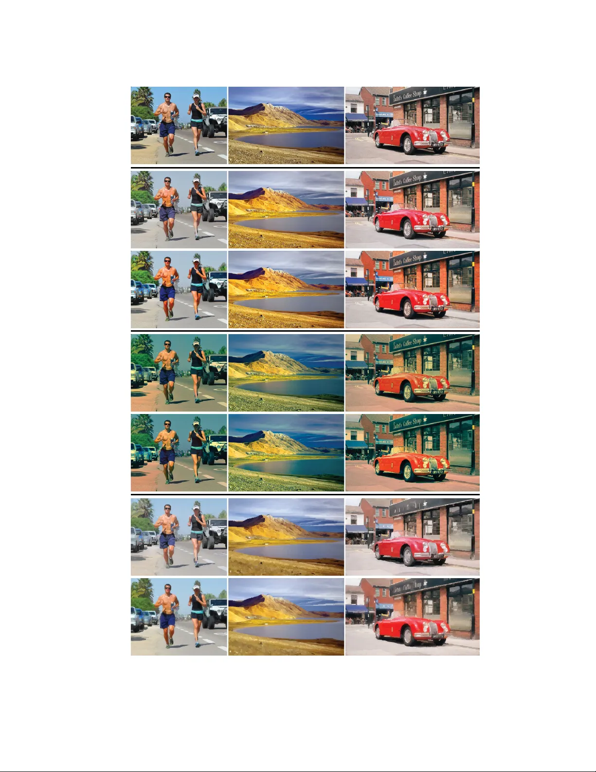
A utomatic Photo Adjustment Using Deep Neural Netw or ks Zhicheng Y an University of Illinois at Urbana Champaign Hao Zhang † Carnegie Mellon University Bao yuan Wang Microsoft Research Sylvain P aris Adobe Research Yizhou Y u The University of Hong K ong and Univ ersity of Illinois at Urbana Champaign Photo retouching enables photographers to in voke dramatic visual impres- sions by artistically enhancing their photos through stylistic color and tone adjustments. Howe ver , it is also a time-consuming and challenging task that requires advanced skills be yond the abilities of casual photographers. Using an automated algorithm is an appealing alternative to manual w ork but such an algorithm faces man y hurdles. Many photographic styles rely on subtle adjustments that depend on the image content and ev en its semantics. Further , these adjustments are often spatially v arying. Because of these characteris- tics, existing automatic algorithms are still limited and cov er only a subset of these challenges. Recently , deep machine learning has shown unique abilities to address hard problems that resisted machine algorithms for long. This motiv ated us to explore the use of deep learning in the context of photo editing. In this paper, we explain how to formulate the automatic photo adjustment problem in a way suitable for this approach. W e also introduce an image descriptor that accounts for the local semantics of an image. Our experiments demonstrate that our deep learning formulation applied using these descriptors successfully capture sophisticated photographic styles. In particular and unlike previous techniques, it can model local adjustments that depend on the image semantics. W e sho w on sev eral examples that this yields results that are qualitatively and quantitatively better than previous work. Categories and Subject Descriptors: I.4.3 [ Image Processing and Com- puter Vision ]: Enhancement; I.4.10 [ Image Processing and Computer V ision ]: Representation— Statistical Authors’ email addresses: zyan3@illinois.edu, hao@cs.cmu.edu, baoyuanw@microsoft.com, sparis@adobe.com, yizhouy@acm.org. † This work was conducted when Hao Zhang was an intern at Microsoft Research. Permission to make digital or hard copies of part or all of this work for personal or classroom use is granted without fee pro vided that copies are not made or distributed for profit or commercial advantage and that copies show this notice on the first page or initial screen of a display along with the full citation. Copyrights for components of this work o wned by others than A CM must be honored. Abstracting with credit is permitted. T o copy otherwise, to republish, to post on servers, to redistribute to lists, or to use any component of this work in other works requires prior specific permission and /or a fee. Permissions may be requested from Publications Dept., A CM, Inc., 2 Penn Plaza, Suite 701, New Y ork, NY 10121-0701 USA, fax + 1 (212) 869-0481, or permissions@acm.org. c  YYYY A CM 0730-0301/YYYY/15-AR TXXX $10.00 DOI 10.1145/XXXXXXX.YYYYYYY http://doi.acm.org/10.1145/XXXXXXX.YYYYYYY Additional Ke y W ords and Phrases: Color Transforms, Feature Descriptors, Neural Networks, Photo Enhancement 1. INTRODUCTION W ith the prev alence of digital imaging de vices and social network- ing, sharing photos through social media has become quite popular . A common practice in this type of photo sharing is artistic enhance- ment of photos by various Apps such as Instagram. In general, such photo enhancement is artistic because it not only tries to correct photographic defects (under/ov er exposure, poor contrast, etc.) b ut also aims to in voke dramatic visual impressions by stylistic or ev en exaggerated color and tone adjustments. T raditionally , high-quality enhancement is usually hand-crafted by a well-trained artist through extensi ve labor . In this work, we study the problem of learning artistic photo enhancement styles from image exemplars. Specifically , gi ven a set of image pairs, each representing a photo before and after pix el-level tone and color enhancement following a particular style, we wish to learn a computational model so that for a novel input photo we can apply the learned model to automatically enhance the photo following the same style. Learning a high-quality artistic photo enhancement style is chal- lenging for sev eral reasons. First, photo adjustment is often a highly empirical and perceptual process that relates the pixel colors in an enhanced image to the information embedded in the original image in a complicated manner . Learning an enhancement style needs to extract an accurate quantitativ e relationship underlying this process. This quantitati ve relationship is likely to be complex and highly nonlinear especially when the enhancement style re- quires spatially varying local adjustments. It is nontrivial to learn a computational model capable of representing such a complicated relationship accurately , and lar ge-scale training data is likely to be necessary . Therefore, we seek a learning model scalable with re- spect to both the feature dimension and data size and efficiently computable with high-dimensional, large-scale data. Second, an artistic enhancement is typically semantics-aware. An artist does not see indi vidual pixels; instead he/she sees semantically meaningful objects (humans, cars, animals, etc.) and determines the type of adjustments to improve the appearance of the objects. F or example, it is likely that an artist pays more attention to improve the appearance of a human figure than a region of sky in the same ACM T ransactions on Graphics, V ol. VV , No. N, Article XXX, Publication date: Month YYYY . 2 • Z. Y an, H. Zhang, B. Wang, S. Paris, and Y . Y u (a) (b) (c) Fig. 1. An example of our semantics-a ware photo enhancement style, which extends the “cross processing” ef fect in a local manner . Left : input image; Middle : enhanced image by our deep learning based automatic approach; Right : groundtruth image manually enhanced by a photographer, who applied different adjustment parameters in different semantic re gions. See more results of such effects in Section 7.1 and the supplemental materials. photo. W e would like to incorporate this semantics-awareness in our learning problem. One challenge is the representation of semant ic information in learning so that the learned model can perform image adjustments according to the specific content as human artists do. W e present an automatic photo enhancement method based on deep machine learning. This approach has recently accumulated impressiv e successes in domains such as computer vision and speech analysis for which the semantics of the data plays a major role, e.g., [V incent et al . 2008; Krizhevsk y et al . 2012]. This moti vated us to explore the use of this class of techniques in our context. T o address the challenges mentioned above, we cast ex emplar-based photo adjustment as a regression problem, and use a Deep Neural Network (DNN) with multiple hidden layers to represent the highly nonlinear and spatially varying color mapping between input and enhanced images. A deep neural network (DNN) is a uni versal approximator that can represent arbitrarily complex continuous functions [Hornik et al . 1989]. It is also a compact model which is readily scalable with respect to high-dimensional, large-scale data. Feature design is a key issue that can significantly af fect the ef fec- tiv eness of DNN. T o make sure the learned color mapping responds to complex color and semantic information, we design informati ve yet discriminati ve feature descriptors that serve as the input to the DNN. For each input image pix el, its feature descriptor consists of three components, which reflect respecti vely the statistical or seman- tic information at the pixel, conte xtual, and global le vels. The global feature descriptor is based on global image statistics, whereas the context feature descriptor is based on semantic information extracted from a large neighborhood around the pix el. Understanding image semantics has been made possible with recent advances in scene understanding and object detection. W e use existing algorithms to annotate all input image pixels and the semantics information from the annotated images are incorporated into a nov el context feature descriptor . Contributions . In summary , our proposed photo enhancement technique has the following contrib utions. — It introduces the first automatic photo adjustment framew ork based on deep neural networks. A v ariety of normal and artistic photo enhancement styles can be achie ved by training a distinct model for each enhancement style. The quality of our results is superior to that of existing methods. — Our framew ork adopts informative yet discriminati ve image fea- ture descriptors at the pixel, contextual and global lev els. Our context descriptor exploits semantic analysis o ver multiscale spa- tial pooling regions. It has achie ved improv ed performance over a single pooling region. — Our method also includes an ef fectiv e algorithm for choosing a representativ e subset of photos from a lar ge collection so that a photo enhancement model trained ov er the chosen subset can still produce high-quality results on nov el testing images. While a contribution of our w ork is the application of deep ma- chine learning in a ne w context, we use a standard learning proce- dure and do not claim any contribution in the design of the learning algorithm itself. Similarly , while we propose a possible design for semantic context descriptor , and demonstrate its effecti veness, a comprehensiv e exploration of the design space for such descriptors is beyond the scope of this paper . Complete source codes and datasets used by our system are pub- licly av ailable on Github 1 . 2. RELA TED WORK T raditional image enhancement rules are primarily determined em- pirically . There are many software tools to perform fully automatic color correction and tone adjustment, such as Adobe Photoshop, Google Auto A wesome, and Microsoft Office Picture Manager . In addition to these tools, there exists much research on either interac- tiv e [Lischinski et al . 2006; An and Pellacini 2008] or automatic [Bae et al . 2006; Cohen-Or et al . 2006] color and tone adjustment. Automatic methods typically operate on the entire image in a global manner without taking image content into consideration. T o address this issue, Kaufman et al. [2012] introduces an automatic method that first detects semantic content, including faces, sky as well as shadowed salient regions, and then applies a sequence of empiri- cally determined steps for saturation, contrast as well as exposure adjustment. Howe ver , the limit of this approach is that output style is hard-coded in the algorithm and cannot be easily tuned to achiev e a desired style. In comparison and as we shall see, our data-dri ven approach can easily be trained to produce a variety of styles. Further , these techniques rely on a fixed pipeline that is inherently limited in its ability to achie ve user-preferred artistic enhancement ef fects, especially the exaggerated and dramatic ones. In practice, a fixed- pipeline technique works well for a certain class of adjustments and only produces approximate results for effects outside this class. For instance, Bae et al. [2006] do well with tonal global transforms but 1 https://github .com/stephenyan1984/dl-image-enhance https://github .com/stephenyan1984/cuda convnet plus A CM T ransactions on Graphics, V ol. VV , No. N, Article XXX, Publication date: Month YYYY . A utomatic Photo Adjustment Using Deep Neural Networks • 3 do not model local edits, and Kaufman et al. [2012] perform well on a predetermined set of semantic categories b ut does not handle elements outside this set. In comparison, deep learning provides a univ ersal approximator that is trained on a per-style basis, which is key to the success of our approach. Another line of research for photo adjustment is primarily data- driv en. Learning based image enhancement [Kang et al . 2010; Joshi et al . 2010; Caicedo et al . 2011; Bychkovsk y et al . 2011] and image restoration [Dale et al . 2009] have shown promising results and therefore receiv ed much attention. Kang et al. [2010] found that image quality assessment is actually v ery much personalized, which results in an automatic method for learning individual preferences in global photo adjustment. Bychko vsky et al. [2011] introduces a method based on Gaussian processes for learning tone mappings according to global image statistics. Since these methods were de- signed for global image adjustment, they do not consider local image contexts and cannot produce spatially v arying local enhancements. W ang et al. [2011] proposes a method based on piecewise approxi- mation for learning color mapping functions from ex emplars. It does not consider semantic or contextual information either . In addition, it is not fully automatic, and relies on interactiv e soft segmentation. It is infeasible for this technique to automatically enhance a collection of images. In comparison, this paper proposes a scalable framework for learning user-defined comple x enhancement effects from e xem- plars. It explicitly performs generic image semantic analysis, and its image enhancement models are trained using feature descriptors constructed from semantic analysis results. Hwang et al. [2012] proposes a context-aware local image en- hancement technique. This technique first searches for the most similar images and then the most similar pixels within them, and finally apply a combination of the enhancement parameters at the most similar pixels to the considered pixel in the new test image. W ith a sufficiently large image database, this method works well. But in practice, nearest-neighbor search requires a fairly large train- ing set that is challenging to create and slow to search, thereby limiting the scalability of this approach. Another dif ference with our approach is that, to locate the most similar pixels, this method uses low- and mid-lev el features (i.e., color and SIFT) whereas we also consider high-lev el semantics. W e shall see in the result section that these dif ferences hav e a significant impact on the adjustment quality in sev eral cases. 3. A DEEP LEARNING MODEL Let us no w discuss ho w we cast ex emplar-based photo adjustment as a regression problem, and how we set up a DNN to solve this regression problem. A photo enhancement style is represented by a set of exemplar image pairs Λ = { I k , J k } m k =1 , where I k and J k are respectiv ely the images before and after enhancement. Our premise is that there exists an intrinsic color mapping function F that maps each pixel’ s color in I k to its corresponding pixel’ s color in J k for every k . Our goal is to train an approximate function ˜ F using Λ so that ˜ F may be applied to new images to enhance the same style there. For a pixel p i in image I k , the value of ˜ F is simply the color of image J k at pixel p i , whereas the input of ˜ F is more complex because ˜ F depends on not only the color of p i in I k but also additional local and global information extracted from I k , thus we formulate ˜ F as a parametric function ˜ F (Θ , x i ) , where Θ represents the parameters and x i represents the feature vector at p i that encompasses the color of p i in I k as well as additional local and global information. W ith this formulation, training the function . . . . . . . . . b ia s b ia s b ia s . . . O u t p u t L a y er : Φ ( Θ , X i ) Hi d d en L a y er Hi d d en L a y er In p u t L a y e r L 2 i a 2 i 1 . . . C o s t l a y er Q u a d r a t i c b a s i s : V ( c i ) Fig. 2. The architecture of our DNN. The neurons above the dash line indicate how we compute the cost function in (3). Note that the weights for the connections between the blue neurons and the yellow neurons are just the elements of the quadratic color basis, and the activation function in the yellow and purple neurons is the identity function. During training, error backpropagation starts from the output layer , as the connection weights above the dash line ha ve already been fixed. ˜ F using Λ becomes computing the parameters Θ from training data Λ through nonlinear regression. High-frequency pix elwise color variations are dif ficult to model because they force us to choose a mapping function which is sen- sitiv e to high-frequency details. Such a mapping function often leads to noisy results in relatively smooth regions. T o tackle this problem we use a color basis vector V ( c i ) at pixel p i to rewrite ˜ F as ˜ F = Φ(Θ , x i ) V ( c i ) , which expresses the mapped color, ˜ F , as the result of applying the color transform matrix Φ(Θ , x i ) to the color basis vector V ( c i ) . V ( c i ) is a vector function taking different forms when it works with different types of color transforms. In this paper we work in the CIE Lab color space, and the color at p i is c i = [ L i a i b i ] T and V ( c i ) = [ L i a i b i 1] T if we use 3x4 affine color transforms. If we use 3x10 quadratic color transforms, then V ( c i ) = [ L 2 i a 2 i b 2 i L i a i L i b i a i b i L i a i b i 1] . Since the per-pix el color basis vector V ( c i ) varies at similar frequencies as pixel colors, it can absorb much high-frequency color v ariation. By factorizing out the color variation associated with V ( c i ) , we can let Φ(Θ , x i ) focus on modeling the spatially smooth but otherwise highly nonlinear part of ˜ F . W e learn Φ(Θ , x i ) by solving the following least squares min- imization problem defined over all training pixels sampled from Λ : arg min Φ ∈H n X i k Φ(Θ , x i ) V ( c i ) − y i k 2 , (1) where H represents the function space of Φ(Θ , x i ) and n is the total number of training pixels. In this paper , we represent Φ(Θ , x i ) as a DNN with multiple hidden layers. A CM T ransactions on Graphics, V ol. VV , No. N, Article XXX, Publication date: Month YYYY . 4 • Z. Y an, H. Zhang, B. Wang, S. Paris, and Y . Y u L a b Input image Visualization of 3 x 10 coecients of the quadratic color transf orm Fig. 3. (Left) Input image, and (Right) visualization of its per-pixel quadratic color transforms, Φ(Θ , x i ) , each of which is a 3 × 10 matrix. Each image on the right visualizes one coefficient in this matrix at all pixel locations. Coefficients are linearly mapped to [0,1] in each visualization image for better contrast. This visualization illustrates two properties of the quadratic color transforms: 1) they are spatially varying and 2) they are smooth with much high-frequenc y content suppressed. 3.1 Neural Network Architecture and T raining Our neural network follows a standard architecture that we describe below for the sak e of completeness. Multi-layer deep neural networks have pro ven to be able to repre- sent arbitrarily complex continuous functions [Hornik et al . 1989]. Each network is an ac yclic graph, each node of which is a neuron. Neurons are organized in a number of layers, including an input layer , one or more hidden layers, and an output layer . The input layer directly maps to the input feature vector , i.e. x i in our prob- lem. The output layer maps to the elements of the color transform, Φ(Θ , x ν ) . Each neuron within a hidden layer or the output layer takes as input the responses from all the neurons in the preceding layer . Each connection between a pair of neurons is associated with a weight. Let us denote v l j as the output of the j -th neuron in the l -th layer . Then v l j is expressed as follo ws: v l j = g w l j 0 + X k> 0 w l j k v l − 1 k ! (2) where w l j k is the weight associated with the connection between the j -th neuron in the l -layer and the k -th neuron in the ( l − 1) -th layer , and g ( z ) is an activ ation function which is typically nonlin- ear . W e choose the rectified linear unit (ReLU) [Krizhevsky et al . 2012], g ( z ) = max(0 , z ) , as the activ ation function in our net- works. Compared with other widely used acti vation functions, such as the hyperbolic tangent, g ( z ) = tanh( z ) = 2 / (1 + e − 2 z ) − 1 , or the sigmoid, h ( x ) = (1 + e − x ) − 1 , ReLU has a fe w advantages, including inducing sparsity in the hidden units and accelerating the con vergence of the training process. Note that there is no nonlinear activ ation function for neurons in the output layer . The output of a neuron in the output layer is only a linear combination of its inputs from the preceding layer . Figure 2 shows the overall architecture, which has two e xtra layers (yellow and purple neurons) abov e the output layer for computing the product between the color transform and the color basis v ector . Giv en a neural network architecture for color mapping, H in (1) should be the function space spanned by all neural networks with the same architecture b ut different weight parameters Θ . Once the network architecture has been fix ed, gi ven a train- ing dataset, we use the classic error backpropagation algorithm to train the weights. In addition, we apply the Dr opout training strategy [Krizhevsk y et al . 2012; Hinton et al . 2012], which has been shown v ery useful for improving the generalization capability . Fig. 4. Our multiscale spatial pooling schema. In each pooling region, we compute a histogram of semantic categories. The shown three-scale scheme has 9*2+1=19 pooling regions. In our experiments, we use a four-scale scheme with 28 pooling regions. W e set the output of each neuron in the hidden layers to zero with probability 0.5. Those neurons that have been “dropped out” in this way do not contrib ute to the forward pass and do not participate in error backpropagation. Our experiments sho w that adding Dropout during training typically reduces the relativ e prediction error on testing data by 2 . 1% , which actually makes a significant difference in the visual quality of the enhanced results. Figure 3 visualizes the per-pix el quadratic color transforms, Φ(Θ , x i ) , generated by a trained DNN for one example image. W e can see that the learned color mappings are smooth in most of the local regions. 4. FEA TURE DESCRIPTORS Our feature descriptor ( x i ) at a sample pixel p i serves as the in- put layer in the neural network. It has three components, x i = ( x p i , x c i , x g i ) , where x p i represents pixelwise features, x c i represents contextual features computed for a local region surrounding p i , and x g i represents global features computed for the entire image where p i belongs. The details about these three components follow . 4.1 Pix elwise Features Pixelwise features reflect high-resolution pixel-lev el image varia- tions, and are indispensable for learning spatially varying photo A CM T ransactions on Graphics, V ol. VV , No. N, Article XXX, Publication date: Month YYYY . A utomatic Photo Adjustment Using Deep Neural Networks • 5 -1 - 0 . 5 0 0 . 5 1 -1 - 0 . 5 0 0 . 5 1 u n k n o w n b u i l d i n g c a r g r a s s p e r s o n r o a d t r e e Input Image Parsing Map Car Detection Person Detection Final Label Map Fig. 5. Pipeline for constructing our semantic label map. Starting with an input image, we first perform scene parsing to obtain a parsing map, then we run object detectors to obtain a detection map for each object category (i.e, car , person), finally we superpose the detection maps onto the parsing map to obtain the final semantic label map (the rightmost image). enhancement models. They are defined as x p i = ( c i , p i ) , where c i represents the av erage color in the CIELab color space within the 3x3 neighborhood, and p i = ( x i , y i ) denotes the normalized sample position within the image. 4.2 Global F eatures In photographic practice, global attributes and ov erall impressions, such as the average intensity of an image, at least have partial in- fluence on artists when the y decide how to enhance an image. W e therefore incorporate global image features in our feature represen- tation. Specifically , we adopt six types of global features proposed in [Bychkovsk y et al . 2011], including intensity distribution, scene brightness, equalization curves, detail-weighted equalization curves, highlight clipping, and spatial distribution , which altogether giv e rise to a 207-dimensional vector . 4.3 Conte xtual Features Our contextual features try to characterize the distribution of se- mantic categories, such as sky , building, car, person, and tree, in an image. Such features are extracted from semantic analysis re- sults within a local region surrounding the sample pixel. T ypical image semantic analysis algorithms include scene parsing [T ighe and Lazebnik 2010; Liu et al . 2011] and object detection [V iola and Jones 2001; Felzenszwalb et al . 2008; W ang et al . 2013]. Scene pars- ing tries to label ev ery pixel in an image with its semantic category . Object detection on the other hand trains one highly specialized detector for ev ery category of objects (such as dogs). Scene parsing is good at labeling categories (such as grass, roads, and sky) that hav e no characteristic shape but relati vely consistent texture. These categories ha ve a large scale, and typically form the background of an image. Object detectors are better at locating categories (such as persons and cars), which are better characterized by their overall shape than local appearance. These categories hav e a smaller scale, and typically occup y the fore ground of an image. Because these two types of techniques are complementary to each other , we perform semantic analysis using a combination of scene parsing and object detection algorithms. Figure 5 illustrates one fusion example of the scene parsing and detection results. W e use existing algorithms to automatically annotate all input image pixels and the semantics information from the annotated images are gathered into a nov el context feature descriptor . During pixel annotation, we perform scene parsing using the state-of-the- art algorithm in [T ighe and Lazebnik 2010]. The set of semantic categories, S p , during scene parsing include such object types as sky , road, river , field and grass. . After the scene parsing step, we obtain a parsing map, denoted as I p , each pixel of which recei ves one category label from S p , indicating that with a high probability , the corresponding pixel in the input image is covered by a semantic instance in that cate gory . W e further apply the state-of-the-art object detector in [W ang et al . 2013] to detect the pixels cov ered by a predefined set of foreground object types, O d , which include person, train, bus and building. After the detection step, we obtain one confidence map for each predefined type. W e fuse all confidence maps into one by choosing, at e very pixel, the object label that has the highest confidence v alue. This fused detection map is denoted as I d . W e further mer ge I d with I p so that those pixel labels from I d with confidence larger than a predefined threshold are used to ov erwrite the corresponding labels from I p . Since scene parsing and object detection results tend to be noisy , we rely on voting and automatic image segmentation to perform label cleanup in the merged label map. W ithin each image segment, we reset the label at ev ery pixel to the one that appears most frequently in the segment. In our experiments, we adopt the image segmentation algorithm in [Arbelaez et al . 2011]. This cleaned map becomes our final semantic label map, I label . Giv en the final semantic label map for the entire input image, we construct a contextual feature descriptor for each sample pixel to represent multiscale object distrib utions in its surroundings. For a sample point p i , we first define a series of nested square regions, { R 0 , R 1 , . . . , R τ } , all centered at p i . The edge length of these re- gions follows a geometric series, i.e. λ k = 3 λ k − 1 ( k = 1 , . . . , τ ) , making our feature representation more sensitiv e to the semantic contents at nearby locations than those farther a way . W e further sub- divide the ring between e very two consecuti ve squares, R k +1 − R k , into eight rectangles, as shown in Figure 4. Thus, we end up with a total of 9 τ + 1 regions, including both the original regions in the series as well as re gions generated by subdi vision. For each of these regions, we compute a semantic label histogram, where the number of bins is equal to the total number of semantic cate gories, N = |S p S O d | . Note that the histogram for R k is the sum of the histograms for the nine smaller regions within R k . Such spatial pooling can make our feature representation more robust and better tolerate local geometric deformations. The final conte xtual feature descriptor at p i is defined to be the concatenation of all these seman- tic label histograms. Our multiscale context descriptor is partially inspired by shape contexts [Belongie et al . 2002]. Howe ver , unlike the shape context descriptor , our regions and subre gions are either rectangles or squares, which f acilitate fast histogram computation based on integral images (originally called summed area tables) [V i- ola and Jones 2001]. In practice, we pre-compute N integral images, one for each semantic cate gory . Then the value of each histogram bin can be calculated within constant time, which is extremely fast compared with the computation of shape contexts. T o the best of our knowledge, our method is the first one that explicitly constructs se- mantically meaningful contextual descriptors for learning complex image enhancement models. It is important to verify whether the complexity of our contextual features is necessary in learning complex spatially varying local adjustment effects. W e have compared our results against those A CM T ransactions on Graphics, V ol. VV , No. N, Article XXX, Publication date: Month YYYY . 6 • Z. Y an, H. Zhang, B. Wang, S. Paris, and Y . Y u obtained without contextual features as well as those obtained from simpler contextual features based on just one pooling region (vs. our 28 multiscale regions) at the same size as our largest region. From Figure 11, we can see that our contextual features are able to produce local adjustment results closest to the ground truth. Discussion . The addition of this semantic component into our fea- ture vectors is a major dif ference with previous work. As sho wn in Figure 11 and in the result section, the design that we propose for this component is effecti ve and produces a significant improvement in practice. That said, we acknowledge that other options may be possible and we believ e that exploring the design space of semantic descriptors is an exciting a venue for future work. 5. TRAINING D A T A SAMPLING AND SELECTION 5.1 Super pix el Based Sampling When training a mapping function using a set of images, we prefer not to make use of all the pixels as such a dense sampling would result in unbalanced training data. For e xample, we could have too many pixels from large “sky” regions while relati vely few from smaller “person” regions, which could e ventually result in a serious bias in the trained mapping function. In addition, an overly dense sampling unnecessarily increases the training cost, as we need to handle millions of pixel samples. Therefore, we apply a superpixel based method to collect training samples. For each training image I , we first apply the graph-based se gmentation [Felzenszwalb and Huttenlocher 2004] to divide the image into small homogeneous yet irregularly shaped patches, each of which is called a superpixel. Note that a superpixel in a smooth region may be larger than one in a region with more high-frequency details. W e require that the color transform returned by our mapping function at the centroid of a superpixel be used for predicting with sufficient accuracy the adjusted color of all pixels within the same superpix el. T o av oid bias, we randomly sample a fixed number of pixels from e very superpix el. Let ν be any superpixel from the original images (before adjustment) in Λ , and S ν be the set of pixels sampled from ν . W e re vise the cost function in (1) as follo ws to reflect our superpixel-based sampling and local smoothness requirement. X ν X j ∈ S ν k Φ(Θ , x ν ) V ( c j ) − y j k 2 , (3) where Θ represents the set of trained weights in the neural network, x ν is the feature vector constructed at the pixel closest to the centroid of ν , V ( c j ) denotes the color basis vector of a sample pix el within ν , and y j denotes the adjusted color of the same sample within ν . 5.2 Cross-Entrop y Based Image Selection In example-based photo enhancement, example images that demon- strate a certain enhancement style often need to be manually pre- pared by human artists. It is a labor intensive task to adjust many images as each image has multiple attributes and regions that can be adjusted. Therefore, it is much desired to pre-select a small number of representativ e training images to reduce the amount of human work required. On the other hand, to make a learned model achie ve a strong prediction capability , it is necessary for the selected training images to hav e a reasonable coverage of the feature space. In this section, we introduce a cross-entropy based scheme for selecting a subset of representativ e training images from a large collection. W e first learn a codebook of feature descriptors with K = 400 codew ords by running K-means clustering on feature descriptors collected from all training images. Then e very original Algorithm 1: Small Training Set Selection Input : A large image collection, Ω I ; The desired number of representativ e images, m d Output : A subset Ω with m d images selected from Ω I 1 Initialize Ω ← ∅ 2 for i = 1 to m d do 3 I ∗ = arg max I ∈ Ω I − Ω − P j H Ω 0 ( j ) log H Ω 0 ( j ) , 4 where Ω 0 = Ω ∪ { I } ; 5 Ω = Ω ∪ { I ∗ } 6 end feature descriptor can find its closest codeword in the codebook via vector quantization, and each image can be viewed as “a bag of” codew ords by quantizing all the feature descriptors in the image. W e further b uild a histogram for ev ery image using the codew ords in the codebook as histogram bins. The v alue in a histogram bin is equal to the number of times the corresponding code word appears in the image. Let H k be the histogram for image I k . For an y sub- set of images Ω from an initial image collection Ω I , we compute the accumulated histogram H Ω by simply performing elementwise summation ov er the individual histograms of the images in Ω . W e further evaluate the representative power of Ω using the cross en- tropy of H Ω . That is, Entropy ( H Ω ) = − P j H Ω ( j ) log H Ω ( j ) , where H Ω ( j ) denotes the j -th element of H Ω . A large cross en- tropy implies that the codewords corresponding to the histogram bins are ev enly distributed in the images in Ω and vice versa. Thus, to encourage an even coverage of the feature space, the set of se- lected images essentially need to be the solution of the following expensi ve combinatorial optimization, Ω = arg max Ω ∈ Ω I − X j H Ω ( j ) log H Ω ( j ) . (4) In practice, we seek an approximate solution by progressi vely adding one image to Ω ev ery time until we ha ve a desired number of images in the subset. Every time the added image maximizes the cross en- tropy of the e xpanded subset. This process is illustrated in Algorithm 1. 6. O VER VIEW OF EXPERIMENTS Our proposed method is well suited for learning comple x and highly nonlinear photo enhancement styles, especially when the style re- quires challenging spatially varying local enhancements. Successful local enhancement may not only rely on the content in a specific local region, b ut also contents in its surrounding areas. In that sense, such operations could easily result in comple x effects that require stylistic or ev en exaggerated color transforms, making previous global methods (e.g., [Bychkovsky et al . 2011]) and local empirical methods (e.g., [Kaufman et al . 2012]) inapplicable. In contrast, our method was designed to address such challenges with the help of powerful conte xtual features and the strong regression capability of deep neural networks. T o fully e valuate our method, we hired one professional photog- rapher who carefully retouched three different stylistic local effects using hundreds of photos. Section 7 reports experiments we hav e conducted to ev aluate the performance of our method. Although our technique was designed to learn complex local effects, it can be readily applied to global image adjustments without any dif ficulty . Experiments in Section 8 and the supplemental materials show that our technique achiev es superior performance both visually and nu- A CM T ransactions on Graphics, V ol. VV , No. N, Article XXX, Publication date: Month YYYY . A utomatic Photo Adjustment Using Deep Neural Networks • 7 merically when compared with other state-of-the-art methods on the MIT -Adobe Fivek dataset. T o objectively e valuate the ef fectiveness of our method, we have further conducted two user studies (Section 8.3) and obtained very positi ve results. 6.1 Experimental Setup Neural Network Setup . Throughout all the experiments in this paper , we use a fixed DNN with one input layer, tw o hidden layers, and one output layer (Figure 2). The number of neurons in the hidden layers were set empirically to 192, and the number of neurons in the output layer were set equal to the number of coef ficients in the predicted color transform. Our experiments have confirmed that quadratic color transforms can more faithfully reproduce the colors in adjusted images than affine color transforms. Therefore, there are 30 neurons in the output layer , 10 for each of the three color channels. Data Sampling . Since we learn pix el-level color mappings, every pixel within the image is a potential training sample. In practice, we segment each image into around 7,000 superpixels, from each of which we randomly select 10 pix els. Therefore, for example, e ven if we only have 70 example image pairs for learning one specific local effect, the number of training samples can be as large as 4.9 million. Such a large-scale training set can largely eliminate the risk of overfitting. It typically takes a few hours to finish training the neural network on a medium size training dataset with hundreds of images. Nev ertheless, a trained neural network only needs 0.4 second to enhance a 512-pixel wide test image. Image Enhancement with Learned Color Mappings . Once we hav e learned the parameters (weights) of the neural network, during the image enhancement stage, we apply the same feature extraction pipeline to an input image as in the training stage. That is, we first perform scene parsing and object detection, and then apply graph-based segmentation to obtain superpixels. Lik ewise, we also extract a feature v ector at the centroid of every superpixel, and apply the color transform returned by the neural network to every pixel within the superpixel. Specifically , the adjusted color at pixel p i is computed as y i = Φ(Θ , x ν i ) V ( c i ) , where ν i is the superpixel that cov ers p i . 7. LEARNING LOCAL ADJUSTMENTS 7.1 Three Stylistic Local Eff ects W e manually do wnloaded 115 images from Flickr and resized them such that their larger dimension has 512 pixels. 70 images were chosen for training and the remaining 45 images for testing. A pro- fessional photographer used Photoshop to retouch these 115 images and produce the datasets for three different stylistic local effects. She could perform a wide range of operations to adjust the images, including selecting local objects/areas with the region selection tool, creating layers with layer masks, blending different layers using various modes, just to name a few . T o reduce subjective variation during retouching, she used the “actions” tool, which records a se- quence of operations, which can be repeatedly applied to selected image regions. The first local ef fect ” For eground Pop-Out ” was created by in- creasing both the contrast and color saturation of foreground salient objects/regions, while decreasing the color saturation of the back- ground. Before performing these operations, foreground salient regions need to be interacti vely segmented out using region selec- tion tools in Photoshop. Such segmented regions were only used for dataset production, and they are not used in our enhancement pipeline. This local ef fect makes foreground objects more visually vivid while making the background less distractiv e. Figure 6 (b) and (c) show three e xamples of our automatically enhanced results and groundtruth results from the photographer. Refer to the supplemen- tal materials for the training data as well as our enhanced testing photos. Our second effect ” Local Xpro ” was created by generalizing the popular ”cross processing” effect in a local manner . Within Pho- toshop, the photographer first predefined multiple ”Profiles”, each of which is specifically tailored for one of the semantic categories used in scene parsing and object detection in section 4.3. All the profiles share a common series of operations, such as the adjustment of indi vidual color channels, color blending across color channels, hue/saturation adjustment as well as brightness/contrast manipula- tion, just to name a few . Nonetheless, each profile defines a distinct set of adjustment parameters tailored for its corresponding category . When retouching a photo, the photographer used region selection tools to isolate image regions and then applied one suitable profile to each image region according to the specific semantic content within that region. T o av oid artifacts along region boundaries, she could also slightly adjust the color/tone of local regions after the application of profiles. Although the profiles roughly follow the ”cross processing” style, the choice of local profiles and additional minor image editing were heavily influenced by the photographer’ s personal taste which can be naturally learned through exemplars. Figure 6 (d)&(e) show three e xamples in this effect, and compare our enhanced results against groundtruth results. Figure 1 shows another example of this ef fect. T o further increase di versity and complexity , we asked the pho- tographer to create a third local effect ” W atercolor ”, which tries to mimic certain aspects of the ”watercolor” painting style. For exam- ple, watercolors tend to be brighter with lower saturation. W ithin a single brush region, the color variation also tends to be limited. The photographer first applied similar operations as in the Fore- ground Pop-Out effect to the input images, including increasing both contrast and saturation of foreground regions as well as de- creasing those of background regions. In addition, the brightness of both foreground and background regions are increased by dif ferent amounts. She further created two layers of brush effects from the same brightened image, using lar ger “brushes” on one layer and a smaller one on the other . On the first layer , the brush size for the foreground and the background are also different. Finally , these two layers are composited together using the ’Lighten’ mode in Pho- toshop. Overall, this effect results in highly comple x and spatially varying color transforms, which force the neural network to heavily rely on local contextual features during re gression. Figure 6 (f)&(g) show the enhanced results of three testing exam- ples and their corresponding groundtruth results. T o simulate brush strokes, after applying the same color transform to all pixels in a superpixel, we calculate the av erage color within the superpixel and fill the superpixel with it. See another example of W atercolor effect as well as visualized superpixels in Fig 7. Our automatic results look visually similar to the ones produced by the photographer. Refer to the supplemental materials for more examples enhanced with this effect. Note that our intention here is not rigorously simulating watercolors, but e xperimentally validating that our technique is able to accurately learn such complex local adjustments. T o successfully learn an enhancement effect, it is important to make the adjustments on individual training images consistent. In practice, we have found the following strategies are helpful in in- creasing such consistency across an image set. First, as artistic adjustment of an image in volves the personal taste of the photogra- pher , the result could be quite dif ferent from different photographers. A CM T ransactions on Graphics, V ol. VV , No. N, Article XXX, Publication date: Month YYYY . 8 • Z. Y an, H. Zhang, B. Wang, S. Paris, and Y . Y u (a) (b) (c) (d) (e) (f ) (g) Fig. 6. Examples of three stylistic local enhancement effects. Row (a) : input images. Row (b)&(c) : our enhanced results and the groundtruth for the Fore ground Pop-Out effect. Row (d)&(e) : our enhanced results and the groundtruth for the Local Xpro ef fect. Row (f)&(g) : our enhanced results and the groundtruth for the W atercolor ef fect. A CM T ransactions on Graphics, V ol. VV , No. N, Article XXX, Publication date: Month YYYY . A utomatic Photo Adjustment Using Deep Neural Networks • 9 (a) (b) (c) (d) Fig. 7. An example of W atercolor local effect. (a) : input image. (b) : a visu- alization of superpixels used for simulating brush strokes. Each superpix el is filled with a random color . (c) : our enhanced result. (d) : the ground truth. Therefore, we al ways define a retouching style using photos adjusted by the same photographer . That means, ev en for the same input con- tent, retouched results by dif ferent photographers are always defined as dif ferent styles. Second, we inform the photographer the semantic object categories that our scene parsing and object detection algo- rithms are aware of. Consequently , she can apply similar adjustments to visual objects in the same semantic cate gory . Third, we use the ”actions” tool in Photoshop to faithfully record the ”Profiles” that should be applied to different semantic categories. This improves the consistency of color transforms applied to image regions with similar content and context. 7.2 Spatially V arying Color Mappings It is important to point out that the underlying color mappings in the local effect datasets are truly not global. They spatially vary within the image domain. T o verify this, we collect pixels from each semantic region of an image. By drawing scatter plots for different semantic regions using pixel color pairs from the input and retouched images, we are able to visualize the spatially varying color transforms. See such an example in Figure 9, which clearly shows that the color transforms differ in the sky , building, grass and road regions. Also, we can see that our method can successfully learn such spatially v arying complex color transforms. W e further conducted a comparison against [W ang et al . 2011], which adopts a local piecewise approximation approach. Howe ver , due to the lack of discriminativ e contextual features, their learned adjustment parameters tend to be similar across different re gions (Figure 8). 7.3 Generalization Capability Here we v erify the generalization capability of the DNN based photo adjustment models we trained using 70 image pairs. As mentioned earlier , the actual number of training samples f ar e xceeds the number of training image pairs because we use thousands of superpixels within each training image pair . As shown in Fig. 10, we apply our trained models to novel testing images with significant visual differences from any images in the training set. The visual objects in these images have either unique appearances or unique spatial configurations. T o illustrate this, we sho w the most similar training Fig. 8. Comparison with [W ang et al . 2011] on the Local Xpro effect. T op Left : Input image; T op Right : enhanced image by [W ang et al . 2011]; Bottom Left: enhanced image by our approach; Bottom Right: enhanced image by photographer . The enhanced image by our approach is closer to the ground truth generated by the photographer . images, which not only share the largest number of object and region categories with the testing image, but also have a content layout as similar as possible. In Fig 10 top, the mountain in the input image has an appearance and spatial layout that are different from the training images. In Fig 10 bottom, the appearances and spatial configuration of the car and people are also quite different from those of the training images. In despite of these differences, our trained DNN models are still able to adjust the input images in a plausible way . 7.4 Eff ectiveness of Contextual Features W e demonstrate the importance of contextual features in learning lo- cal adjustments in this subsection. First, we calculate the L 2 distance in the 3D CIELab color space between input images and ground truth produced by the photographer for all local effect datasets as shown in the second column of T able I. They numerically reflect the magnitude of adjustments the photographer made to the input images. Second, we numerically compare the testing errors of our enhanced results with and without the contextual feature in the third and fourth columns of T able I. Our experiments sho w that without contextual features, testing errors of our enhanced results tend to be relativ ely high. The mean L 2 error in the 3D CIELab color space reaches 9.27 , 9.51 and 9.61 respectiv ely for the Fore ground Pop-Out, Local Xpro and W atercolor ef fects. On the other hand, by including our proposed contextual feature, all errors drop significantly to 7.08 , 7.43 and 7.20 , indicating the necessity of such features. T able I. Statistics of three local effects and the mean L 2 testing errors. TE=T esting Error . Effect ground truth L 2 distance TE w/o context TE w/ con- text Foreground Pop-Out 13.86 9.27 7.08 Local Xpro 19.71 9.51 7.43 W atercolor 15.30 9.61 7.20 T o validate the effecti veness of our multiscale spatial pooling schema in our contextual feature design, we hav e experimented with A CM T ransactions on Graphics, V ol. VV , No. N, Article XXX, Publication date: Month YYYY . 10 • Z. Y an, H. Zhang, B. Wang, S. Paris, and Y . Y u b a L building grass b a L road sky Fig. 9. Scatter plots of color mappings. Middle (from top to bottom) : input image, semantic label map and the groundtruth for the Local Xpro effect. Left and right : color mapping scatter plots for four semantic regions. Each semantic region has three scatter plots corresponding to its L , a , b color channels. Each scatter plot visualizes two sets of points, which take the original v alue of a channel as the horizontal coordinate, and respectiv ely the predicted (red) and groundtruth (blue) adjusted values of that channel as the v ertical coordinate. Input Image W ithout Context Simple Context Our Context Ground T ruth Fig. 11. Ef fectiveness of our contextual features. Left: Input; Middle Left: enhanced without context; Middle: enhanced with simple contextual features (from a single pooling region); Middle Right: enhanced with our contextual features; Right: ground truth. It is obvious t hat among all enhanced results, the one enhanced using our contextual features is the closest to the ground truth. a simpler yet more intuiti ve conte xtual feature descriptor with just one pooling region (vs. our 28 multiscale re gions) at the same size as our largest re gion, and found that such simple contextual features are helpful in reducing the errors b ut not as effecti ve as ours. T aking the local W atercolor painting effect as an example, we observed the corresponding mean L 2 error is 8.28 , which drops from 9.61 , but still ob viously higher than our multiscale features 7.20 . This is because, with multiscale pooling regions, our features can achieve a certain de gree of translation and rotation inv ariance, which is crucial for the histogram based representation. W e have also performed visual comparisons. Fig. 11 shows one such example. W e can see that without our contextual feature, local regions in the enhanced photo might exhibit se vere color deviation from the ground truth. 7.5 Eff ectiveness of Lear ning Color T ransforms As sho wn in Figure 3, the use of color transforms helps absorb high- frequency color v ariations and enables DNN to regress the spatially smooth b ut otherwise highly nonlinear part of the color mapping. T o highlight the benefits of using color transforms, we train a different DNN to re gress the retouched colors directly . The DNN architecture is similar to the one described in section 6.1 except that there are only 3 neurons in the output layer, which represent the enhanced CIELab color . W e compare the testing L 2 errors on the Foregronud Pop-Out and Local Xpro datasets in T able II. On both datasets, the testing error increases by more than 20% which indicates the use of color transforms is beneficial in our task. 7.6 DNN Architecture The complexity of our DNN based model is primarily determined by the number of hidden layers and the number of neurons in each layer . Note that the complexity of the DNN architecture should meet the inherent comple xity of the learning task. If the DNN did not have the sufficient complexity to handle the gi ven task, the trained model would not ev en be able to accurately learn all the samples in the training set. On the other hand, if the complexity of the DNN exceeds the inherent complexity of the gi ven task, there exists the risk of overfitting and the trained model would not be able to generalize well on nov el testing data even though it could mak e the training error very small. The nature of the learning task in this paper is a regression prob- lem. It has been shown that a feedforward neural network with a single hidden layer [Hornik et al . 1989] can be used as a uni versal regressor and the necessary number of neurons in the hidden layer varies with the inherent complexity of the gi ven regression problem. In practice, howe ver , it is easier to achieve a small training error with a deeper network that has a relatively small number of neurons in the hidden layers. T o assess the impact of the design choices of T able II. Comparison of L 2 testing errors obtained from deep neural networks using and without using quadratic color transforms. Effect w/o transform w/ transform Foreground Pop-Out 8.90 7.08 Local Xpro 9.01 7.43 A CM T ransactions on Graphics, V ol. VV , No. N, Article XXX, Publication date: Month YYYY . A utomatic Photo Adjustment Using Deep Neural Networks • 11 (a) (b) (b) (c) (d) (a) (c) (d) Fig. 10. T wo examples of nov el image enhancement. T op : an example of the W atercolor effect. Bottom : an example of the Local Xpro effect. In each example, (a) : input image, (b) : our enhanced result, (c) : ground truth, (d) : training images most similar to the input image. Note that the input images in these examples hav e significant visual differences from any images in the training set. the DNN architecture, we ev aluate DNNs with a varying number of hidden layers and neurons. W e keep a held-out set of 30 images for validation and v ary the number of training images from 40 to 85 at a step size of 15 to ev aluate the impact of the size of the training set. W e repeat the e xperiments for five times with random training and testing partitions and report the averaged results. The F oreground Pop-Out dataset is used in this study . Fig 12 summarizes our experi- mental results. Overall, neural networks with a single hidden layer deliv er inferior performance than deeper networks. DNNs with 3 hidden layers do not perform as well as those with 2 hidden layers. For a DNN with 2 hidden layers, when the number of training im- ages exceeds 70, the testing error does not significantly improv e any more. In summary , DNNs with 2 hidden layers achie ve low testing errors and execute faster than those with 3 hidden layers in both training and testing stages. Therefore, we finally use a DNN with 2 hidden layers and 192 neurons each throughout this paper. 7.7 Comparison with Other Regression Methods Our DNN proves to be ef fectiv e for regressing spatially varying complex color transforms on the three local effect da tasets. It is also of great interest to ev aluate the performance of other regressors on our datasets. Specifically , we chose to compare DNN against two popular regression methods, Lasso [T ibshirani 1996] and random forest [Breiman 2001]. Both Lasso and random forest are scalable # of training images 40 55 70 85 Testing CIELab error 7 7.5 8 8.5 9 9.5 10 1 layers, 96 neurons 1 layers, 192 neurons 1 layers, 384 neurons 2 layers, 96 neurons 2 layers, 192 neurons 2 layers, 384 neurons 3 layers, 96 neurons 3 layers, 192 neurons 3 layers, 384 neurons Fig. 12. T esting error vs number of training images for DNNs of various architectures. Error bars are omitted for clarity . T able III. Comparison of L 2 testing errors obtained from different re gressors. Effect Lasso Random Forest DNN Foreground Pop-Out 11.44 9.05 8.90 Local Xpro 12.01 7.51 9.01 W atercolor 9.34 11.41 9.22 to the large number of training samples used in DNN training. W e use Lasso and a random forest to directly regress target CIELab colors using the same feature set as in DNN training, including pixelwise features, global features and contextual features. The hyperparameters of both Lasso and the random forest are tuned using cross validation. T o make a fair comparison, our DNN is also adapted to directly regress the tar get CIELab colors. A comparison of L 2 errors is summarized in T able III. The DNN significantly outperforms Lasso on the Foreground Pop-Out and Local Xpro datasets, and obtains slightly lower errors on the W atercolor dataset. Compared with the random forest, the DNN obtains lo wer testing errors on both Foreground Pop-Out and W atercolor datasets. On the Local Xpro dataset, the random forest obtains lo wer numerical errors than that of the DNN. Howe ver , after visual inspection, we found that colors generated by the random forest are not spatially smooth and blocky artifacts are prev alent in the enhanced images, as shown in Figure 13. This is because regression results from a random forest are based on values retrieved from various leaf nodes, and spatial smoothness of these retrie ved v alues cannot be guaranteed. In contrast, our trained DNN generates spatially smooth colors and does not giv e rise to such visual artifacts. 8. LEARNING GLOBAL ADJUSTMENTS 8.1 MIT -Adobe FiveK Dataset The MIT -Adobe FiveK dataset [Bychkovsk y et al . 2011] contains 5000 raw images, each of which was retouched by fiv e well trained photographers, which results in fiv e groups of global adjustment styles. As we learn pixel-le vel color mappings, there would be 175 million of training samples in total if half of the images are used for training. A CM T ransactions on Graphics, V ol. VV , No. N, Article XXX, Publication date: Month YYYY . 12 • Z. Y an, H. Zhang, B. Wang, S. Paris, and Y . Y u Input Image Ground truth Our result Lasso Random forest Fig. 13. V isual comparison against Lasso and a random forest. Note an area with blocky artif acts in the result of the random forest is highlighted. W e ha ve compared our method with [Hwang et al . 2012] using the same experimental settings and testing datasets in that work. T w o testing datasets were used in [Hwang et al . 2012]. (1)“Random 250”: 250 randomly selected testing images from group C of the MIT -Adobe FiveK dataset (hence 4750 training images) and (2) “High V ariance 50”: 50 images selected for testing from group C of the MIT -Adobe FiveK dataset (hence 4950 images for training). Comparison results on numerical errors are shown in the second and third columns of T able IV, from which we can see our method is capable of achieving much better prediction performance in terms of mean L 2 errors on both predefined datasets. Figure 14 further shows the error histograms of our method and [Hwang et al . 2012] on these two testing datasets. The errors produced by our method are mostly concentrated at the lower end of the histograms. Figure 15 shows a visual comparison, from which we can see our enhanced result is closer to the ground truth produced by the photographer . Such per - formance differences could be e xplained as follows. The technique in [Hwang et al . 2012] is based on nearest-neighbor search, which requires a fairly large training set that is slo w to search. As a result, this technique divides similarity based search into two le vels. It first searches for the most similar images and then the most similar pixels within them. While this two-le vel strategy accelerates the search, a large percentage of similar pix els does not ev en have the chance to be utilized because the search at the image le vel lea ves out dissimi- lar images that may still contain many similar pixels. On the other hand, our deep neural netw ork based method is a po werful nonlinear regression technique that considers all the training data simultane- ously . Thus our method has a stronger extrapolation capability than the nearest-neighbor based approach in [Hwang et al . 2012], which only exploits a limited number of nearest neighbors. For the same reason, the nearest-neighbor based approach in [Hwang et al . 2012] is also more sensiti ve to noisy and inconsistent adjustments in the training data. In another comparison with [Bychkovsk y et al . 2011], we follo w the same setting used in that w ork, which experimented on 2500 training images from group C and reported the mean error on the L channel (CIELAB color space) only . As shown in the first column of T able IV, we obtained a slightly smaller mean error on the L channel on the remaining 2500 testing images. T o v alidate the effecti veness of our cross-entropy based training set selection method (Algorithm 1), we hav e monitored the testing errors by varying the number of training images selected by our T able IV . Comparison of mean L 2 errors obtained with our method and previous methods on the MIT -Adobe Fi veK dataset. The tar get style is Expert C . Method 2500(L) Ran. 250(L,a,b) H.50(L,a,b) [Bychkovsk y et al. 2011] 5.82 N/A N/A [Hwang et al . 2012] N/A 15.01 12.03 Our method 5.68 9.85 8.36 [2,7) [7,12) [12,17) [17,22) [22,27) [27,32) [32,37) [37,42) [42,47)[47, inf) 0 50 100 150 [Hwang et al 2012] vs. Ours, random 250 Ours [Hwang et al 2012] [2,4) [4,6) [6,8) [8,10) [10,12) [12,14) [14,16) [16,18) [18, 20] [20, inf) 0 5 10 15 [Hwang et al 2012] vs. Ours, high variance 50 Error Ours [Hwang et al 2012] Fig. 14. L 2 error distributions. Note that our method produces smaller errors on both testing datasets. 1 10 20 30 40 50 5 10 15 Number of Images Selected Mean L2 Error Bychkovsky et al. mean of random selection Bychkovsky et al. mutual information selection Ours, mean of random selection Ours, cross−entropy selection Fig. 16. Comparison of training image selection schemes. When compared with sensor placement based on mutual information, our cross-entropy based method achiev es better performance especially when the number of selected images is small. The band shaded in light blue sho ws the standard de viations of the L 2 errors of our scheme. method, and compared them with both nai ve random selection and the sensor placement method used in [Bychko vsky et al . 2011] (Figure 16). Interestingly , when the random selection scheme is used, our neural network based solution achieves significantly better A CM T ransactions on Graphics, V ol. VV , No. N, Article XXX, Publication date: Month YYYY . A utomatic Photo Adjustment Using Deep Neural Networks • 13 Input Image Ground T ruth Our Result [Hwang et al. 2012] Fig. 15. V isual comparison with [Hwang et al . 2012]. Left: Input image; Middle Left: groundtruth enhanced image by expert C; Middle Right: enhanced image by our approach; Right: enhanced image by [Hwang et al. 2012]. Input Image Our Results Instagram Fig. 17. Comparison with Instagram. Left : Input images (from MIT -Adobe Fiv eK); Middle : our results; Right : results by Instagram. The top ro w sho ws the “EarlyBird” ef fect, and the bottom ro w sho ws the “Nashville” effect. This comparison indicates enhancement results by our trained color mappings are close to the ground truth generated by Instagram. accuracy than the Gaussian Process based method. This is primarily due to the strong nonlinear regression power exhibited by deep neural networks and the rich contextual feature representation built from semantic analysis. When compared with sensor placement, our cross-entropy based method also achie ves better performance especially when the number of selected images is small, which further indicates our method is superior for learning enhancement styles from a small number of training images. 8.2 Instagram Dataset Instagram has become one of the most popular Apps on mobile phones. In Instagram, hundreds of filters can be applied to achiev e different artistic color and tone ef fects. For example, the frequently used “Lo-Fi” filter boosts contrast and brings out warm tones; the “Rise” filter adds a golden glo w while “Hudson” casts a cool light. For each specific effect, we randomly chose 50 images from MIT - Adobe Fiv eK, and let Instagram enhance each of them. Among the resulting 50 pairs of images, half of them were used for training, and the other half were for testing. W e have v erified whether images adjusted by the trained color mapping functions are similar to the ground truth produced by Instagram, which has the flav or of a rev erse engineering task. Our experiments indicate that Instagram effects are relati vely easy to learn using our method. Figure 17 shows the learning results for tw o popular effects. 8.3 User Studies T o perform a visual comparison between our results and those pro- duced by [Hwang et al . 2012] in an objectiv e way , we collected all the images from the two datasets, “Random 250” and “High vari- ance 50”, and randomly chose 50, including 10 indoor images and 40 outdoor images, to be used in our user study . For each of these 50 testing images, we also collected the groundtruth images and the enhanced images produced with our method and [Hwang et al . 2012]. Then we in vited 33 participants, including 12 females and 21 males, with ages ranging from 21 to 28. These participants had little experience of using any professional photo adjustment tools but did hav e experience with photo enhancement Apps such as “Instagram”. The experiment w as carried out by asking each participant to open a static website using a prepared computer and a 24-inch monitor with a 1920x1080 resolution. For each test image, we first show the input and the groundtruth image pair to let the participants know how the input image w as enhanced by the photographer (retoucher C). Then we show two enhanced images automatically generated with our method and Hwang et al. in a random left/right layout without disclosing which one was enhanced by our method. The participant was asked to compare them with the ground truth and vote on one of the follo wing three choices: (a) “The left image was enhanced better”, (b) “The right image w as enhanced better”, and (c) “Hard to choose”. In this way , we collected 33x50=1650 votes distributed among the three choices. Figure 18 sho ws a comparison of the voting results, from which we can see that enhanced images produced by our method recei ved most of the v otes in both indoor and outdoor categories. This comparison indicates that, from a vi- sual perspectiv e, our method can produce much better enhanced images than [Hwang et al. 2012]. Our second user study tries to verify whether our method has the capability to enhance a target ef fect in a statistically significant manner . T o conduct this study , we chose 30 test images from one of the local ef fect datasets described in Section 7.1 as our test data. W e asked 20 participants from the first study to join our second study . The interface was designed as follo ws. On top of the screen, we show as the ground truth the enhanced image produced by the photographer we hired, below which we show a pair of images with the left being the original image and the right being the enhanced image produced by our method. Then we asked the participant to assign a score to both the input and enhanced images by considering two criteria at the same time: (1) how closely this image conforms to the impression gi ven by the ground truth, (2) the visual quality of the image. In other w ords, if the enhanced image looks visually pleasing and closer to the ground truth, it should receiv e a higher score. For the con venience of the participants, we simply discretized the range of scores into 10 lev els. If an image looks extremely close to the ground truth, it should be scored 10. At the end, we collected two sets of scores for the original and enhanced images, respectively . W e then conducted the paired T -test on the two sets of scores and found that the two-tail p-value is p ≈ 10 − 10 , and t = 1 . 96 , indicating that A CM T ransactions on Graphics, V ol. VV , No. N, Article XXX, Publication date: Month YYYY . 14 • Z. Y an, H. Zhang, B. Wang, S. Paris, and Y . Y u Indoor 10 Outdoor 40 In total 0 200 400 600 800 1000 1200 1400 [Hwang et al 2012] vs. Ours Ours [Hwang et al 2012] Hard to choose 232 70 28 1002 235 83 1234 305 111 Fig. 18. A comparison of user voting results between our approach and [Hwang et al. 2012]. our approach has significantly enhanced the desired effect from a statistical point of view . 9. CONCLUSIONS AND DISCUSSIONS In this paper , we have demonstrated the effecti veness of deep learn- ing in automatic photo adjustment. W e cast this problem as learning a highly nonlinear mapping function by taking the bundled features as the input layer of a deep neural network. The bundled features include a pix elwise descriptor , a global descriptor , as well as a novel contextual descriptor which is built on top of scene parsing and object detection. W e have conducted extensi ve experiments on a number of ef fects including both con ventional and artistic ones. Our experiments sho w that the proposed approach is able to effecti vely learn computational models for automatic spatially-v arying photo adjustment. Limitations . Our approach relies on both scene parsing and object detection to build contextual features. Howe ver , in general, these are still challenging problems in computer vision and pattern recogni- tion. Mislabeling in the semantic map can propagate into contextual features and adversely af fect photo adjustment. Fig 19(a) shows one such example for th e Fore ground Pop-Out ef fect. The ‘sea’ on the right side is mistakenly labeled as ‘mountain’ and its saturation and contrast are incorrectly increased. As both scene parsing and object detection are rapidly dev eloping areas, more accurate techniques are emerging and could be adopted by our system to produce more reliable semantic label maps. Another failure case is sho wn in Fig 19(b), where the adjustments in group C of the MIT -Adobe Fi veK dataset are learnt. Our method produces insufficient brightness adjustment, which leads to dimmer result than the ground truth. In fact, the L 2 distance between the input image and the ground truth is 38 . 63 , which is significantly higher than the mean distance 17 . 40 of the dataset. As our DNN is trained using all av ailable training samples, individual adjustments significantly deviating from the av erage adjustment for a semantic object type are likely to be treated as outliers and cannot be correctly learnt. Our system employs a deep fully connected neural network to regress spatially v arying color transforms. There exist many design choices in the DNN architecture, including the number of hidden layers, the number of neurons in each layer , and the type of neural Input image Our result Ground truth (a) (b) Input image Our result Semantic label map Ground truth Fig. 19. T wo failure cases. T op row : a failure case on Fore ground Pop-Out effect. In the semantic label map, an area with incorrect semantic labeling is highlighted. Correspondingly , this area receives incorrect adjustments in our result. Bottom row : another failure case in ”High V ariance 50” test set of MIT -Adobe Fi veK dataset. activ ation functions. They together give rise to a time-consuming trial-and-error process in search of a suitable DNN architecture for the given task. In addition, DNN behaves as a black box and it is not completely clear ho w the network combines features at dif ferent scales and predicts the final color transforms. In fact, interpreting the internal representations of deep neural networks is still an ongoing research topic [Zeiler and Fergus 2013; Sze gedy et al. 2013]. ACKNO WLEDGMENTS W e are grateful to Vladimir Bychkovsk y and Sung Ju Hwang for fruitful discussions and suggestions. This work was partially sup- ported by Hong K ong Research Grants Council under General Re- search Funds (HKU17209714). REFERENCES A N , X . A N D P E L L AC I N I , F. 2008. Appprop: all-pairs appearance-space edit propagation. ACM T rans. Graph. 27, 3. A R B EL A E Z , P . , M A I RE , M . , F OW L K E S , C . , A N D M A L IK , J . 2011. Contour detection and hierarchical image segmentation. IEEE Tr ansactions on P attern Analysis and Machine Intelligence 33, 5, 898–916. B A E , S . , P AR I S , S . , A N D D U R A ND , F. 2006. T wo-scale tone management for photographic look. ACM T rans. Graph. 25, 3, 637–645. B E L ON G I E , S . , M A L IK , J . , A N D P U Z I C HA , J . 2002. Shape matching and object recognition using shape contexts. IEEE Tr ans. P attern Anal. Mach. Intell. 24, 4 (Apr .), 509–522. B R E IM A N , L . 2001. Random forests. Machine learning 45, 1, 5–32. B Y C HK OV S K Y , V ., P AR I S , S . , C H AN , E ., A N D D U R A N D , F. 2011. Learning photographic global tonal adjustment with a database of input/output image pairs. In Pr oceedings of the 2011 IEEE Confer ence on Computer V ision and P attern Recognition . CVPR ’11. 97–104. C A I CE D O , J . , K A P O O R , A . , A N D K A N G , S . B . 2011. Collaborativ e per- sonalization of image enhancement. In Computer V ision and P attern Recognition (CVPR), 2011 IEEE Conference on . 249–256. A CM T ransactions on Graphics, V ol. VV , No. N, Article XXX, Publication date: Month YYYY . A utomatic Photo Adjustment Using Deep Neural Networks • 15 C O H EN - O R , D . , S O R KI N E , O . , G A L , R . , L E Y V A N D , T., A N D X U , Y . - Q . 2006. Color harmonization. ACM Tr ans. Graph. 25, 3 (jul), 624–630. D A L E , K ., J O H NS O N , M ., S U N K A V A L L I , K ., M A T U S I K , W., A N D P FI S T E R , H . 2009. Image restoration using online photo collections. In Computer V ision, 2009 IEEE 12th International Conference on . 2217–2224. F E L ZE N S Z W A L B , P . , M C A L L ES T E R , D ., A N D R A M A NA N , D . 2008. A discriminativ ely trained, multiscale, deformable part model. In IEEE Conf. on Computer V ision and P attern Recognition . F E L ZE N S Z W A L B , P . F. A N D H U T T EN L O C H E R , D . P . 2004. Efficient graph- based image segmentation. Int. J. Comput. V ision 59, 2 (Sept.), 167–181. H I N TO N , G . E . , S R I V A STA V A , N ., K R I Z HE V S K Y , A . , S U T SK E V E R , I . , A N D S A L AK H U T D I N OV , R . 2012. Improving neural networks by pre venting co-adaptation of feature detectors. CoRR abs/1207.0580 . H O R NI K , K ., S T I NC H C O M B E , M . , A N D W H I T E , H . 1989. Multilayer feedforward networks are universal approximators. Neural Netw . 2, 5 (July), 359–366. H W A N G , S . J ., K A P O OR , A . , A N D K A N G , S . B . 2012. Context-based automatic local image enhancement. In Pr oceedings of the 12th European Confer ence on Computer V ision - V olume P art I . ECCV’12. 569–582. J O S HI , N . , M ATU S I K , W., A D E L S ON , E . H ., A N D K R I E G MA N , D . J . 2010. Personal photo enhancement using example images. ACM T rans. Graph. 29, 2 (Apr .), 12:1–12:15. K A N G , S . B . , K A P OO R , A . , A N D L I S C H IN S K I , D . 2010. Personalization of image enhancement. In Computer V ision and P attern Recognition (CVPR), 2010 IEEE Confer ence on . 1799–1806. K AU F M AN , L ., L I S C H I N SK I , D . , A N D W E R M A N , M . 2012. Content-aware automatic photo enhancement. Comp. Graph. F orum 31, 8 (Dec.), 2528– 2540. K R I ZH E V S K Y , A ., S U T S K EV E R , I . , A N D H I N TO N , G . E . 2012. Imagenet classification with deep con volutional neural networks. In Advances in Neural Information Pr ocessing Systems 25 , P . Bartlett, F . Pereira, C. Burges, L. Bottou, and K. W einberger, Eds. 1106–1114. L I S CH I N S K I , D . , F A RB M A N , Z ., U Y T T E N DA E L E , M . , A N D S Z E L IS K I , R . 2006. Interactiv e local adjustment of tonal values. A CM T rans. Graph. 25, 3, 646–653. L I U , C ., Y U EN , J . , AN D T O R R AL B A , A . 2011. Nonparametric scene parsing via label transfer. IEEE T ransactions on P attern Analysis and Machine Intelligence 33, 12, 2368?382. S Z E GE DY , C . , Z A R E M BA , W . , S U T SK E V E R , I . , B R UN A , J ., E R H A N , D . , G O O DF E L L OW , I . , AN D F E R G U S , R . 2013. Intriguing properties of neural networks. arXiv pr eprint arXiv:1312.6199 . T I B SH I R A N I , R . 1996. Regression shrinkage and selection via the lasso. Journal of the Royal Statistical Society . Series B (Methodological) , 267– 288. T I G HE , J . A N D L A Z E B N I K , S . 2010. Superparsing: Scalable nonparametric image parsing with superpixels. In Proceedings of the 11th Eur opean Confer ence on Computer V ision: P art V . ECCV’10. 352–365. V I N CE N T , P . , L A RO C H E L L E , H . , B E N GI O , Y . , A N D M A N ZA G O L , P.- A . 2008. Extracting and composing robust features with denoising autoen- coders. In International Conference on Machine Learning . 1096–1103. V I O LA , P . A N D J O N E S , M . 2001. Rapid object detection using a boosted cascade of simple features. In IEEE Conf. on Computer V ision and P attern Recognition . W A N G , B ., Y U , Y . , A N D X U , Y . - Q . 2011. Example-based image color and tone style enhancement. In ACM SIGGRAPH 2011 P apers . SIGGRAPH ’11. 64:1–64:12. W A N G , X ., Y A N G , M . , Z H U , S . , A N D L I N , Y . 2013. Regionlets for generic object detection. In ICCV’13: Proc. IEEE 14th International Conf. on Computer V ision . Z E I LE R , M . D . A N D F E R G US , R . 2013. V isualizing and understanding con volutional neural networks. arXiv preprint . A CM T ransactions on Graphics, V ol. VV , No. N, Article XXX, Publication date: Month YYYY .