Analysis Acoustic Features for Acoustic Scene Classification and Score fusion of multi-classification systems applied to DCASE 2016 challenge

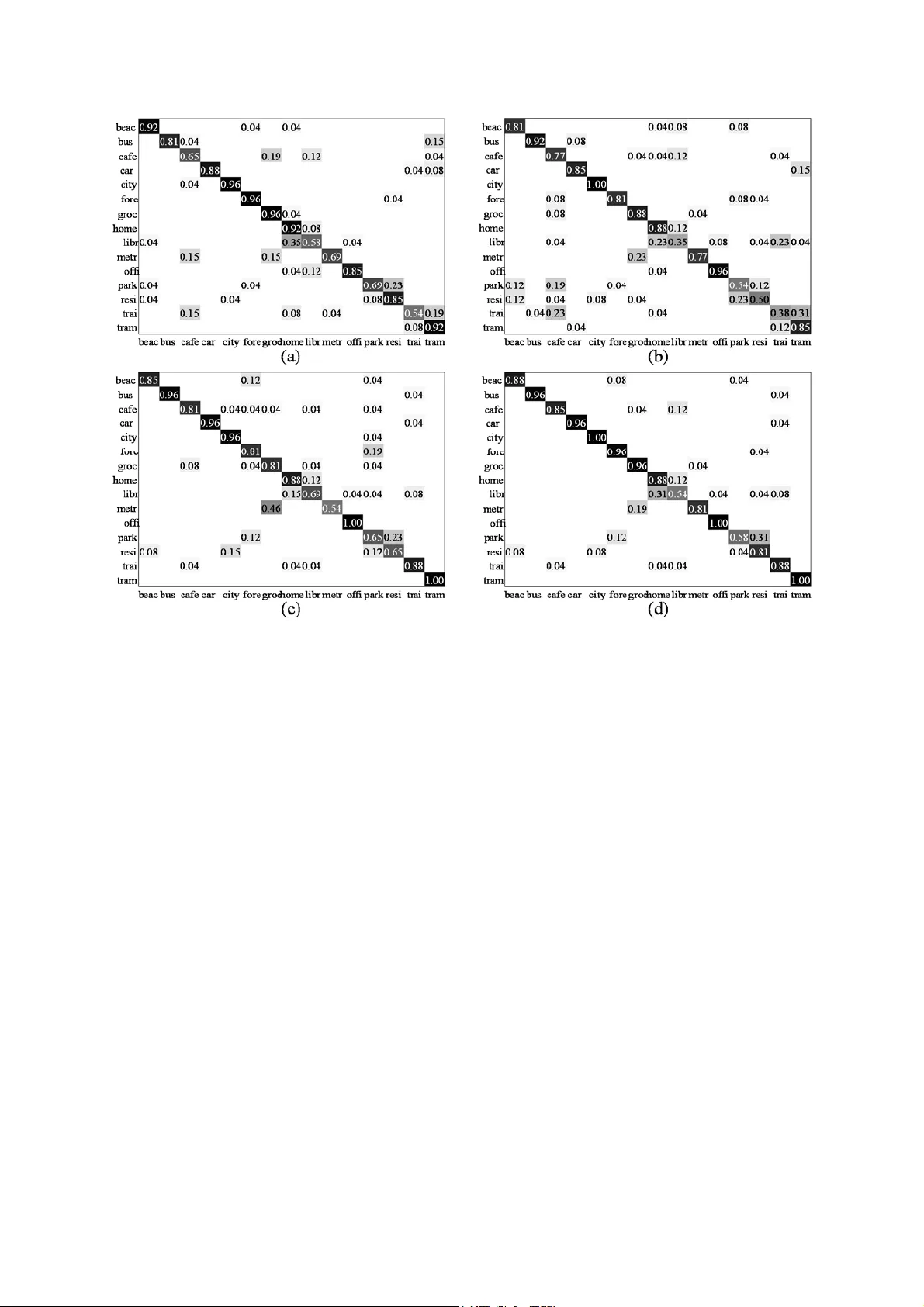
Analysis Acoustic Featur es for A coustic Scene Classification an d Scor e fusion of multi-classifica tion systems applied to DCASE 2 016 challenge Sangwook Park 1 , Seongkyu Mun 2 , Younglo Lee 1 , David K. Han 3 , and Hanseok Ko 1 1 School of Electrical Engineeri ng, Korea University, Seoul, Sout h Korea 2 Department of Visual Information Processing, Korea University, Seoul, South Korea 3 Office of Naval Resea rch, Arlington, VA, USA {swpark, skmoon, yllee}@ispl.korea.ac.kr, ctmkhan@gmail.com, hsko@korea.ac.kr Abstract This paper describes an acousti c scene classification method which achieved the 4 th r a n k i n g r e s u l t i n t h e I E E E A A S P challenge of Detecti on and Classification of Acoustic Scenes and Events 2016. In order to accomplish the ensuing task, several methods are e xplored in t hree aspects: feature extracti on, feature transformation, and score fusion for final decision. In the part of feature extraction, several features are investigat ed for effective acoustic sc ene cla ssification. For resolving the issue that the same sound can be heard in different places, a feature transformation is applied for better separation for classification. From these, several systems based on different feature sets are devised for classification. The final result i s determined by fusing the individual systems. The method is demonstrated and validated by th e experiment conducted using the Challenge database . Index Term s : acoustic scene classification, cepstral features, covariance learning, scor e fusion 1. Introduction Audio signal including speech, general sound (non-linguistic sound), and background sound m ay be quite informative in characterizing context such as presence o f humans, objects, their activities, or the enviro nment. Among these, location information is not only vital in multimedia analysis but also used in many tasks of obtaining c lues that are helpful in scene understanding. Location information is widely used i n many applications [1-2] including speech/acoustic event recognition as a pr ior fo r e nh an ci ng th e p erf ormance [3-4]. Thus, Acoustic Scene Classification (ASC) that recognizes the location where the observation is obtained has drawn considerable attention due to these usa ges. Typically, ASC system consists of feature extraction and classification. In fea ture extr action, observation data having discriminative chara cteristics depending on locations are expressed as a feature vecto r. Mel Frequency Cepstr al Coefficients (MFCCs) and Perceptual Linear Prediction (PLP) have been applied in early ASC s y s t e m . L o w - l e v e l s p e c t r a l features such as zero-crossing rate, spectral statistics, and timbre were employed for AS C by combining them with MFCCs [5]. Chu [6] utilized a joint feature between MFCCs and time-frequency features obt ained from the matching pursuit decomposition of acoustic sce nes to improve the overall performance. In other approaches, a feature vector is extracted by considering variations am ong the frames. A Bag-Of-Frames (BOF) method, which considers an acoustic scene as a set of bags of various sounds, was applied to ASC [7-9]. This approach used statistical dist ribution (e.g. histogram) as features, which represents the occurrence count of cepstral features, qu antized by a codebook like dictionary. In classification, location where the observation is obtained can be revealed by a discriminant func tion which is obt ained based on Gaussian Mixture Model (GMM) or Support Vector Machine (SVM) [1, 7]. Although many approaches were applied for ASC applications, these still suffer from problems in realistic environments. Even in a same place, a variety of acoustic sounds occur depending on presenc e of people, objects, and their behaviors. For an example, when a microphone is set in a café, different types of sound can be captured depending on happenings such as cleaning, cof fee grinding, or people talking . As such, feature vectors obtained in the café can be widely scattered in a feature space, although these vectors come from t h e s a m e p l a c e . O n t h e o t h e r h a n d , c o n v e r s a t i o n s c a n w e l l b e heard where ever there are people. As such, the feature vectors obtained from different locations may well be very close to eac h other. As illustrated by the example here, ASC for location classification is still very challen ging in realistic environme nts. The main contributions of this paper are to establish an improved framework and a method for ASC as follow: 1) analysis of signal components composing an acoustic scene signal, a nd investigation of several features in terms of their components, 2) investigation of a novel feature a nd feature transformation for resolving the issue of location classificati on from the same sound source in different locations, and 3) development of a fusion method based on each system output for improving the overa ll ASC performance. The remainder of this paper is organized as follows. Section 2 explains the a pproach with its motivation. Section 3 introduces ASC approach es. After a discussion on the experimental results, conclusions are drawn in the final sectio n. 2. Audio Signal Components All sounds including a backgrou nd noise and reverberation can b e a s i g n a l f o r A S C , b e c a u s e a l l o f t h e m a r e h e l p f u l f o r obtaining the location information. An input s ound can be categorized into three components: stationarity, quasi- stationary, and non-stationary according to time duration. As shown in figure 1, an engine sound of a bus can be obviously considered as a stationar y component. In case of break noise of a bus, however , t hese sounds are considered as a quasi-stationary component because it can be considered as a stationary for a moment. And many sounds that suddenly happens are frequently captured in a short period of time. Thus , they are considered as non-stationary. Figure 1: Sample spectrogram obtai ned in a “bus” that is released by the DCASE 2016. A stationary component is the primary factor for a target locational information. The others are secondary factors because most of these acoustic events depend on people/entities in the location, and their behavior. 3. Approaches for Acoustic Scene Classification The system propos ed here is depicted in figure 2 with three main parts; Feature Extraction (FE), Classification (CL), and Score Fusion (SF). The method s applied in the system are described in the following. Figure 2: System architectu re applied in DCASE 2016 3.1. Feature Extraction (FE) 3.1.1. PLP and MFCC MFCC and PLP have shown good performance in recognition. In ASC, both features are obtained under the condition that all of t he three stationarity-based components (stationary, quasi- stationary, non-stationary) are mixed. In the case of PLP, an equal loudness pre-emphasis is applied to approximate the result of frequency in tegration to the inequivalent sensitivity of human a uditory sense at differe nt frequencies [10]. Thus, discriminative characters in h igh frequency band are included in the process although the energy contribution in high frequency is rela tively low due to their rapid atten uation. 3.1.2. PNCC The procedure for the Power Norm alized Cepstral Coefficients (PNCCs) called Medium-time pow er bias subtraction is added in the signal enhancement method [11]. Since the stationary component is considered as a power-bias in the procedure, t he feature is extracted under the condition that the stationar y component is suppressed. 3.1.3. RCGCC The Robust Compressive Gamma -chirp filterbank Cepstral Coefficients (RC GCCs) was adde d as signal enhancement [12]. In o ur im plem ent atio n of RCGC C the fe atur es ar e ex trac ted by suppressing a stationary compone nt as in the case with the PNCC. Additionally the non-stationary components are enhanced by applying a smoothe d weight to the observation subband power. 3.1.4. SPCC Since many sounds are non-stat ionar y and highly dynamic, feature vectors extracted in a location may be widely scattered in the feature space. For resolving the issue, Subspace Projection Cepstral Coefficients (SPCC) is applied [13]. The rank of each subspace is determin ed by preserv ing 90% of data energy that is a summati on of all eigenvalues. Figure 3: Subband powers applied to each feature extraction method 3.1.5. Cepstral Comb ination For summary of previously menti oned features, figure 3 shows several subband powers that are i ntermediately obtained in each feature extraction using an observation depicted in figure 1. A subband power applied to MFCC is shown in fi gure 3(a) that is similar to the spectrogram representing the mixed components. Enhanced subband powers for PNCC and RCGCC is shown in figure 3(b) and figure 3(c), respectively. In these cases, a stationary component is diminish ed. In particular, the high frequency bands corresponding to non-stationary component are more noticeable in the enhanced subband power for RCGCC. Whether quasi-stationar y component will be reduced or not is determined by its time duration. Since sounds are c ontinuously changing according to situations such as human beh aviors and other sound sources, feature vectors extracted in every frame are widely spread in vector space, even though th e features are obtained from a common place. In order to com plement this issue, a nove l feature is als o applied. According to advantages of each method , a Cepstral Combination (CepsCom) that is made up of concatenating four feature s; MFCC, PNCC, RCGCC, and SPCC are used f or ASC. 3.2. Feature Transform ation and Clas sification To resolve the issue that the same sound source can be heard in many different places, feature transformation is considered. [t 6] Although the same sound in different locational settings can be closely mapped in a feature space, their feature distributions may be different e nough to distingui sh if they are observed in different places. R. Wang’ s method of Covariance Discriminative Learning (CDL) as a transformation is implemented here [14]. I n c l a s s i f i c a t i o n , G M M i s c o n s i d e r e d f o r f r a m e b a s e d features including PLP and the other cepstral features. Nearest Neighbor (NN) is used for the result of CDL. 3.3. Score Fusion Accuracies of each class may be different depending on the approach. Thus, overall averaging accuracy can be improved b y considering all outputs from se veral systems. AND, OR, and Majority Vote are some of the commonly used fusion rules. However, these approaches have equal confidences for all outputs from each individual s ystem, though one of the systems may show more reliable output for a certain class. The approach proposed here is by way of weighted fusion as the final result computed in (1) as 1 _a r g m a x N nn cc c n f inal result w s       (1) where c and n are ind exes about class and individual system. n c s and n c w is a score normalized into the interval [0, 1] and its reliability (i.e. weight) in each individual system. In GMM and NN, likelihood and distance margin are defined as t he score, respectively. N is the number of individual systems applied for score fusion. The weight n c w is defined as in     , | , n c g P Gc Oc wP G c O c P Gg O c       (2) where G and O are random variables meaning a ground truth and an output of an individual s ystem, respectively. The more outputs are confused with the class c , the lower the weight is applied to its score, even if the cl ass c is p erfectly recognized in an individual system. The weight can be determined from a confusion matrix obtained from th e training data used for each individual system. 4. Experiments 4.1. Database and Experimen t setting For performance assessment, the proposed system was performed with the database released for DCASE challenge 2016 [15]. The database consists of development and ev aluation dataset. Both include 15 acoustic scenes: namely bus , café / restaurant , car , city cente r , forest path , grocery store , home , lakeside beach , library , metro station , office , residential area , train , tram , and urban park. Firstly, performance assessm ent was conducted by using only the Development dat aset. In this case, training and test s ets were assigned with a ratio of 1:3, because the a mount of traini ng case is limited in comparison to the test cas e in a real situat ion. In the second experiment, Devel opment and Evaluation datasets were used for training and test, respectively. Note that th e weight used for score fusion i s determined in the training. For feature extraction, frames were d efined as 2048 samples with an overlap with the next frame for 1024 samples. Discrete Fourier transform was conducted with a 2048 points Hamming window. In case of PLP, 39 coe fficients including delta, acceleration, and energy were extracted by using HTK [16]. In the others; MFCC, PNCC, RCGCC, and SPCC, 60 co efficients including delt a and acceleration were extracted. In this case, CepsCom is a 240-dimensional vector. 4.2. Experiment results and Discussions 4.2.1. Development of ASC system The accurac ies according to cl asses are summarized in Table 1. Among the cepstral features, SPCC shows the best accuracy in most of the classes. In case of 5 classes, MFCC or PNCC is better than SPCC, and RCGCC shows the second best in city , grocery , train , and tram . An average accuracy of CepsCom shows better than the other cepstral features. Especially, clas s accuracy outperforms cepstral features that are elements of the CepsCom in beach , car , city , gro cery , offi ce , and tram , because the distance between confusable features is sufficiently extended to distinguish the features by expanding a featur e space. Note that the PLP is excluded from forming CepsCom Table 1. Accuracies of experiment using Deve lopment dataset; the number of mixture is set to 4 and 64 in PLP and others except CepsCom-CDL (denoted by “Ceps-CDL”) and Fusion, respectively. [%] Avg. beach bus cafe car city forest groc. home lib. metro office park resid. train tram MFCC 66.83 66.67 68.80 64.96 64.96 85.90 59.83 63.25 72.22 69.66 63.68 71.37 56.84 66.24 47.86 80.34 PNCC 63.59 69.23 50.85 77.35 68.80 79.49 52.14 66.67 54.27 71.37 62.82 60.26 57.26 64.10 46.58 72.65 RCGCC 63.65 62.82 55.98 64.10 64.53 84.62 55.56 75.21 50.43 70.94 63. 25 62.82 53.85 61.11 48.72 80.77 SPCC 71.51 58.97 82.05 60.68 82.05 83.76 61.97 76.92 82.48 72.22 81.62 70.51 50.85 76.07 51.28 81.20 CepsCom 73.99 70.09 74.79 72.65 85.04 88.89 61.97 86.32 76.92 71.37 76.07 74.79 55.13 75.64 50.00 90.17 Ceps-CDL 74.62 70.51 78.21 49.15 89.74 91.88 79.06 85.04 63.68 83.33 77.35 82.48 61.97 73.50 50.00 83.33 PLP 68.43 63.25 73.50 51.71 73.50 76.50 86.75 72.65 79.91 57.26 75.64 54.70 59.83 68.38 45.73 87.18 Fusion 76.36 68.80 75.64 61.54 91.88 85.04 85.90 79.49 79.91 79.91 90.60 76.07 49.57 78.21 57.69 85.04 because accuracy variation depending on the number of mixture is somewhat different to other cepstral f eatures [17] . When the CDL is applied, t he CepsCom shows the best result among all considered f eatures. Although the average accuracy of CepsCom-CDL is sim ilar to CepsCom-GMM, each class accuracy is different to each other as shown in Table 1. Also, PLP-GMM system shows a better accuracy in forest and home. Based on this fact, CepsCom-GMM, CepsCom-CDL, and PLP-GMM are used to make t he f i n a l d ec is io n . T h e r e s ul t of the fusion shows the best av erage accuracy among individual systems. In parti cular, accuracies of car, metro, residentia l, and train are better than individual systems applied to the fusion. Since a low weight for unreliable output from an individual system is applied to the fusion, the best candidate after the fusion may well be the second be st candidate in an individual sys tem. 4.2.2. Evaluation of ASC system From the previous experiment, three systems were evaluated with Evaluation dataset. In results, average accu racies of all individual systems are much better than the previous one, because the number of training data is increased a s much as fou r times. Confusion matrices of each individual system are summarized in figure 4. As show n in the figure, the P LP-GMM especially shows more than 95% accuracy in city , forest, and grocery, while three groups; home-library , park-residentia l , and train-tram are confused to each other. Although the CepsCom-GMM also suffers from confusions in these groups, the system shows better accuracies than PLP-GMM in bus , café , city , metro , and office . The CepsCom-CDL also shows better accuracies than PLP-GMM and CepsCom -GMM in several classes, and confusion problem train and tram is resolved. In the result of fusion method, the aver age accuracy is shown as 87.18%, which is an improvement of 5.90%, 12.05%, 6.10% compared to PLP-G MM, CepsCom-GMM, and CepsCom-CDL, respectively. As shown in figure 4(d), two groups; home-library and park-residential are still confused, but train-tram confusion is resolved by t he Ce ps Co m -C DL . I n several classes, accuracy is improved after applying the fusion method. In particular, a ccuracies of several clas ses are b etter or equal compared to the best accuracy among individual systems in café , car , metro , and train . 5. Conclusions This paper described the A SC method that ranked the 4 th in the first task of the IEEE AASP Challenge: DCASE 2016. Features such as PLP, MFCC, PNCC, RCGCC, a nd SPCC are investigated, and these features are applied for scene classification by means of GMM for performance evaluation. Also, CDL is applied for feature transformation. From the fact that each class has different accuracy according to classificat ion approaches, score fusion method is developed for making the final decision. In th e experiment , the challenge database is us ed for performance assessment, and th e results are summarized and discussed to demonstrate these approaches appli ed to DCASE challenge. Figure 4: Confusion matrices; (a) PLP-GMM (b) CepsCom-GMM (c) C epsCom-CDL (d) Fusion 6. References [1] W. Choi, S. Kim , M. Keu m, D. K. Han, and H. Ko, “Acoustic a nd visual signal based context awareness system for mobile application,” IEEE Trans. Consum. Electron. , vol. 57, no. 2, pp. 738-746, 2011. [2] K. Yamano and K. I tou, “Browsi ng audio life- log data using acoustic and location information,” in IEEE Int. Conf. Mobile Ubiquitous Computing, Systems, Services and Technologies , pp. 96-101, 2009. [3] T. Nishiura, S. Nakamura, K. Miki, and K. Shikano, "Environmental sound source identification based on hidden markov model for robust speech recognition," EURO SPEECH 2003, pp. 2157- 2160, 2003. [4] T. Heittola, A . Mesaros, A. Eronen, and T . Virtanen, "Context- dependent sound event detection," EURASIP Journa l Audio, Speech, and Music Processing , pp. 1-13, 2013. [5] A. J. Er onen, V. T. Peltonen, J. T. Tuom i, A. P. Klapuri, S. Fagerlund, T. Sorsa, G. Lorho, a nd J. Huopaniemi, "Audio-based context recognition," IEEE Trans. Audio, Speech, and Language Processing , vol. 14, no. 1, pp. 321- 329, 2006. [6] S. Chu, S. Narayanan, and C. J. Kuo, "E nvironmental sound recognition with time-fre quency audio features," IEEE Trans. Audio, Speech, and Language Processing , vol. 17, no. 6, pp. 1142- 1158, 2009. [7] V. Carletti, P. Foggia, G. Percannella, A. Saggese, N. Strisciu glio, and M. Vento, "Audio surveillan ce using a bag of aural words classifier," in IEEE I nt. Conf. on Advanced Video and Signal Based Surveillance , pp. 81-86, 2013. [8] J.-J. Aucouturier, B. Defreville , and F. Pachet, "The bag-of- frames approach t o audio pattern recognition: A sufficient mode l for urban soundscapes but not for polyphonic music," The Journal of the Acoustical Society of America , vol. 122, no. 2, pp. 881- 891, 2007. [9] S. Pancoast and M. Akbacak, "Bag -of-Audio-Words approach for multimedia event classif ication," in INTERSPEECH 2 012 , pp. 2105-2108, 20 12. [10] H. Hynek, “Perceptual linear pre dictive (PLP) analysis of speec h,” The Journal of the Acoustical Society of America, vol . 87, no. 4, pp. 1738-1752, 1990. [11] C. Kim and R. M. Stern, “Featur e e xtraction for robust speech recognition using a power-law nonlinearity and power-bias subtraction,” in INTER SPEECH 2009 , pp. 28-31, 2009. [12] M. J. Alam, P. Kenny, and D. O’Shaughnessy. “Robust feature extraction based on an asymmet ric level-dependent auditory filterbank and a subband spectrum enhancement tec hnique,” Digital Signal Processing , vol 29, pp. 147-157, 2014. [13] S. Park, Y . Lee, D. K. Han, a nd H. Ko, “ Subspace projection cepstral coefficients for noise robust acoustic event recogniti on ,” in IEEE International Conference on Acoustics, Speech and Signal Processing , pp. 761-765, 2017. [14] R. Wang, H. Guo, L. S. Davis, and Q. Dai, "Covariance Discriminative Learning: A Natural and Efficient Approach to Image Set Classification," in IEEE Computer Vision and Pattern Recognition 2012, pp. 2496-2503, 2012. [15] A. Mesaros, T. Heittola, and T. Virtanen, “TUT database for acoustic scene classificatio n and sound event d etection,” in European Signal Processing Conference 2016, pp. 1128-1132, 2016. [16] The HTK boo k Version 3.4 , Cambridge University Engineering Department, 2009. [17] S. Park, S. Mun,, Y. Lee, and H. Ko, “Score fusion of classification systems for acoustic scene classification,” Technical report in Detection and Classification of Acoustic Scenes and Events 2016.