Self-Estimation of Path-Loss Exponent in Wireless Networks and Applications
The path-loss exponent (PLE) is one of the most crucial parameters in wireless communications to characterize the propagation of fading channels. It is currently adopted for many different kinds of wireless network problems such as power consumption …
Authors: Yongchang Hu, Geert Leus
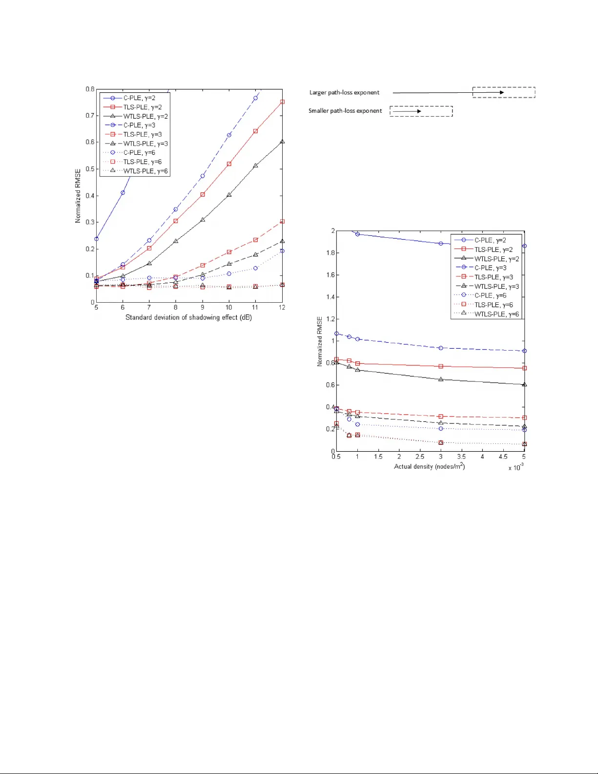
IEEE TRANSA CTIONS ON VEHICULAR TECHNOLOGY, VOL. 64, NO. 11, NO VEMBER 2015 5091 Self-Estimation of P ath-Loss Exponent in W ireless Networks and Applications Yo n g c h a n g H u , Member , IEEE , and Geert Leus , Fe l l o w, I E E E Abstract —The path-loss exponent (PLE) is one of the most crucial parameters in wireless communications to characterize the propagation of fading channels. It is currently adopted for many different kinds of wireless network problems such as power con- sumption issues, modeling the communication envir onment, and receiv ed signal strength (RSS)-based localization. PLE estimation is thus of great use to assist in wireless networking. However , am a j o r i t yo fm e t h o d st oe s t i m a t et h eP L Er e q u i r ee i t h e rs o m e particular information of the wireless network, which might be unknown, or some external auxiliary de vices, such as anchor nodes or the Global Positioning System. Moreover , this external inf orma- tion might sometimes be unreliable, spoofed, or difficult to obtain. Theref ore, a self-estimator for the PLE, which is able to work in- dependently , becomes an urgent demand to robustly and securely get a grip on the PLE for various wireless network applications. This paper is the first to introduce two methods that can solely and locally estimate the PLE. T o start, a new linear regression model for the PLE is presented. Based on this model, a closed-form total least squares (TLS) method to estimate the PLE is first proposed, in which, with no other assistance or external information, each node can estimate the PLE merely by collecting RSSs. Second, to suppress the estimation errors, a closed-form weighted TLS method is further developed, having a better performance. Due to their simplicity and independence of any auxiliary system, our two proposed methods can be easily incorporated into any kind of wireless communication stack. Simulation results show that our estimators are reliable, even in harsh en vironments, where the PLE is high. Many potential applications are also explicitly illustrated in this paper , such as secure RSS-based localization, k th nearest neighbor routing, etc. Those applications detail the significance of self-estimation of the PLE. Index T erms —Lognormal shadowing, path-loss exponent (PLE), radio propagation channel, security, total least squares (TLS). I. I NTR ODUCTION I N WIRELESS communications, the receive d instantaneous signal power at receiv ers is commonly modeled as the prod- uct of large-scale path-loss and small-scale fading. Large-scale path-loss fading assumes that the attenuation of the av erage receiv ed po wer is subject to the transmitter–receiv er distance r as r γ ,w h e r e γ is the path-loss exponent (PLE). Due to the Manuscript receiv ed March 21, 2014; revised August 8, 2014; accepted December 5, 2014. Date of publication December 10, 2014; date of current vers ion Novem ber 10, 2 015. Th is work wa s sup po rt ed by t he C hin a Sc ho lar sh ip Council (CSC) and Circuits and Systems (CAS) Group, Delft Univ ersity of T echnology , Delft, The Netherlands. The revie w of this paper was coordinated by Prof. T . Kuerner The authors are with the Faculty of Electrical Engineering, Mathematics, and Computer Science, Delft Univ ersity of T echnology, 2628 CD Delft, The Netherlands (e-mail: Y .Hu-1@tudelft.nl; G.J.T .Leus@tudelft.nl). Color versions of one or more of the figures in this paper are available online at http://ieeexplore.ieee.org. Digital Object Identifier 10.1109/TVT .2014.2380823 dynamics of the communication channel, the PLE varies ov er different scenarios and different locations. At the same time, small-scale fading constitutes a rapid fluctuation around the aver a g e o f t he r e ce ive d pow e r a n d fo l l ows a st o c ha s t ic p ro c e ss . It is mainly due to the multipath effect and changes over very small distances and very small time intervals. Howe ver , it can generally be well suppressed by means of some special receiv er designs and digital signal processing. Therefore, the PLE becomes a key parameter in characterizing the propagation channel, which significantly determines power consumption, quality of a transmission link, efficienc y of packet delivery , etc. It is important to accurately estimate the PLE so that the wireless communication stack can be dynamically adapted to the PLE changes to yield a better performance. For instance, a path with a relatively lo w PLE can be chosen to route messages to sa ve power . The PLE is also significant for some other applications. For instance, to calculate the location of a target node in recei ved signal strength (RSS)-based localization, ac- curate PLE estimation is required, which is mostly provided by reference nodes with known positions. Howe ver , in some cases, the reference nodes might be broken and cannot talk to the target node or the location information of the reference nodes might be unreliable, or spoofed by an adversary . Then, accurately estimating the PLE will become a difficult task. Current methods to estimate the PLE either require some information of the wireless network, which is unknown in most cases, or assistance from auxiliary systems. Three algorithms are presented in [1]: First, when network density is known, the PLE can be estimated by observing RSSs during sev eral time slots and by calculating the mean interference; with regard to the other two algorithms, by changing the r eceiv er’ s sensitivity , the PLE can be estimated either from the corresponding virtual outage probabilities or from the corresponding neighborhood sizes. All three algorithms require knowledge of the network density or the receiv er settings, and even require changing them. Other methods to estimate the PLE mostly lie in the area of RSS-based localization. As already mentioned, using the RSSs for localization requires an accurate estimate of the PLE, which is tightly related with the transmitter–receiv er distance. Therefore, special reference nodes with known po- sitions, namely , anchor nodes, are strategically predeployed with the purpose of calibrating the PLE [2]. Considering that the transmitter–receiver distances between anchor nodes can be difficult or expensiv e to accurately measure in some envi- ronments, the PLE can also be estimated by using receiv ed power measurements and geometric constraints of anchor nodes to avoid the distance calculation [3]. In the meantime, much 0018-9545 © 2014 IEEE. T ranslations and content mining are permitted for academic research only . Personal use is also permitted, but republication/ redistribution requires IEEE permission. See http://www .ieee.org/publications_standards/publications/rights/index.html for more information. 5092 IEEE TRANSACTIONS ON VEHICULAR TECHNOLOGY, VOL. 64, NO. 11, NO VEMBER 2015 effort has been put to jointly estimate the location and the PLE [4]–[6]. Some other methods start with an initial guess of the PLE to approximate the location, which is then used to update the PLE estimate [ 7], [8]. Howe ver , all those methods basically rely on the information from anchor nodes or other auxiliary systems. Once such systems are attacked, una v ailable, or generate large errors, the impact on the whole system will be unimaginable. Furthermore, the giv en methods are also not feasible for many kinds of wireless networks, in which commu- nications and information exchanges might be highly restricted. Therefore, a new self-estimator of the PLE is urgently required, which can solely and locally estimate the PLE without relying on any external assistance. Such an estimator should be able to not only serve localization techniques but act as a general method that can be easily incorporated into any kind of wireless network and any layer of the communication stack as well. The rest of this paper is structured as follows. In Section II, we present the s ystem model considered in this paper and discuss the problem statement. Some new parameters are intro- duced in Section I II to build a linear regression model for the PLE. Section IV presents and discusses the derivation of our two proposed PLE estimators. Simulation results are given and analyzed in Section V. Many potential applications are dis- cussed in Section VI. Section VII finally summarizes this paper . II. S YSTEM M ODEL Here, we introduce some important system model concepts and additionally describe the problem statement. A. Node Distribution Due to the unkno wn topology of wireless networks, partic- ularly in wireless ad hoc networks, neighbors of a node are ideally considered randomly deployed within the transmission range, indicated by W .I no t h e rw o r d s ,al o c a lr a n d o mr e g i o n around the considered node is assumed. Therefore, the proba- bility of finding k nodes in a subset Ω ⊂ W is giv en by P [ k nodes in Ω ] = n ! k !( n − k )! ! µ ( Ω ) µ ( W ) " k ! 1 − µ ( Ω ) µ ( W ) " n − k (1) where P denotes probability , n is the neighborhood size in W , and µ ( · ) is the standard Lebesgue measure. If we let Ω be a d -dimensional ball of radius r originating at the considered node, µ ( Ω ) is the volume of Ω and is giv en by µ ( Ω ) = c d r d , where c d = π d 2 Γ ( 1 + d/ 2 ) (2) with Γ ( · ) the gamma function. When d = 1 , 2o r3 , c d = 2 , π and ( 4 / 3 ) π ,r e s p e c t i v e l y .F o re x a m p l e ,w i r e l e s sv e h i c u l a rn e t - work s c an be mo del ed in 1-D s pac e, a fl at- Ea rth mo de l r equ ire s d = 2, and wireless unmanned aerial vehicle communications requires d = 3. In this paper , all formulas are generalized in a d -dimensional manner for the sake of theoretical consistency . Fig. 1. Impact of the shadowing effect on node A . ˆ n is the estimate of the theoretical neighborhood size n by counting the reachable neighbors, i.e., ˆ n = n + ∆ n . By ranking the recei ved powers at A ,t h ec o r r e s p o n d i n gr a n k i n g numbers ˆ i are the estimate of the ranking numbers i of the ranges, where ˆ i = i + ∆ i . B. Channel Model The attenuation of the channel can be modeled as comprised of large-scale fading, the shado wing ef fect, and small-scale fadi ng. La rge-s cal e fadi ng ind ica tes t hat th e emp iri cal de ter- ministic reduction in power density of an electromagnetic wave is exponentially associated with the distance when it propagates through space. W e assume that the transmitted power P t is reduced through the propagation channel ov er a distance r ,s u c h that the RSS P r is giv en by P r = C 1 P t # r 0 r $ γ (3) where r 0 ≪ r is the reference distance related to far-field, and C 1 is a nondistance-related constant that depends on the carrier frequency , the antenna gain, and the speed of light. P r and P t are both expressed in watts . Depending on the en vironment, the PLE γ ranges from 2 to 6 [9]. Obstacles, such as trees, buildings, and so forth, cause the actual attenuation of the received po wer to follow a lognormal distribution, which is also called the shadowing ef fect. As such, (3) has to be changed into ∆ P = 10 γ log 10 ( r ) − 10 log 10 ( C 1 ) − 10 γ log 10 ( r 0 )+ χ (4) where ∆ P = 10 log 10 ( P t /P r ) in decibels indicates the at- tenuation of the signal strength, and χ follows a zero-mean Gaussian distribution with standard deviation 2 < σ < 12. T o serve the following deri vations, two sev ere consequences of the shadowing effect should be mentioned. 1) The theoretical neighborhood size n is different from the actual neighborhood size ˆ n = n + ∆ n .A ss h o w ni n Fig. 1 for d = 2, the dashed regular circle is the theoret- ical transmission range of node A .I nf a c t ,p a c k e t s c a n be successfully receiv ed under the condition that P r > P thres ,w h e r e P thres is the receiver’ s sensitivity . Due HU AND LEUS: SELF-ESTIMA TION OF P A TH-LOSS EXPONENT IN WIRELESS NETWORKS AND APPLICA TIONS 5093 to the shadowing ef fect, the actual transmission range is irregular , as indicated by the solid line. 2) Another consequence caused by the shadowing effect is that after ranking all the receiv ed powers at node A , the node with the ˆ i th strongest the receiv ed power P r, ˆ i corresponds to the i th nearest neighbor at distance r i , where ˆ i = i + ∆ i . When signals are being transmitted, scatterers and reflectors create several reflected paths that reach the receiver , in addition to the line of sight. This is called small-scale fading, which is nondistance related. The instantaneous recei ved signal env elope follows the Nakagami- m distribution [10], and the distribution of the instantaneous received power p is, hence, given by P ( p )= # m E ( p ) $ m p m − 1 e − mp E ( p ) Γ ( m ) (5) where m is the fading parameter, and a small value of m indicates more fading. The measured received power P r can be obtained by taking the av erage ov er K consecutiv e time slots of the instantaneous received power p k ,i . e . , P r = ( 1 /K ) % K k =1 p k ,a n dt h u s , Va r ( P r )=[ E ( p k )] 2 /K m . When K is large enough, the impact of small-scale fading can be greatly eliminated. Additionally , a well-designed receiv er is able to suppress the multipath effect to a great degree by using special antenna designs such as a choke ring antenna, a right- hand circularly polarized antenna, etc. Therefore, the power attenuation model in this paper is mostly subject to large-scale fadi ng and sh adowi ng, an d hen ce, we w ill re ly on (4 ) i n t he re st of this paper . C. Pr oblem Statement We a r e n o w a i m i n g a t d e v e l o p i n g a n e w s e l f - e s t i m a t o r o f t h e PLE. The desired properties of the proposed estimator can be summarized as simple , pervasive , local , sole , collective ,a n d secur e . Simple indicates that the proposed estimator should be easy to implement and carry out. P ervasive signals that it can be incorporated into any kind of network regardless of its design. Therefore, the only freedom left for us is to utilize the RSS. Some kind of networks might not have any external auxiliary system or access to external information, and their mutual nodal cooperations might be severely constrained. Moreov er , even if there are no such constraints, adversaries can easily tamper with or forge the exchanged critical information. This requires that the estimator has to run solely on a single node by collecting the locally receiv ed signal strengths. By this means, a PLE can be secur ely and locally estimated. As is shown in (3), the PLE γ is strictly subject to the power attenuation and the transmitter–receiv er distance. Therefore, con ventional estimators in wireless localization try to obtain the PLE by introducing anchor nodes to fix the transmitter–receiv er distance and by observing power attenuations. Howe ver , the desired properties of the proposed estimator determine that it is not possible to fix or to know exact transmitter–receiv er distances of some of the collected RSSs. As such, we can define the problem as “How can we estimate the PLE γ without knowing transmitter–receiv er distances, i.e., merely from the local RSSs?” III. L INEAR R EGRESSION M ODEL FOR THE P AT H -L OSS E XPONENT To s o l v e t h e p r e v i o u s l y m e n t i o n e d p r o b l e m , w e i n t r o d u c e some ne w parameters. After estimating those parameters, a new linear regression model for the PLE is presented. A. Ranking RSSs Let us focus on a single node and denote P r, ˆ i as the ˆ i th strongest power receiv ed at the considered node, where ˆ i = 1 , 2 ,..., ˆ n ,i . e . , P r, 1 ≥ P r, 2 ≥ · · · ≥ P r, ˆ n and r i as the i th clos- est range to the considered node, where i = 1 , 2 ,...,n ,i . e . , r 1 ≤ r 2 ≤ · · · ≤ r n .A sw em e n t i o n e de a r l i e r , ˆ i = i + ∆ i is considered as an estimate of i ,w h e r e ∆ i is called the mismatch. From (4), we can then write ∆ P ˆ i = 10 γ log 10 ( r i ) − C 2 + χ i (6) where χ i ∼ N ( 0 , σ 2 ) , ∆ P ˆ i = 10 log 10 ( P t /P r, ˆ i ) ,a n d C 2 = 10 log 10 ( C 1 )+ 10 γ log 10 ( r 0 ) is a constant. W e assume that all neighboring nodes transmit signals with the same power P t such that the ordered values of P r, ˆ i lead to the ordered values of ∆ P ˆ i ,i . e . ,w ec a na s s u m et h a t ∆ P 1 ≤ ∆ P 2 ≤ · · · ≤ ∆ P ˆ n . Admittedly , in a more realistic situation, the transmit power P t at each neighboring node might be different. Howe ver , our proposed estimators can still remain feasible in such a case, and we will come back to this issue in Section IV -D. B. Linear Re gr ession Model for the PLE From (6), we notice that ∆ P ˆ i is a function of P t and C 2 , which are both unknown. Howe ver , these can be canceled by subtracting ∆ P ˆ j from ∆ P ˆ i ,l e a d i n gt o ∆ P ˆ i, ˆ j = ∆ P ˆ i − ∆ P ˆ j = 10 log 10 ( P r, ˆ j /P r, ˆ i ) ,w h i c hc a nf u r t h e rb ew r i t t e na s ∆ P ˆ i, ˆ j = 10 γ log 10 ( r i ) − 10 γ log 10 ( r j )+ χ i,j = 10 γ log 10 ! r i r j " + χ i,j (7) where χ i,j ∼ N ( 0 , 2 σ 2 ) . Now , we define L i = 10 log 10 ( r i ) as a logarithmic function of r i ,a n dh e n c e , L i,j = L i − L j = 10 log 10 ( r i /r j ) .T h u s ,( 7 ) becomes ∆ P ˆ i, ˆ j = γ L i,j + χ i,j . (8) It is already apparent that if L i,j can be estimated, a linear re- gression model for the PLE can be constructed from (8). Let us denote & L ˆ i, ˆ j as the estimate of L i,j and ε ˆ i, ˆ j as the corresponding estimation error . The linear regression model is then giv en by ∆ P ˆ i, ˆ j = γ ( & L ˆ i, ˆ j − ε ˆ i, ˆ j )+ χ i,j . (9) C. Estimation of L i,j As discussed in the problem statement, it is not possible to directly obtain the transmitter–receiver distances if the estimat- ing node solely and locally collects the RSSs. Therefore, the idea of ranking the RSSs is crucial for our method. 5094 IEEE TRANSACTIONS ON VEHICULAR TECHNOLOGY, VOL. 64, NO. 11, NO VEMBER 2015 Fig. 2. In 2-D space when the shadowing ef fect does not impact the ranking, i.e., ˆ i = i ,t h es o l i dc i r c l es h o w st h et r a n s m i tr a n g eo fr a n d o mn o d e A ,w h e r e A receives 12 signal strengths from its neighbors. Its third and sixth closest neighbors lie on the dotted circles, which have r 3 and r 6 as radii, respectively . Therefore, r 3 has three nodes inside, whereas r 6 has six nodes inside. P r, 3 and P r, 6 are, respectiv ely , the third and sixth strongest receiv ed power . ∆ P 3 , 6 = 10 log 10 ( P r, 6 /P r, 3 ) ,a n d & L 3 , 6 =( 10 / 2 )l o g 10 ( 3 / 6 ) ≈− 1.505. Likewise, other pairs of ∆ P ˆ i, ˆ j and & L ˆ i, ˆ j can be obtained. By ranking the values of P r, ˆ i ,w eo b t a i nt h er a n k i n g n u m b e r ˆ i ,w h i c hw i l lb ef u r t h e ru s e dt oe s t i m a t et h er a n k i n gn u m b e r s i of the ranges, where we recall that ˆ i = i + ∆ i .A d d i t i o n a l l y ,i t is obvious that i indicates the number of nodes within the ball of radius r i ,w h i c hc a nb ef u r t h e re x e m p l i fi e di nF i g .2 .T h e r e f o r e , the essence of the proposed method is to use the rank numbers of ˆ i as new measurements to estimate the values of L i,j . Note that L i,j is a linear combination of L i and L j .W e focus on estimating L i ,a n dt h ee s t i m a t eo f L j can be obtained like wise. Considering (1) and (2), the probability mass function of finding i nodes within the d -ball of radius r i ,w h i c hi sp a r a m e - terized by L i = 10 log 10 ( r i ) ,c a nb ew r i t t e na s P [ i | L i ]= n ! i !( n − i )! ' c d 10 dL i 10 µ ( W ) ( i ' 1 − c d 10 dL i 10 µ ( W ) ( n − i . (10) Based on (10), to find the maximum likelihood (ML) estimator & L i ,w en e e d t of o r c et h ed e r i v a t i v eo fo u rl i k e l i h o o df u n c t i o nt o zero by ∂ ln ( P [ i | L i ]) ∂ L i = 0 . (11) Therefore, by solving (11), the ML estimator & L i can be easily obtained as & L i = 10 d log 10 ! iµ ( W ) nc d " . (12) Like wise, & L j can be obtained, and the estimate of L i,j is, hence, giv en by & L i,j = 10 d log 10 ! i j " = L i,j + ε i,j (13) where ε i,j is the estimation error of & L i,j .P l u g g i n g ˆ i = i + ∆ i and ˆ j = j + ∆ j into (13), we have & L ˆ i, ˆ j = 10 d log 10 ' ˆ i ˆ j ( = L i,j + ε ˆ i, ˆ j (14) ε ˆ i, ˆ j = ε i,j + ∆ ε i,j (15) where ∆ ε i,j = & L ˆ i , ˆ j − & L i,j =( 10 /d )l o g 10 ((( i + ∆ i ) /i )( j/ ( j + ∆ j ))) . From (13) and (14), we ev en notice that µ ( W ) , n ,a n d c d disappear after subtraction. This makes the proposed estimators only subject to the RSSs and the rank numbers in d -dimensional space. IV . P AT H -L OSS E XPONENT E STIMA TION To s o l v e t h e l i n e a r r e g r e s s i o n m o d e l , t h e t o t a l l e a s t s q u a r e s (TLS) method helps us obtain the estimate of the PLE γ . Howe ver , the general solution to the TLS method turns out to be time consuming. Therefore, a closed-form solution is provided, saving computational time tremendously . Moreover , a closed- form weighted TLS method is further proposed to suppress the estimation errors, yielding a better performance. A. TLS Solution As for the example in Fig. 2, node A computes ∆ P ˆ i, ˆ j and estimates & L ˆ i, ˆ j for all pairs of nodes within its range, i.e., ˆ i, ˆ j = 1 , 2 , 3 ,..., ˆ n .H o w e v e r ,f r o m( 9 ) ,w en o t i c et h a tt h eR S S sa r e corrupted by shadowing, and the values of & L ˆ i, ˆ j are measured with errors. Therefore, the TLS method is utilized to obtain our estimate, i.e., & γ tls [11]. We a s s u m e t h a t t h e c o n s i d e r e d n o d e h a s ˆ n neighbors, and all RSSs from its neighbors are ranked. Thus, we have a sample set of ∆ P ˆ i, ˆ j val u e s w h o s e s i z e i s N = ) ˆ n 2 * in total. W e vectorize the collected samples of ∆ P ˆ i, ˆ j and the corresponding values of & L ˆ i , ˆ j ,w h i c ha r e ,r e s p e c t i v e l y ,r e p r e s e n t e db yt h e N × 1v e c t o r s ∆ P and & L .T h e n ,( 9 )c a nb er e w r i t t e na s ∆ P = γ ( & L − E )+ X (16) where E and X are, respectiv ely , the N × 1v e c t o r so b t a i n e d by stacking the estimation errors ε ˆ i, ˆ j on & L ˆ i, ˆ j and the shado wing parameters χ i,j .T h eb a s i ci d e ao ft h eT L Sm e t h o di st ofi n da n optimally corrected system of equations ∆ P tls = γ & L tls with ∆ P tls := ∆ P − X tls , & L tls := & L − E tls ,w h e r e X tls and E tls are, respectively , optimal perturbation vectors. Therefore, the PLE estimate & γ tls for γ is the solution to the optimization problem { & γ tls , X tls , E tls } := arg min γ , X , E ∥ [ XE ] ∥ 2 F (17) subject to (16), where ∥ · ∥ F is the Frobenius norm. By changing (16) into + ( & L − E )( ∆ P − X ) , - γ − 1 . = 0( 1 8 ) we see that this is a typical low-rank approximation problem where the rank of the augmented matrix [ & L ∆ P ] should be optimally reduced to 1. HU AND LEUS: SELF-ESTIMA TION OF P A TH-LOSS EXPONENT IN WIRELESS NETWORKS AND APPLICA TIONS 5095 Therefore, we compute the singular v alue decomposition (SVD) of [ & L ∆ P ] , resulting in [ & L ∆ P ]= U Σ V T where V can be explicitly expressed as V = - V 11 V 12 V 21 V 22 . . Based on the Eckart–Y oung theorem [12], the estimated PLE is then giv en by & γ tls = − 1 V 22 V 21 . (19) B. Closed-F orm TLS Estimation The SVD-based method discussed in the previous section provides a general solution to the TLS problem. Ho we ver , considering the complexity brought by the SVD when process- ing a tremendous number of samples, a simplified method is required. Noting the linearity of (16) and the fact that the TLS method minimizes the orthogonal residuals, we can reformulate the TLS cost function as J tls = ∥ ∆ P − γ & L ∥ 2 1 + γ 2 . (20) By solving ∂ J tls ∂γ = γ 2 & L T ∆ P + γ ( & L T & L − ∆ P T ∆ P ) − & L T ∆ P ( 1 + γ 2 ) 2 = 0 (21) we obtain two solutions, which are, respecti vely , given by & γ 1 = η + / 1 + η 2 > 0( 2 2 ) & γ 2 = η − / 1 + η 2 < 0( 2 3 ) where η =( ∆ P T ∆ P − & L T & L ) / 2 & L T ∆ P . In fact, optimizing (20) can also be vie wed as finding a linear curve with slope γ through the origin, in which the values of P ˆ i, ˆ j and the values of & L ˆ i, ˆ j are, respectiv ely , on the y -axis and the x -axis. See [13] for some other TLS solutions to different modified linear regression models. Therefore, it is evident that two perpendicular curves are obtained, i.e., & γ 1 & γ 2 = − 1. One of the solutions minimizes J tls ,w h e r e a st h eo t h e rm a x i m i z e si t . Considering that & γ tls > 0, the TLS-PLE estimate is obviously giv en by & γ tls = & γ 1 . As far as computational complexity is concerned, the SVD procedure on [ & L ∆ P ] requires a complexity of approximately 8 N 2 to obtain U , Σ ,a n d V [14]. If only V is required to estimate the PLE, the SVD-based method still has a complexity of approximately 16 N .H o w e v e r ,o u rc l o s e d - f o r ms o l u t i o nh a s only a complexity of approximately 3 N . Compared with the SVD-based solution, we also measure the average computational time when the transmission range is 200 m. The methods are implemented in MA TLAB 2012b on a Lenov o IdeaPad Y570 Laptop (Processor 2.0 GHz Intel Core i7, Memory 8 GB). As s hown in Fig. 3, the computational time of Fig. 3. Computational time of the traditional solution and the closed-form solution. the closed-form solution is greatly reduced particularly when the sample size is increased. C. Closed-F orm W eighted TLS Estimation From the aforementioned analyses, we can conclude that there are three kinds of errors impacting the PLE estimate. 1) The estimation error ε i,j on & L i,j is subject to the spatial dynamics of the node deployment. Therefore, when in- creasing the actual density , such errors will be decreased. 2) The shadowing effect introduces a Gaussian error χ i,j , which will decrease when the sample size is increased. 3) The last kind of error is ∆ ε i,j ,w h i c hr e p r e s e n t st h e mismatch between the r anking numbers of the receiv ed power and the ranges. This kind of error is subject not only to shado wing but also to the spatial dynamics of the nodes. When the actual density is increased and the nodes get closer to each other , the differences of the received power become relatively small, which leads to a large impact of shadowing on the ranking. We p r o p o s e a w e i g h t e d T L S m e t h o d t a r g e t i n g t h e s u p p r e s - sion of ∆ ε i,j .P l u g g i n g ˆ i = i + ∆ i and ˆ j = j + ∆ j into ∆ ε i,j , we hav e ∆ ε i,j = 10 d log 10 ' ˆ i ˆ i − ∆ i ( − 10 d log 10 ' ˆ j ˆ j − ∆ j ( . (24) By using some bounds of the natural logarithm, i.e., 1 − ˆ i − ∆ i ˆ i ≤ ln ' ˆ i ˆ i − ∆ i ( ≤ ˆ i ˆ i − ∆ i − 1( 2 5 ) where equality is obtained when ∆ i = 0, bounds for ∆ ε i,j can be computed as 10 ln( 10 ) d ' 2 − ˆ i − ∆ i ˆ i − ˆ j ˆ j − ∆ j ( ≤ ∆ ε i,j ≤ 10 ln( 10 ) d ' ˆ i ˆ i − ∆ i + ˆ j − ∆ j ˆ j − 2 ( . (26) 5096 IEEE TRANSACTIONS ON VEHICULAR TECHNOLOGY, VOL. 64, NO. 11, NO VEMBER 2015 Fig. 4. TLS weights as a function of ˆ i for ˆ n = 100 and ˆ j = 50. Considering that 1 ≤ ˆ i − ∆ i ≤ ˆ n and 1 ≤ ˆ j − ∆ j ≤ ˆ n ,w e can further bound ∆ ε i,j as 10 ln( 10 ) d ! 2 − ˆ i − ˆ n ˆ j " ≤ ∆ ε i,j ≤ 10 ln( 10 ) d ! ˆ n ˆ i + ˆ j − 2 " . (27) From (27), we can finally find an upper bound of ∆ ε 2 i,j as ∆ ε 2 i,j ≤ 100 ln( 10 ) 2 d 2 max 0 ! ˆ n ˆ i + ˆ j − 2 " 2 , ! ˆ n ˆ j + ˆ i − 2 " 2 1 . (28) The idea is now to assign a large weight to a sample with a small upper bound of the mismatch ∆ ε 2 i,j .T h e r e f o r e ,b a s e do n (28), the weights can be constructed by ω i,j = 1 max 2 # ˆ n ˆ i + ˆ j − 2 $ 2 , # ˆ n ˆ j + ˆ i − 2 $ 2 3 . (29) We p l o t t h e w e i g h t s w h e n ˆ j = 50 and ˆ n = 100 in Fig. 4. By stacking the values of ω i,j on the diagonal of a diagonal matrix in the same way we stack the values of ∆ P ˆ i, ˆ j and the val u e s o f & L ˆ i, ˆ j ,w ec o n s t r u c tt h e N × N weight matrix W ,a n d then, the weighted TLS cost function can be constructed by J wtl s = ( ∆ P − γ & L ) T W ( ∆ P − γ & L ) 1 + γ 2 . (30) As before, the closed-form weighted TLS-PLE (WTLS-PLE) estimate is then easily given by & γ wtl s = η ′ + / 1 + η ′ 2 (31) where η ′ =( ∆ P T W ∆ P − & L T W & L ) / 2 & L T W ∆ P . D. Discussions and Future W orks Here, we discuss some remaining theoretical problems and some possible issues related to real-life environments. Mean- while, we cast light on our future works. 1) CRLB: The Cramér–Rao lower bound (CRLB) is very difficult to obtain for this problem. This is due to the fact that the estimation accuracy of the PLE is subject to the spatial dynamics, the shadowing, and the rank number estimate. They are all mutually related, particularly for the ranking number estimate, which does not follow any known probability density function (pdf). That is also why we selected a bound on the error to construct the weights to suppress the mismatch of the ranking numbers. In our future work, we are looking for one-step estimation methods that can directly utilize the RSSs without the ranking procedure. T o achiev e that, a pdf of the RSS in an ad hoc en vironment is required, which considers spatial dynamics and shadowing. Based on such a pdf, a better estimator , such as the ML estimator , and the CRLB can be introduced. 2) Differ ent T ransmit P ower V alues: Previously , we assume the same transmit power P t for all the neighboring nodes, which might not be so realistic. Howe ver , assume now that the transmit power values are dif ferent. W e then have to particularly estimate the transmit power P t, ˆ i from the ˆ i th node to calculate the path loss ∆ P ˆ i := 10 log 10 ( P t, ˆ i /P r, ˆ i ) and further compute ∆ P ˆ i, ˆ j := ∆ P ˆ i − ∆ P ˆ j .O t h e r w i s e ,i fw es t i l lc o m p u t e ∆ P ˆ i, ˆ j := 10 log 10 ( P r, ˆ j /P r, ˆ i ) ,o u re s t i m a t o r sw i l lb e c o m ew o r s ey e ts t i l l feasible. T o see that, we first need to assume an unknown aver a g e t r an s m it powe r ¯ P t and, hence, use 10 log 10 ( P t, ˆ i )= 10 log 10 ( ¯ P t )+ ∆ P t, ˆ i ,w h e r e ∆ P t, ˆ i is the deviation in decibels of the transmit power from the ˆ i th node. Then, (9) has to be changed into ∆ P ˆ i, ˆ j = γ ( & L ˆ i, ˆ j − ε ˆ i, ˆ j )+ χ i,j + ∆ P t, ˆ i, ˆ j (32) where ¯ P t can still be canceled, and ∆ P t, ˆ i, ˆ j := ∆ P t, ˆ i − ∆ P t, ˆ j . Obviously , although X in (16) has to become the vector of χ i,j + ∆ P t, ˆ i, ˆ j val u e s , o u r p r o p o s e d e s t i m a t o r s c a n s t i l l e s t i m a t e the PLE since the general form of (16) remains the same. Hence, if we assume that ∆ P t, ˆ i, ˆ j is Gaussian distributed, χ i,j + ∆ P t, ˆ i, ˆ j is still a zero-mean Gaussian variable, which means that the different transmit power values can equiv alently be considered as a more se vere shadowing impact. Therefore, for conv enience, we still assume the same transmit power in this paper . 3) Dir ectional PLE Estimation: Another practical problem is that the PLE sometimes varies ov er different directions while we previously assume that the PLE is omnidirectionally the same. T o cope with this problem, we discuss and can extend our proposed estimators with a directional PLE estimation. As shown in Fig. 5, we assume that only the RSSs from the nodes within the angular window φ are subject to the same PLE. Hereby in (1), W has to become the actual transmission range bounded by the angle φ ,e . g . , W φ ,w h e r e a s Ω becomes the corresponding sector Ω φ with radius r .T h ev o l u m eo f Ω φ then becomes µ ( Ω φ ): = c d, φ r d ,w h e r ef o r d = 1 , 2 , 3, we have c 1 , φ := 1, c 2 , φ := φ / 2, and c 3 , φ := ( 2 π / 3 )( 1 − cos φ ) .S i n c e HU AND LEUS: SELF-ESTIMA TION OF P A TH-LOSS EXPONENT IN WIRELESS NETWORKS AND APPLICA TIONS 5097 Fig. 5. Demonstration of the directional PLE estimation in R 2 . A is the con- sidered node collecting the RSSs from within the angle φ . W φ is the actual transmission range bounded by φ ,a n dt h es h a d e da r e a Ω φ is the corresponding sector with radius r . the nodes are still randomly deployed within W φ ,c o m p a r e d with (10), we can, hence, similarly write P [ i | L i ]= n ! i !( n − i )! ' c d, φ 10 dL i 10 µ ( W φ ) ( i ' 1 − c d, φ 10 dL i 10 µ ( W φ ) ( n − i . (33) Although the estimate of L i has to be changed into & L i = 10 d log 10 ! iµ ( W φ ) nc d, φ " (34) the estimate of L i,j ,h o w e v e r ,r e m a i n st h es a m e ,i . e . , ˆ L i,j := ˆ L i − ˆ L j ,s i n c e µ ( W φ ) , n ,a n d c d, φ will be canceled. Therefore, the rest of the theoretical deriv ations remain the same, and our estimators are still feasible. To a c h i e v e a d i r e c t i o n a l P L E e s t i m a t e , w e o n l y h a v e t o constrain the RSS sample set within a certain angular window φ ,a n do u rp r o p o s e de s t i m a t o r sc a ne s t i m a t et h eP L Ef o rt h e giv en direction. Of course, to achiev e the same accuracy , the directional PLE estimator has to collect more samples than the omnidirectional PLE estimator . Again in this paper, for con venience, we assume the same PLE for all directions. V. S IMULA TIONS Here, we simulate our two proposed PLE estimators in 2-D space, and we leave real-life experiments as future work. T wo simulations are conducted to study their performance, with different shadowing impacts and with different actual densities. We a l s o c o m p a r e t h e m w i t h t h e P L E e s t i m a t o r b a s e d o n t h e cardinality of the transmitting set (C-PLE) proposed in [1]. The C-PLE requires changing the recei ver’ s sensitivity from P thres 1 to P thres 2 and e v aluating the corresponding cardinalities n 1 , n 2 of the transmitting set, namely , the dif ferent theoretical neighborhood sizes. Thus, considering shadowing, C-PLE is giv en in 2-D space by & γ c = 2 ln # P thres 2 P thres 1 $ ln # ˆ n 1 ˆ n 2 $ (35) Fig. 6. Demonstration of the C-PLE estimator . Node A changes its receiver’ s sensitivity from P thres 1 to P thres 2 .T h es o l i dc i r c l ea n dt h ed a s h e dc i r c l e are, respecti vely , the transmission ranges related to P thres 1 and P thres 2 .T h e corresponding neighborhood sizes are ˆ n 1 = 12 and ˆ n 2 = 6i nt h i sfi g u r e .T h e estimated PLE can be obtained from (35). TA B L E I V ALUES OF THE P ARAMETERS U SED IN THE S IMULA TIONS where ˆ n 1 and ˆ n 2 are the corresponding actual neighborhood sizes. Fig. 6 gives an example of the C-PLE estimator . In our simulations, we set P thres 2 = 2 P thres 1 . To a v o i d a n y b o r d e r e f f e c t , o u r s i m u l a t i o n s t a k e p l a c e i n av e r yl a r g ea r e a ,w h e r en o d e sa r er a n d o m l yd e p l o y e d .T h e estimated PLE is only considered for a single node somewhere in the center of the network, rather than for ev ery node in the wireless network. The Monte Carlo method is used to generate the results by repeatedly deploying nodes. The general settings are shown in T able I. The normalized root mean square error (RMSE) is adopted to present the accuracy of the estimator . In this paper, the norma- lized RMSE is defined by 4 ( 1 /N trials ) % N trials i =1 [( & γ ( i ) − γ ) / γ ] 2 , where N trials is the number of simulation trials, & γ ( i ) is the estimate of the PLE in the i th trial, and γ is the actual PLE. A. Impact of Shadowing This simulation is conducted when the actual density is set as 0.005 node/m 2 .T h r e ee s t i m a t o r sa r es t u d i e dw i t ha ni n c r e a s i n g 5098 IEEE TRANSACTIONS ON VEHICULAR TECHNOLOGY, VOL. 64, NO. 11, NO VEMBER 2015 Fig. 7. Performance of different PLE estimators with an increasing standard deviation of shado wing. standard deviation of shadowing and an increasing actual PLE. Observing Fig. 7, we can conclude the following. 1) Our two proposed methods outperform the C-PLE esti- mator . This can be easily understood from the fact that our methods consider receiv ed power from all neighbors rather than only using two neighborhood sizes. Moreover , the TLS procedure helps minimize the three kinds of errors mentioned earlier . 2) When the shadowing effect becomes more se vere, the accuracy of the three estimators decreases. For the C-PLE, the accuracy mainly depends on the absolute deviation of the actual neighborhood size | ∆ n | = | ˆ n − n | .T h es h a d - owi n g i n c r ea s e s s u c h a n a b s o l u t e d ev i a t i o n , t h u s l e a d i n g t o wors e ac cur acy . For our m eth od s, t he s had owing i mp act s the accuracy by increasing | χ i,j | and by disrupting the matches between the rank numbers of the received power and the ranges, i.e., by increasing | ∆ ε i,j | . 3) Surprisingly , the performance of the estimators becomes better in a harsher environment, i.e., when the actual PLE is high. This is due to the fact that a high PLE causes relativ ely large differences between the received powers, which makes the shadowing effect more tolerable. It is better explained in Fig. 8. T o be specific for our methods, when the PLE is small, the accuracy is subject to the three kinds of errors χ i,j , ε i,j ,a n d ∆ ε i,j .H o w e v e r ,w h e nt h e actual PLE is increased, the matches of the rank numbers are more accurate, i.e., | ∆ ε i,j | decreases. 4) The WTLS-PLE has a better performance than the TLS- PLE, particularly under a small PLE. Meanwhile, the im- prov ement of the WTLS-PLE is not so obvious compared with the TLS-PLE when the PLE is high. This is under- standable from the fact that the WTLS-PLE is particularly Fig. 8. Length of the arrow indicates the RSS reduction ∆ P , and the dashed rectangles show the shadowing effect χ .C o n s i d e r i n gs h a d o w i n gm e a n st h a tt h e arrows can end up anywhere within the rectangles. The width of the rectangle indicates the severity of the shadowing. Under the same transmitter–receiver distance, the arrow with a smaller PLE is shorter and thus easier to be impacted by the shadowing effect. Therefore, under a high PLE, the matching between the ranking numbers of the received power and the ranges is not so easily disrupted in the TLS-PLE and the WTLS-PLE. Likewise, the shadowing also becomes more tolerable when estimating the theoretical neighborhood size in the C-PLE. Fig. 9. Performance of three considered estimators with an increasing actual density . targeted at suppressing ∆ ε i,j ,t h ei m p r o v e m e n ti s ,h e n c e , insignificant when ∆ ε i,j is decreased, which has already been pointed out in the previous conclusion. B. Impact of the Actual Density Since the estimation error ε i,j of & L i,j is related to the actual density , we are interested in how the actual density impacts the accuracy in this section. The transmission range is fixed at 200 m, and a 12-dB standard deviation of the shadowing is considered. In Fig. 9, we can see that, compared with the impact of shadowing, the impact of the actual density is relatively small. Additionally , when more samples are collected, the WTLS-PLE has a larger improvement on the accuracy by suppressing ∆ ε i,j . VI. A PPLICA TIONS The PLE plays a very significant role in many kinds of wireless networks. Due to the difficulties in locally and solely HU AND LEUS: SELF-ESTIMA TION OF P A TH-LOSS EXPONENT IN WIRELESS NETWORKS AND APPLICA TIONS 5099 Fig. 10. Attacker C reports its fake location at fake C . Both reference nodes, such as re f e re n c e A and re f e re n c e B ,a n dt h et a r g e tn o d e tar get D can self- estimate the PLE. Based on the self-estimated PLE and the location informa- tion, the shaded area can be constructed as the trust region for detecting an attacker , outside of which attack er C will be detected. estimating the PLE, only a few techniques are able to utilize PLE measurements in their designs. Howe ver , the proposed PLE estimation approaches tackle such issues. Here, we detail some applications and discuss the significance of our PLE self- estimation schemes. A. Secur e RSS-Based Localization Due to our PLE self-estimation schemes, either the reference node or the target node can solely and independently estimate the PLE. Therefore, an adversary cannot launch an attack on the PLE estimation by spoofing. For instance, as shown in Fig. 10, eve n i f t h e r e i s a c h e a t i n g r e f e r e n c e n o d e m a l i c i o u s l y r e p o rt i n g its fake location, e.g., attack er C registering itself at fake C , the PLE can still be accurately estimated. Apart from making the RSS-based localization more robust to the spoofing attack, this also enables every node to detect and locate the cheating reference node. 1) Strate gy for Detecting Cheating Reference Nodes: To exp li ci t ly i ll us t ra te t he s tr at egy, we fir st ex pl a in ea c h o n e’s ro le , and the detection algorithm will be described afterward. •E a c h re f e re n c e n o d e knows its own location and is skep- tical about any reported location from the other reference nodes. —I tp e r i o d i c a l l y b r o a d c a s t si t s o w n l o c a t i o n a n ds e l f - estimates the PLE simultaneously . —I t k e e p s l i s t e n i n g t o t h e m e s s a g e s b r o a d c a s t e d b y t h e other reference nodes, reading the RSSs and their cor- responding reported locations. —I t d e t e c t s t h e a t t a c k e r s a c c o r d i n g t o t h e s e l f - e s t i m a t e d PLE, the RSSs, the reported locations, and its o wn location. The detection algorithm will be discussed later . As soon as an attacker is detected, it will announce the detection as well as the corresponding RSS from the attacker by broadcasting. —I n c a s e s o m e c h e a t i n g r e f e r e n c e n o d e s s p o o f t h e a t - tacker announcement, an announced attacker needs to be further confirmed as a true attacker . T o be confirmed as a true attacker , the announced attacker has to be announced more than T times, where T depends on the total number of reference nodes and the detection sensitivi ty . When the announced attacker is confirmed as a true attacker , the corresponding announced RSSs from the attacker at at least d + 1d i f f e r e n tr e f e r e n c e nodes can further be used to locate the attacker . •E a c h tar get node only listens and is invisible to the other nodes. —I tk e e p s l i s t e n i n g t o a l li n f o r m a t i o nb r o a d c a s t e db y the reference nodes. In the meantime, the PLE is self-estimated. —I t d i s c o v e r s t h e t r u e a t t a c k e r s f r o m t h e m e s s a g e b r o a d - casted by the reference nodes and discards the RSSs from the true attackers. —T h e n , i t c a n a c c u r a t e l y a n d s a f e l y l o c a t e i t s e l f w i t h t h e rest of the RSSs. 2) Algorithm for Detecting Cheating Refer ence Nodes: To complete the strategy , the algorithm for detecting the cheating reference nodes is essential. For an explicit demonstration, an exa mp le i s sh own i n F i g. 1 0. L et u s d e no te t he l oc a ti on s of re f e re n c e A , re f e re n c e B , attack er C , fake C ,a n d tar get D ,r e s - pectiv ely , as s A , s B , s C , s C ′ ,a n d s D .T od e t e c t attac ker C ,w e need to test two hypotheses, which are respectiv ely defined as H 0 : s C and s C ′ are the same location (36) H 1 : s C and s C ′ are different locations. (37) The detection algorithm can be carried out with the following procedure. a) First, a reference RSS from the suspected reference node needs to be calculated based on the self-estimated PLE, the reported location, and the location itself of the detecting node. For example, recalling the definition of RSS, the reference RSS at re f e re n c e B from attack er C can be calculated in decibels as P ′ r,C ′ B = C 3 − 10 ˆ γ B log 10 ( ∥ s C ′ − s B ∥ ) (38) where C 3 = 10 log 10 ( P t )+ 10 log 10 ( C 1 )+ 10 ˆ γ B log 10 ( r 0 ) and ˆ γ B is the self-estimated PLE at s B . b) Second, the actual RSSs from the suspected reference node are recorded ov er time to construct our observation set by subtracting the reference RSS. For example, re f e r - ence B records the observation at time i ,w h i c hi s g i v e n b y ∆ P i r,C B = P i r,C B − P ′ r,C ′ B (39) where P i r,C B is the actual RSS in decibels at time i from attack er C and ∆ P i r,C B ∼ N ( µ B , σ 2 ) .I f attac ker C and fake C have the same range, then µ B = 0; otherwise, µ B = 0. 5100 IEEE TRANSACTIONS ON VEHICULAR TECHNOLOGY, VOL. 64, NO. 11, NO VEMBER 2015 Since only the range can be tested, we need two dif- ferent hypotheses for range testing, which are giv en by H ′ 0 : µ B = 0( 4 0 ) H ′ 1 : µ B = 0 . (41) Considering the fact that attacker C and fake C might also hav e the same range to a reference node, e.g., to re f e re n c e A in Fig. 10, we hence hav e the relations H 0 ⊂ H ′ 0 and H ′ 1 ⊂ H 1 .T h i sm e a n st h a ti f H ′ 1 is tested, attack er C is certainly detected, whereas if H ′ 0 is tested, we might fail to detect the attacker . Ho wev er, we now focus on testing H ′ 1 ,a n dt h ed e t e c t i o nf a i l u r ei n H ′ 0 will be discussed later . c) Finally , by using the Neyman–Pearson lemma [15], H ′ 1 can be tested from the av erage observ ation ov er I time slots. For example, the observ ation at re f e re n c e B is given by ρ =( % I i =1 ∆ P i r,C B ) /I .I fw ew i s ht ot e s ta t9 5 %a c - curacy , the critical region for the observation is given by C = 5 ) P 1 r,C B ,P 2 r,C B ,...,P I r,C B * : ρ ≤− 1.96 σ / √ I, ρ ≥ 1.96 σ / √ I 6 . (42) Equiv alently , we can also use the critical region, i.e., C = 7) P 1 r,C B ,P 2 r,C B ,...,P I r,C B * : ρ 2 ≥ 3.84 σ 2 /I 8 (43) which considers the Chi-squared distribution with ρ 2 as observation. 3) Discussions: a) The shadowing deviation σ is required for the Neyman–Pearson test, which can be obtained by empiri- cal training. b) The detection failure in H ′ 0 can easily be noticed when reference nodes work in a cooperativ e fashion according to the detection strategy . Since ev ery reference node detects and announces the attackers, such a detection fail ure ca n be so meh ow c orr ect ed by l ist eni ng to t he an - nounced information flooding in the network. Therefore, the detection algorithm can be improv ed by introducing an e wc o o p e r a t i v ea l g o r i t h m .F o re x a m p l e ,a c c o r d i n gt o the observations from multiple nodes, an attacker can still be detected even if such a detection failure in H ′ 0 occurs. c) Considering shadowing, the complement of the critical region corresponds to a trust region of the detecting node in space, in which the detected node will be trusted. As shown in Fig. 10, two shaded areas, respecti vely , indicate the trust regions of re f e re n c e A and re f e re n c e B . Attack er C resides outside the trust region of re f e re n c e B but in s i de th a t o f re f e re n c e A .T h e r e f o r e , attacker C will be detected by re f e re n c e B but n o t b y re f e re n c e A .T h e size of the trust region depends on the sev erity of the shadowing. d) The cheating node can also jeopardize this system by maliciously announcing a credible reference node as an attacker . In most cases, the credible reference nodes outnumber the attackers. Hence, the attackers can still be smartly distinguished. Ho we ver , if the attackers have the majority , a more robust strategy might be required. B. Ener gy-Efficient Routing Since the path loss ov er a channel exponentially increases with the distance, multihop communications becomes a better option than single-hop communications to prolong the network lifetime. Routing is hence aimed at finding an efficient path to the destination to minimize the power consumption. It is well known that a routing path is better to be chosen through an area where the PLE is small. Howe ver , alternativ ely , here, we consider the k th nearest neighbor routing protocol to illustrate the significance of the PLE. From (1), if considering the local random region W around the considered node A as a d -dimensional ball of radius R ,i . e . , µ ( W )= c d R d ,t h ed i s t r i b u t i o no f t h ed i s t a n c e r k to the k th nearest neighbor is given by [16] P ( r k | k )= d r k B ( n − k + 1 ,k ) ! r d k R d " k ! 1 − r d k R d " n − k (44) where B ( x, y )= 9 1 0 t x − 1 ( 1 − t ) y − 1 dt = Γ ( x ) Γ ( y ) / Γ ( x + y ) is the beta function. T o avoid the singularity issue of (3), the receiv ed power at the k th nearest neighbor can also be giv en by P r,k = P r, 0 ! r 0 r k " γ A (45) where P r, 0 is the receiv ed power at the reference distance r 0 < r k ∀ k ,a n d γ A is the PLE at the location of node A .L e tu s denote the path loss to the k th nearest neighbor as L k := P r, 0 / P r,k = r γ A k /r γ A 0 .W ec o m m o n l ya s s u m e r 0 = 1 m ,a n dt h u s , L k := r γ A k .F r o m( 4 4 ) ,w ec a no b t a i nt h ee x p e c t a t i o no f L k for as i n g l eh o pt ot h e k th nearest neighbor, which can be giv en by E ( L k )= R γ A B ( k + γ A /d, n − k + 1 ) B ( n − k + 1 ,k ) = R γ A Γ ( n + 1 ) Γ ( n + γ A /d + 1 ) Γ ( k + γ A /d ) Γ ( k ) . (46) From (46), we particularly focus on ∂ E ( L k ) / ∂ k to study the efficienc y of increasing k ,w h i c hi sg i v e nb y ∂ E ( L k ) ∂ k = R γ A Γ ( n + 1 ) Γ ) n + γ A d + 1 * Γ ) k + γ A d *) ψ ) k + γ A d * − ψ ( k ) * Γ ( k ) (47) where ψ ( x )= Γ ′ ( x ) / Γ ( x ) is the polygamma function. W e de- note α = γ A /d and plot the k -related part of (47), i.e., f ( k )= Γ ( k + α )( ψ ( k + α ) − ψ ( k )) / Γ ( k ) in Fig. 11. When α < 1, ∂ E ( L k ) / ∂ k decreases with k ,w h i c hm e a n st h a ti tt a k e sl e s s extra power e very time k is increased. As a conclusion, a single long-hop communication link is more energy efficient, as long as γ A
Original Paper
Loading high-quality paper...
Comments & Academic Discussion
Loading comments...
Leave a Comment