Using instantaneous frequency and aperiodicity detection to estimate F0 for high-quality speech synthesis

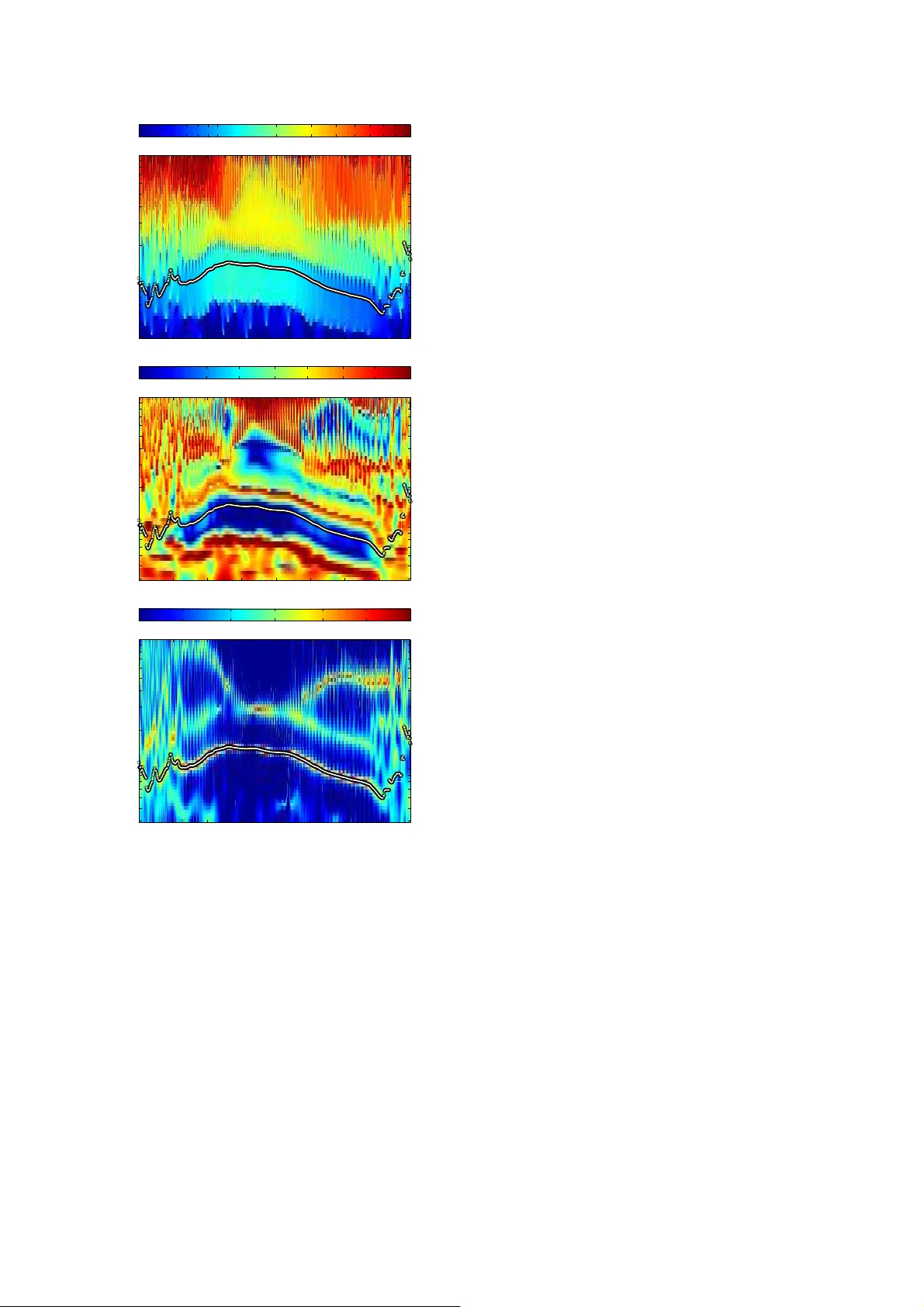
Using instantaneous fr equency and aperiodic ity detection to estimate F0 f or high-qu ality speech s ynthesis ∗ Hideki Kawahara 1 , 2 , Y annis Agiomyr giannakis 1 , Heiga Zen 1 1 G o o g l e 2 W akayama University , Japan kawahara@sys. wakayama-u.ac .jp, { agios,heiga zen } @google.com Abstract This paper introduces a general and fl exible framework for F0 and aperiodicity (additi ve non periodic compo nent) analy- sis, specifically intended for high-quality speech syn thesis and modification applications. The proposed frame w ork consists of three subsystems: instantaneous frequenc y estimator and initial aperiodicity detector , F0 trajectory track er , and F0 refinement and aperiodicity extractor . A preliminary implementation of the proposed frame work substantially outperformed (by a fac- tor of 10 in terms of RMS F 0 estimation error) existing F0 ex- tractors in tracking ability of t emporally v arying F0 trajecto- ries. The front end aperiodicity detector consists of a complex- v alued w av elet analy sis filter with a highly selectiv e t emporal and spectral en v elope . This front end ap eriodicity detector uses a ne w measure that quantifies the de viation from periodicity . The measure is less sens itiv e to sl o w FM and AM an d closely correlates with the signal to noise ratio. The front end com- bines instantaneo us frequency information ov er a set of fi lter outputs using the measure to yield an observation probability map. The second stage generates the initial F0 trajectory using this map and sign al po wer information. The final stage uses the de viation measure of each harmonic co mponent an d F0 ad ap- tiv e time warping to refine the F 0 esti mate and aperiodicity es- timation. The proposed framew ork is fl exible to integrate other sources of instantaneous frequen cy when they pro vide rele v ant information. Index T erms : fundamental frequenc y , speech analysis, speech synthesis, instantaneous frequenc y 1. Intr oduction This paper describes a ne w F0 track er for rapidly changing F0 trajectories with aperiodicity , which represents additive non- periodic compo nents. In high -quality speech synthe sis and modification applications [1–3], surpassing 4.2 o n the 5 point MOS score, glitches in aperiodicity handling and t he failure to follow rapidly changing fundamental frequencies (F 0) are harmful to processed spe ech quality . Introducing a generativ e model of F0 tr ajectory (for example [4]) to F0 estimation pro- vides well behav ed and parametric representation. Ho we ver , the estimated F0 trajectories are still not good enough for high- quality speech synthesis. The actual e xcitation signal of speech, glottal flo w , contains se veral sources of fluctuations [5] and c on- sequently , the observed F0 trajectories are differen t from the ∗ The original version wa s accepte d for presentation at 9th ISCA W orkshop on Speech Synthesis, CA USA, September 13th-15th 2016. trajectories produced by those models. T o attain highly natu- ral synthetic speech it is important to retain these fine temporal v ariation in F 0 trajectories [6, 7]. Although many F0 ex tractors hav e been proposed [8–12], in practice, parameter tuning and/or manual error correction is often necessary . In addition, their performance when extracting such fine temporal variations has not been in v estigated exp licitly . That is the goal of this paper . This paper is organized as follows. S ection 2 discusses the motiv at ion and tar get for de signing a new F0 obse rver , based on a revie w on existing issues. It also defines ape riodicity , which is relev ant for speech analysis and synthesis. Section 2.2 presents objecti ve measures used in this pap er . Based on these, se ction 3 introduces a general scalable architecture for F0 observ er . It consists o f three subsystems: front end aperiodicity detectors, the best trajectory finder , and F0 initial estimate and refinement subsystem with aperiodicity e xtractor . Sub-sections 3.1 and 3 . 3 introduce the front end and the refinement subsystems, respec- tiv ely . In section 4, these subsystems are e valuated using artifi- cial test signals. Section 5 d iscusses remaining issues. Example analysis results using actual spe ech samples an d mathematical details are giv en in appendices. 2. Backgr ound Speech synthesis requires dependab le F0 values whene ver pro- ducing voiced sounds. Howe ver , e ven for copy-synthesizing from actual sp eech samples, where the targets are known, this is not always easy , since voiced sounds are not purely periodic and defining F0 v alues for such signals is not a trivial issue . Figure 1 shows a beg i nning of a sentence from our speech corpus. From 0.2 s to 0.52 s, the speech signal is voiced. Ho w- e ver , due to irreg ularities in glottal vibrations, defining the F 0 is difficult. The lower plot shows the F 0 tracks by YIN [10] and SWIP E ′ [12] to illustrate the issues. It is difficult to ev al- uate the relev ance of these tracking results. Y et these two state of the art systems do not produ ce consistent results. The fact that voicing without vocal fold contact is not rare [13, 14] pre- vents using EGG (electroglottograph) for the source of ground truth. Using the extracted trajectory and comparing the synthe- sized speec h and the original speec h is a reasonable test b ut it is very demanding on human resource and time to obtain reliable results. An alternati ve approach for ev aluating F0 extractors is to use an objecti vely defined artificial test signal. The ideal can- didate is a speech signal, where the ground truth is av ai lable and provid es wide div ergence and variab ility . Instead, this -0.5 0 0.5 frequency (Hz) 0 200 400 600 800 1000 1200 1400 time (s) 0.15 0.2 0.25 0.3 0.35 0.4 0.45 frequency (Hz) 200 250 300 YIN SWIPE' Figure 1: Example of the d ifficulty of handling irregular voic- ing. Upper plot shows speech wav eform. Middle sho ws spec- trogram using 25 ms Blackman windo w with 1 ms frame shift. Lowe r plot shows F0 trajectories extracted using YIN and SWIPE ′ . Around 0.25 s to 0.3 s, deviation s caused discrep- ancies and/or failure of the baseline F0 trajectory track ers. article uses the excitation source signal defined by the L–F (Liljencrants–Fant) model [15]. The L–F model represents the time deri vati ve of t he glottal flow using a set of equations wit h four parameters. Ho wev er , directly digitizing the L–F model, which is defined in the continuous time domain, introduces spurious compone nts du e to aliasing. T o alleviate this aliasing problem this paper uses a closed-form representation of the anti- aliased L–F model defined in the continuous time domain [16]. Since the model is defined in the con tinuous time domain , it is easy to generate a sign al using a giv en F0 trajectory tha t will be the ground truth used in this paper . 1 [20–22] Figure 2 sho ws an examp le of F0 tracking using a sinu- soidally frequency modulated F0 tr ajectory as the test signal. This test sig nal has a vibrato of 16 Hz, wh ich is l arge compared to the normal human v oice, but demonstrates the problems due to rando m, cycle-by-cycle v ariations in the F0. The tested F0 extractors are YIN [10], SWIPE ′ [12], NDF [11], DIO [23] and the proposed method , which is described in Section 3. The tra- jectories obtained by YIN and SWIPE ′ are strongly distorted and attenuated, perhaps because the F0 is changing faster than these models allow . When these distorted trajectories are used to generate the excitation source for copy-syn thesis, t he out- put is perceiv ed differently . This is because the distortion adds fast-chang ing modulation comp onents that are not in the origi- nal signal. The ef fects of these spurious compo nents are made worse because humans are far more sensiti ve to fast frequency modulations than amplitude modulations [24, 25]. V oiced sounds are usually conside red as periodic, and to first approximation the glottal p ulses do occur at regular inter- v als. But due to prosodic needs the F0 of a voice is constantly changing, sometimes a simple glide as in the rise of F0 in a 1 In an open-sou rce imple m entat ion [17, 18] o f the anti-a liased L–F model [16], the m odel parameters can be cont rolled each glotta l cycl e indepen dently to si mulate the det ails of v ocal fol d beha viour [19]. It can be combined with a time varyi ng lattic e filt er to simulat e the dynamic speech producti on pro cess, whic h modulat es observed F0 through in- teract ion betwee n harmonic component and the group delay associated with resonanc es (formant trajecto ries). But these detai led simula tions are for further study . time (s) 0.58 0.6 0.62 0.64 0.66 0.68 0.7 frequency (Hz) 115 116 117 118 119 120 121 122 123 124 125 126 Trueth T 10 ° T 10 ° H 3 YIN SWIPE' NDF Dio Figure 2: Frequency modulated F0 t racking. Black thin line on top sho ws w av eform of t he L–F (Liljencrants–Fant) model [15, 16] output. T he very thick blue line sho ws the true F0 tra- jectory , which was used to generate the test signal. The refined F0 trajectory by the propo sed method (thick light green line) almost ov erlays on the true trajectory . question, and sometimes in a re gular fashion, as with vibrato. And, sometimes F0 varies in a more complex patterns, such as in tonal languag es, where the F0 trajectory con veys linguistic information. On top of these intended changes i n F0, there are modulations du e to physiolog ical aspects of voice production. The stocha stic nature of neural pulses which dri ve the muscles of t he vocal organ is a strong noise source and the critical con - ditions that produce vocal fold oscillation introduce bi-stable o r chaotic vocal fold vibration, especially during voice onset and of fset. Age related change and physical body status also affects the stability of vibration [5]. All these de viations from pure periodicity p lay important roles in speech communication and make speech a much richer media than text [26]. It is impo r tant to properly an alyse and replicate these d e- viations from periodicity in high-quality spe ech synthesis and modification applications. Accurately estimating aperiodicity is still a very challenging problem. Tracking errors introduces spurious compone nts [27, 28] and they add to the original ran- dom componen t. These are the reasons why F0 tracking dis- tortions as sho wn in F ig. 2 are harmful for high-quality speech synthesis. T wo issues have to be properly solv ed : accurate es- timate and tracking of changing F0 tr ajectory and a ccurate esti- mate of random compo nents based on the accurate esti mate of F0 trajectory . These issues moti vate us to de velop a framew ork that pro- vides a calibrated procedure t o describe the amount of aperiod- icity and to track F 0. The primary analysis targe t is high quality speech corpus recorded in a quiet and acoustically controlled en vironment using high - fidelity microphones. The aim here is to provide accurate, certifi ed metadata, in this case, F0 value and an inde x that represents the accuracy of the estimated F0 as well as a measure that represents t he amount of aperiodic- ity . Processing speed is not the first priority of the framew ork described here. Note that these metadata depend only on the data in the analysis frame, because there is no reliable model yet for the dynamic behavio ur of F0 and aperiodic compo- nent. Using models of dyna mic F0 beh aviou r such as Fujisak i’ s model [29], or F0 continuity constraint, may introduce biases due to model mismatch. Frame-based F0 with aperiodicity in- formation, which the propo sed system produce s, will help to establish certifiably accurate models of the statist ical/dynamic behav i our . 2.1. What is aperiodicity? For speech synthesis applications, amplitude and F0 are con- trollable parameters of the excitation source. Howe ver , only replicating amplitude and F0 precisely to the original speech yields poor quality synthetic sounds. An important attribute of excitation is missing. This missing attribute is aperiod i city . 2 In t his paper , attribu t es t hat can be r epresented by amplitude and F0 modulation are no t included in the definition of aperiod- icity . What is left after remo ving periodic component defines “aperiodicity” in this paper . It turns out that our system’ s F0 estimation error is well co r related with the system ’ s estimate of aperiodicity , described below . 2.2. Measures f or objectiv e evaluation F0 extractors hav e been e v aluated based on error-rate related measures; such as Gross Pitch Error (GPE), V oicing Detec- tion Err or (VDE) [ 30] and Pitch Tracking Error (P TE) [31]. Attaining high performance in these measures is a prerequi- site for good F0 ex tractors. In this paper , we focus on F0 tracking fidelity , because the proposed method does not make voiced /un voiced decision. Instead, this F0 t racker outputs a measure of aperiodicity , which closely correlates with t he stan- dard de viation o f the relativ e F0 estimation error from the true v alue. This aperiodicity detector also is an informativ e sou rce of the type of ex cit ation. The voice d/un voiced decision is left to the application, which can use the output of the proposed method to make this decision. 3. Ar chitectur e and subsystems The proposed framew ork, Y ANGSAF (Y et ANother Glott al Source Analysis F rame work), computes the instantaneous F0 using three steps: estimate, track, and refine. The estimation step calculates three features of the input signal ov er a num ber of ban dpass channels. The maximum fr om the estimate stage is then tracked to p r oduce a local estimate of the F0. Finally , an optional refinement stage combines temporal and harmonic information to produce a more accurate estimate of F0. 3.1. Estimation The first stage of the Y ANGSAF algorithm analyses the signal with a number of band pass ch annels, and then estimates three v alues for each channel as a function of time. These values are 1) the local instantaneo us frequency , 2) a measure called ape- riodicity that represents the amoun t of variability in the chan- nel’ s frequ ency estimate, and 3) a probab i listic estimate that the channel contains a good representation of the F0. These sig- nals are described in the subsections that follo w and are used in the tracking stage described by Section 4.2. Figure 3 sho ws a diagram of the estimating detector in each channel. The front end breaks the input into a numb er of spectral 2 Effe cts of spectral en velope are also ignored. These detail s e xceed the scope of this paper . 1 | . | | . | 2 X 1 | . | X + + - Flanagan's equation Figure 3: S chematic diagram of aperiodicity detector . Upper part calculates instantaneous fr equenc y using Flanagan’ s equa- tion (Appendix A). The lo wer part calculates aperiodicity mea- sure as a relativ e residual leve l a ks (Appendix B). channels using a bank of bandpass filters, each centered at f c . 3 The ce nter freq uencies co ver the possible F0 ran ge, with a fixed separation on the logarithmic f requenc y axis. The current im- plementation co vers 400 Hz to 100 0 Hz using 12 channels and detectors in each octav e. The i nstantaneous frequen cy estimate needs both the complex - v alued si gnal and its deri vati ve. These values are cal- culated starting wi th bandpass filter h ( τ , f c ) and its deri vati ve h d ( τ , f c ) shown in F ig. 3 and desc ribed in Appen dix A. Each bandpass fi lter has linear ph ase, is a zero-delay FIR filter, has a comple x-valued response, and passes only the positive f re- quenc y compon ents. Figure 4 sho ws an example of these three estimated signals for a sequence of vo wels. 3.1.1. Instantaneous F reque ncy The instantaneous frequenc y of the si gnal contained within each channel is calculated using Flanagsn’ s approach, which is based on the logarithm of a comp lex signal x ( t ) and its deri va- tiv e. An AM/FM modulated signal is represented in polar form x ( t ) = r ( t ) e j θ ( t ) . The i nstantaneous (angular) frequenc y ω i ( t ) is defined as the de riv ativ e of the phase c omponen t θ ( t ) , namely ω i ( t ) = dθ ( t ) dt . The instantane ous frequenc y can be derived by starting with the logarithm of the componen t phase and using a bit of algebra: d log( x ( t )) dt = d log  r ( t ) e j θ ( t )  dt = d log ( r ( t )) dt + j dθ ( t ) dt (1) ω i ( t ) = ℜ [ x ( t )] d ℑ [ x ( t )] dt − ℑ [ x ( t )] d ℜ [ x ( t )] dt | x ( t ) | 2 , (2) where ℜ [ x ] and ℑ [ x ] represents the real and the imaginary part of x , respecti vely . The deriv ation o f this expression is c ontained in Appendix A. 3.1.2. Aperiodicity W e also wish to calculate a measure of the aperiod icity of the signal in each chann el, which will be used as a measure of the reliability of the instantaneou s frequenc y measurement. For a constant sinuso id, the aperiodicity is zero, and the aperiodicity gro ws as the signal v aries (wigg les) more within the bandpass 3 The -3 dB points in frequenc y are 0 . 745 f c and 1 . 255 f c . The zero points are l ocated at 0 and 2 f c . The -3 dB p oints in time are − 0 . 456 /f c and 0 . 456 f c . Support is ( − 2 /f c , 2 /f c ) . instantaneous frequency map of /aiueo/ filter center frequency (Hz) time (s) 0 0.1 0.2 0.3 0.4 0.5 0.6 0.7 40 50 70 100 200 300 500 700 900 40 50 70 100 200 300 500 700 900 aperiodicity map of /aiueo/ filter center frequency (Hz) time (s) 0 0.1 0.2 0.3 0.4 0.5 0.6 0.7 40 50 70 100 200 300 500 700 900 0.0001 0.0003 0.001 0.003 0.01 0.03 0.1 0.3 1 probability map of /aiueo/ filter center frequency (Hz) time (s) 0 0.1 0.2 0.3 0.4 0.5 0.6 0.7 40 50 70 100 200 300 500 700 900 0.001 0.003 0.01 0.03 0.1 0.3 Figure 4: Example of the first stage detector ou t puts. The up - per plot sho ws the instantaneo us frequency map. The middle plot sho ws the residual map. The bottom plot sho ws t he prob- ability map. T he speech material is a Japanese vo wel sequence /aiueo/ spoken by a male. For reference purpose , the F0 trajec- tory extracted in the third stage is overlaid using open circles. In the p r obability map, the periodic vertical lines are sy nchronized with vocal fo ld vibration. The upper right trace of periodicity corresponds to the response of first formant of vo wel /o/. channel. The basic idea of the periodicity detector is to calculate the amount of energy in the band-passed signal t hat is not the primary sinusoid. The primary sinusoidal compon ent will hav e the largest ener gy , and when the complex signal is normalized to hav e unit magnitude, refiltered, and then r enormalized, the primary sinuso id will still have unit magnitude. The other com- ponents will b e filtered with a non - unit gain, since the filter is not an ideal brick-wall filter , and their amplitude will ch ange. Subtracting the original an d the twice-filtered and normalized response gi ves an estimate of the aperiodicity . Note this es ti- mate is done without ex pli citly identifying the primary sinusoid and its frequenc y . When a signal x whose fundamental frequency is equal to f c is filtered, only the fundamental comp onent, a complex- v alued, slo wly time-varying signal, is passed (appears in y 1 ) and is normalized to become y ′ 1 . Then, by using the same filter , filtering signal y ′ 1 again, and normalizing the ov erall amplitude using t he absolute v alue of the c omplex valued-signa l, the twice filtered (and amplitude normalized) signal y ′ 2 is obtained. Sub- tracting this twice filtered and amplitude normalized signal y ′ 2 from the amplitude normalized fi rst filter output y ′ 1 , yields a residual signal r . Since the signal y ′ 1 is normalized , the power of t he residual represents the relative le vel of the other compo- nent(s). The difference between y ′ 1 and y ′ 2 corresponds to spectral componen t s in the chann el t hat are not the primary sinusoid. Calculating the energy in this signal ( a k ) , and smoothing it gi ves a ks which is this system’ s measure of harmonic aperi- odicity . Appendix B describes the relati on between t he SNR of t he original signal and the residual aperiodicity po wer using equations and examples. Placing band pass filters ha ving the same shape on the loga- rithmic frequenc y axis yields the detector to output higher ap eri- odicity value , when f c is located at harmonic frequen cies other than the fundamental. This is similar to the concept “funda- mentalness, ” which is explained in Fig. 11 of reference [32]. Appendix sho ws relation between filter shape examples and har- monic compon ents. The instantaneous frequency calculation and the aperiodic- ity calculation yield v alues at the audio sampling rate. These audio sampling rate time series are do wn-sampled for later pro- cessing. In this work the down-sam pling is accomplished by extracting the nearest ti me samples from each time series, pro- viding two sequences of instan taneous frequency and aperiod - icity measure v alues at the frame rate (i.e. 200 Hz). 3.1.3. Prob ability The fundamen tal co mponent in the original signal is dominant in a numb er of ou t put channels because there is little else for fil- ters centered at frequ encies lo w er tha n th e se cond h armonic can respond. Thus a numb er of channels will respond in the sam e way to th e fundamental componen t , as seen by the blueish blob around 100Hz in the second panel of Fi gure 4. All chann els inside this blob ha ve information about the fundamental com- ponent, but with dif ferent reliabilities. Giv en a numbe r of (distinct) estimates of the true F0, all from dif ferent channels, a probability map indicates which channel will hav e the best estimate. T o create this probabil- ity map, all the instantaneous frequ ency and aperiodicity esti- mates are con verted into Gaussian probability masses ce ntered at va rious instantaneous frequency estimates. The output of the channel’ s ap eriodicity estimate ( a ks , a measure o f smoothed en- ergy) is co n verted into a v ariance σ 2 k by scaling. The scaling coef fi cient was empirically determined by a set of simulations. On a log-frequenc y scale ν , this gi ves a number of (indepen- dent) estimates of the instantaneous frequ ency , each modelled as a Gaussian mass centered at log ( f k ) , and with a v ariance of σ 2 k . Summing all these yields a probability density f unction p G ( ν ) r epresented as a Gaussian mixture. For each channel, integrating this distribution pro vides an observ ation proba bility P r [ k ] that chann el k should see the fundamental compon ent in its nominal pass band [ f L ( k ) , f H ( k )] is p G ( ν ) = N X n =1 ˆ b n √ 2 π σ 2 n exp  − (log( f n ) − ν ) 2 σ 2 n  (3) P r [ k ] = Z log( f H [ k ] ) log( f L [ k ] ) p G ( ν ) dν (4) f L [ k ] = f c [ k ]2 − 1 2 K , f H [ k ] = f c [ k ]2 1 2 K , (5) where K represents t he number of filters per octav e. This inte grates the instantaneous frequenc y probability dis- tributions between the frequency limits of fil ter k to arriv e at an estimate of ho w reasonable it is for channel k to provide an estimate of the F0. An e xample of this resu l t is sh o wn in the bottom of Figure4. 3.2. T rackin g Giv en the three instantaneou s maps (as a function o f frame time and spectral cha nnel) computed in Section 3.1, an initial esti- mate of the single best F0 at each frame is calculated by findin g the channel with the highest probability . This i s done in fou r steps: estimate the pitch range for this utterance, smooth the probability map, find t he highest probability F0, and the n refine the F0 esti mate. The result i s a smooth esti mate of the true F0 based on t he instantaneous frequ ency calculated in each chan- nel. First, the F0 search range is estimated by a weighted av er- age of the instantaneous frequencies seen in the utterance. The temporal weighting is calculated from the energ y in the orig- inal signal, after fil tering it between 40-10 00Hz, which is the prospecti ve pitch range. Then each frame of the instantaneous frequenc y map is weighted and combined to form an overall in- stantaneous frequency histogram. By weighting by the signal’ s amplitude at each point in time, the high-energ y portion of the utterance (vo wels) are treated with more importance. The median of this instantaneous frequenc y distribution (marginal distrib ution) defines the center point of the F0 search range. The tr acker looks for peaks in the probability distri bu- tion w ithin 1.2 octav es abov e this center point, and 1.3 octav es belo w , a total of a 2 .5 octav e range. Second, in order to better estimate the F0 at the start and end of voicing the probability map co mputed in Section 3.1 .3 is smoothe d in time using a 45ms Hanning windo w with am- plitude weighting. Smoothing is done before tracking so that we extend the F0 estimates at the start and end of vo i ced seg- ments. For e xample, at the onset of voicing, the probability at F0 i s not high, because the signal le vel i s l o w and t he SNR is lo w . Smoothing using amplitude weighting increases the prob- ability at F 0, because at frames after the onset the le vel grows and conse quently the SNR become higher . In other words, the probability distribution o f the onset frames become more lik e the p r obability distr ibution of later frames. This way smoothing reduces tracking error at the beginn i ng of voicing. The same thing happen s at the v oice offset. Thirdly , gi ven the F0 range and the smoothed probability map the best ch annel across time can be tracked. For a range of channels that are within the 2.5 octave range defined for the entire u tterance, and 0.7 octaves of the last fr ames best chan nel, the channel with the highest smoothed probability is chosen. Finally , this channel selection is further refined by returning to the original probability map computed in S ection 3.1.3 and choosing the channel with the highest probability closest to that bin chosen from the smoothed e stimate. The following provides the initial F0 estimate f O I . f O I = X m ∈ V [ k ] b m f m (6) V [ k ] = { m | 0 . 5 f c [ k ] < f c [ m ] < 1 . 25 f c [ k ] } , (7 ) where the best weights b m are calculated from σ 2 m in V [ k ] . 3.3. Refin ement of the initial estimate The third stage further improv es this F0 estimate by a dding tw o refinements. First, and most importantly , the higher harmonics of an F0 estimate can refine the estimate. Secondly , adaptiv e time warping of the origin al si gnal, com bined with further re- finement using higher harmo nics of the warped signal, reduces the amount of F0 trajectory de viation for better analyses. The first procedu r e uses harmonic frequencies and their v ari ance. Each harmonic compon ent, fr om first to m - th, has correspondin g aperiodicity detector . Each b andpass filter of th e detector has the same shape on the l inear frequency axis and does not cover neighbouring harmonic co mponents. Each de- tector yields instantaneous frequency f k and its aperiodicity a k , where k represents the harmonic number . T hese v alues are con verted to F0 estimate f k /k and its v ariance σ 2 k . The weighted averag e P m k =1 b k f k /k prov i des the refi ned F0 esti- mate. V ari ance values { σ 2 k } m k =1 are used to calculate the best mixing weights { b k } m k =1 (Appendix D). Ho wever , this refinement does not properly mak e use of higher harmonic information when the F0 trajectory i s rapidly changing. This is because a rapid movem ent of higher frequen- cies generates strong side-band compon ents and they smear the analysed harmonic structure [27, 28, 33]. Thus, the second procedure uses F0 adapti ve time axis warping to allev i ate this prob l em. Stretching the time axis, pro- portional to an instan t aneous F0 v alue makes t he observed F0 v alue constant [27, 28, 33] and keeps the harmonic structure in- tact. Then, placing aperiodicity detectors on harmonic frequen- cies, from first to m -th, th e weighted average o f F0 information yields the F0 estimate on the w arped time axis. Con verting this estimate value to th e value on the original time axis provide s the further improv ed F0 estimate. These t wo procedures are applied serially as well as recur- siv ely . Let H m represent t he op erati on o f harmonic based re- finement using the fi rst through m -th harmonic comp onents and T m represent the operation of F0 adaptiv e time warp ing-based refinement using the first through m -th harmonic components. Let P X [ x ; Θ] represent the function of initial estimate F0 where x r epresents the input signal and Θ represents a set of the asso- ciated design parameters for analysis. The following equations describes the configurations of the two tracke rs tested: H 10 ◦ H 3 ◦ P X [ x ; Θ] (8) T 10 ◦ T 10 ◦ H 3 ◦ P X [ x ; Θ] , (9) where T ◦ H represents the composite function of the function s T and H . Finally , by placing aperiodicity detectors on all harmonic frequencies in the warped t ime axis, estimated SNR around each harmonic component provides the excitation source information for speech synthesis. Because any F0 trajectories on this warped time axis are constan t in time, aperiodicity values which detec- tors output are consisten t with the a periodicity definition of t his paper . 4. Evaluation using test signals This paper uses two measures of performanc e. Most impor - tantly , the standard deviation of the relative error tells us the total dist ortion of the estimated F0 t rajectory from the ground truth. The second performance measure is the frequenc y- modulation amplitude tr ansfer function (FMTF ), which ex- presses ho w well a F0 tracker follo ws fast F0 modu lations. The test signal uses sinusoidal modulation on the logarithmic fre- quenc y axis, since F0 dynamics is better described on the log- arithmic fr equenc y axis [29]. Consequ ently , both FMTF and distortion ev aluation measures use l ogarithmic frequency to cal- culate their v alue. The proposed algorithms are i mplemented using M A T L A B and tested using synthetic signals. Only representati ve results are d escribed below . In the f ollo w ing tests, t he test signa ls were generated using the aliasing-free L–F model [16]. 4 The sam- pling frequency f s was 22050 Hz and the “mod al” v oice q uality parameters [34] for the L–F model were used in the follo wing examp les. W e t est this ne w F0 tracker in two different ways: additiv e noise and FM modulation. 4.1. Add itive n oise Firstly , the quality of the F0 estimate in t he face of additiv e white noise was tested usin g the configuration giv en by Eq. 8 ( H 10 ◦ H 3 ). The F0 extractor for the init ial esti mate (S ec- tion 3.2) ( P X [ x ; Θ] ) was tested to clarify the ef fects of r efine- ment (Section 3.3 ). Four popular F0 ex tractors were also ev al- uated f or reference; YIN [10], SWIP E ′ [12], NDF [11] and DIO [23, 35]. The y were tested using their default or recom- mended settings. A constant F0 trajectory was used in this test. Figure 5 shows the results for a 120 Hz F0. T he vertical axis represents the relati ve RMS error . W hen the SNR is larger th an 5 dB, YIN yielded the best results. But, YIN’ s performance is obtained at t he cost of poor temporal resolution, which will be sho wn in the follo wing test. DIO was designed for high -quality recordings and i s not tolerant to noise. While SWIPE ′ sho wed good performance from 0 to 20 dB SNR, performa nce saturated there after . The harmonic refinement procedure reduced the er- ror in the initial estimate by a factor of 8, ev en in high noise, because the standard dev iation of error in n -th harmon i c com- ponent i s 1 /n as described in previou s paragraph. In total, this is the second best result. 4 The original L-F model [15] is an ti-ali ased using a closed fo rm rep- resenta tion. T he M AT L A B implementat ion of this func tion and GUI- based interacti ve applicati on for speech scien ce education are open source [17 , 18]. Spuriou s lev els around the fundamental component of the model’ s output are lowe r than -120 dB. SNR (dB) -5 0 5 10 15 20 25 30 35 40 error SD (%) 10 -3 10 -2 10 -1 10 0 10 1 F0: 120 Hz H 10 ° H 3 P x YIN SWIPE' NDF DIO Figure 5: RMS error of F0 estimation vs. additiv e noise SNR for a t emporally cons tant F0. The initial estimate (tr iangle) er- ror de viations were reduced by a factor of 8 (circl e) by using harmonic refinement. modulation frequency (Hz) 10 0 10 1 gain (dB) -25 -20 -15 -10 -5 0 F0: 120 Hz T 10 ° T 10 ° H 3 H 10 ° H 3 Yin SWIPE' NDF DIO Figure 6: Frequenc y mo dulation transfer function for F 0 mod- ulation. The higher tracking frequency limit of the initial F0 estimate (triangle) is e xpanded two times by the propose d re- finement using F0 adapti ve time warping (circle). 4.2. Frequency modulation of F0 Measuring the ability of a F0 tracker to follo w F0 mo dulation is a more rel e vant test for speech sounds wit h rapid changes. The instantaneous frequenc y of the aliasing-free L–F model output was controlled at audio sampling rate (22050 Hz) resolution. The average F0 was 120 Hz wi th 100 musical cent p eak-to-peak modulation depth roughly to 6% frequenc y modulation peak-to- peak in frequency . 5 In t he t wo tests described i n this section, a bit of white noise (SNR 100 dB) was added . Figure 6 sho ws the frequency modulation transfer function for the four F0 t rackers that serv e as a benchmark and two v ari- ations of t he F0 track er described in this pap er. For v ery low vibrato frequency (low modulation frequenc y) all F0 trackers work well at high SNR. At higher modulation frequencies all F0 t rackers ex cept for T 10 ◦ T 10 ◦ H 3 fail to follow the full modulation, which shows up as a reduced gain when consid- 5 T ested F0 were 120, 240, 480 and 800 Hz. For F0 extracto rs, 120 Hz is the worst cond ition in terms of tracking. modulation frequency (Hz) 10 0 10 1 F0 error SD (%) 10 -4 10 -3 10 -2 10 -1 10 0 F0: 120 Hz T 10 ° T 10 ° H 3 H 10 ° H 3 Yin SWIPE' NDF DIO best 1 ms best 5 ms Figure 7: RMS err or of F0 trajectory tracking. T he RMS error of the refined F0 trajectory using harmonic fr equencies (trian- gle) is reduced by a factor of 10 or more by introducing F 0 adapti ve time warping (circle). ering the outpu t vs input modulation deviation. For higher F0 signals, the 3 dB point increased prop orti onally to the F0 v alue, excep t YIN. Figure 7 sho ws the RMS error of the F0 trajectories as a function of the modulation freq uency . The dashed line and dash dot line show the RMS error of the best app r oximation to the true F0 using piece-wise linea r function wi th segment lengths 1 ms and 5 ms respecti vely . SWIPE ′ and YIN y ielded lar ge RM S error, corresponding to the strong distortion shown in Fi g. 2. The refinement per- formance without time warping is comparable to NDF . DIO sho wed the best performance amon g popular methods. The re- fined F 0 t rajectory using F0 adapti ve time warping reduces the RMS error by a facto r of 10 or more o ver the range from 2 Hz to 16 Hz modulation. For higher F0 values, RMS errors of other methods decrease in versely proportionally to the F0 va lue. The F0 adapti ve ti me warping also reduced spurious com- ponent due to FM substantially . For example, for a test sig- nal with 16 Hz frequency modulation and 100 musical cent p-p depth, the refined F0 by the analysis configuration T 10 ◦ T 10 ◦ H 3 reduced spurious residual le vels lower than − 40 dB. This is p er- ceptually negligible. 5. Discussion The goal of this paper is to estimate F0 trajectories, which con- sist of rapidly changing components, acc urately for high-quality speech synthesis. The proposed set of procedures provide a prospecti ve frame work. Howe ver , the follo wing aspects of F0 estimation were not exploited here. In vestigations of the fo llow- ing issues could be important for improving synthesis quality further . Plosiv e so unds such as /k/, /t/ sometimes sound like fri ca- tiv e by smea ring tempo r al sharpn ess due to the smoothing ef- fect of time windo wing. This i s a com mon degradation fou nd in STRAIGHT . Some speakers and langu ages frequen tly use “creaky voice. ” Representing these sounds using periodic signal plus noise results in poor reproduc tion. Rel e vant analysis and repre- sentations hav e t o be in vestigated. T emporal v ariation of F0 consists of effec ts caused by in- teractions between harmonic compone nts and group delay in vocal tract transfer function. It is desirable to compensate this effe ct for speech synthesis applications, because this effect can be accumulated in each analysis and synthesis cycle. In addition, it is interesting to consider a unique F0 tracker based on Harmonic-Lock ed Loop tracking [36] as an alterna- tiv e F0 refinement procedure for the third stage of t he proposed frame work. 6. Conclusions This paper introduced a framew ork for intantaneous estimates F0 and aperiodicity . It is able to impro ve the ability of F0 ex- tractors to temporally follow v arying F0 trajectories by a factor of 10. It may serve as an useful infrastructure for speech re- search and applications. 7. Ackno wledgements The authors appreciate insightful discussions with Prof. Ro y Patterson on hu man auditory perception, especially on fine tem- poral structure and detection of interfering sounds. Malcolm Slaney provided ed i torial assistance . He an d Dan Elli s also pro- vided producti ve as well as critical comments. A. Note on the Flanagan’ s equation Flanagan use s the time deri vativ e of the log ari thm of a complex signal x ( t ) to estimate the instantaneous frequency . By intro- ducing a logarithmic function, the phas e compone nt is linearly separable from amplitude. log( x ( t )) = log( r ( t ) exp( j θ ( t ))) = log( r ( t )) + j θ ( t ) (10 ) ℑ [log( x ( t ))] = θ ( t ) . (11) T o make deri vation simpler , as far as no ambiguity is intro- duced, time dependency representation by ( t ) is omitted after- wards. ω i = dθ dt = ℑ  d log ( x ) dt  = ℑ  1 x dx dt  = ℑ " da dt + j db dt a + j b # where x = a + j b = ℑ "  da dt + j db dt  ( a − j b ) ( a + j b )( a − j b ) # = ℑ " a  da dt + j db dt  − j b  da dt + j db dt  a 2 + b 2 # = ℑ " a da dt + j a db dt − j b da dt − b db dt a 2 + b 2 # = a db dt − b da dt a 2 + b 2 = ℜ [ x ] d ℑ [ x ] dt − ℑ [ x ] d ℜ [ x ] dt | x | 2 . (12) Which is the Flanagan’ s equation. The complex-v alued signa l x in Eq. 12 is a filtered o utput of h ( t ) . It is a function of the center frequency f c and time. Let e xplicitl y represent x using X ( ω c , t ) and its time deriv ativ e using X d ( ω c , t ) . Then the follo wing holds. X ( t, ω c ) = Z ∞ −∞ h ( λ ) x ( t − λ ) dλ = − Z ∞ −∞ w ( τ − t ) exp ( j ω c ( τ − t )) x ( τ ) d τ (13) X d ( t, ω c ) = dX ( t, ω c ) dt = − d dt  Z ∞ −∞ w ( τ − t ) ex p ( j ω c ( τ − t )) x ( τ ) dτ  = − Z ∞ −∞  − d w ( τ − t ) dt − j ω c w ( τ − t )  · exp ( j ω c ( τ − t )) x ( τ ) d τ = Z ∞ −∞ h d ( λ ) x ( t − λ ) dλ, (14) where w d ( t ) = dw ( t ) dt + j ω c w ( t ) (15) h d ( t ) = w d ( t ) exp( j ω c t ) . (16) Substituting these two time wi ndo ws w ( t ) and w d ( t ) into Eq. 12 remov es ti me deri v atives: ω i ( t, ω c ) = ℜ [ X ( t, ω c )] ℑ [ X d ( t, ω c )] − ℑ [ X ( t , ω c )] ℜ [ X d ( t, ω c )] | X ( t, ω c ) | 2 , (17) Note t hat the TKEO (T eager Kaiser E nergy Operator [37]) is not relev ant for estimating rapidly changing F0 trajectories, since it uses an approximation, which requires slowly chang- ing AM and FM. Using Flanagan’ s equation is rele van t, since it does not rely on this approximation. B. Residual calculation in each detec tor This section sho ws how the aperiodicity detector in F ig. 3 works. The input to this detector is x ( t ) . Let h ( t, f c ) repre- sent the complex valued impulse response of each band pass filter centered around f c . a k ( t, f c ) = | r ( t, f c ) | 2 (18) r ( t, f c ) = y ′ 1 ( t, f c ) − y ′ 2 ( t, f c ) (19) y ′ 2 ( t, f c ) = y 2 ( t, f c ) | y 2 ( t, f c ) | (20) y 2 ( t, f c ) = Z 2 /f c − 2 /f c h ( τ , f c ) y ′ 1 ( t − τ ) d τ (21) y ′ 1 ( t, f c ) = y 1 ( t, f c ) | y 1 ( t, f c ) | (22) y 1 ( t, f c ) = Z 2 /f c − 2 /f c h ( τ , f c ) x ( t − τ ) dτ , (23) where the integration interval ( − 2 /f c , 2 /f c ) is for the Nut- tall windo w (Eq. 25). For Hann windo w the interval i s ( − 1 /f c , 1 /f c ) and for B lackman window the interval is ( − 1 . 5 /f c , 1 . 5 /f c ) . Band pass filters having these impulse re- sponse lengths hav e fi rst spectral zeros at 0 and 2 f c . Smoothing the relativ e residual lev el a k ( t, f c ) yields the aperiodicity parameter a ks ( t, f c ) . a ks ( t, f c ) = Z 2 /f c − 2 /f c | h ( τ , f c ) | a k ( t − τ , f c ) dτ . (24) signal location (re. center) 0 0.5 1 1.5 2 gain (dB) -50 -40 -30 -20 -10 0 10 filter filter 2 residual filter signal location signal location (re. center) 0 0.5 1 1.5 2 relative residual (dB) -60 -50 -40 -30 -20 -10 0 40 dB 30 dB 20 dB 10 dB 0 dB -10 dB Figure 8: principles of operation. Upper plot sho ws filter shape and the dominant signal at 1 . 14 f c . Fil ter gains are adjusted to make outpu t lev els are 0 dB. Subtracting the second fi lter gain from the first one yields the equi valent filter for other compo- nents. Lo wer plot sho ws the output residual level as a function of the location of the dominant signal and the noise le vel. B.1. Operation and implementation of the procedure Figure 8 illustrates the process use to calculate the aperiodicity componen t . The impulse respon se of the filt er h ( t, f c ) is w ( t ) = 3 X k =0 a k cos(2 π k f c t ) | t | < 2 f c (25) h ( t, f c ) = w ( t ) exp(2 π j f c t ) , (26) where j = √ − 1 and t he coefficients { a k } 3 k =0 are (0.338946, 0.481973 , 0.1610 54, 0.018027). This is the 11-th item in T able II of Nuttall’ s work [38]. 6 The detector is design ed to cancel the primary periodic componen t in the input signal by adjusting the fi lter gain at the frequenc y of the primary componen t. This is done by normal- izing the output by its RMS le vel. In a high SNR case, to- tal RMS le vel of the filt ered signals are approximately equal to the RMS le vel of the period ic componen t . The RMS leve l of the lower level compo nents are af fected by this suppression process. Since the equiv alent filter gain from this su ppression process is the difference of t wo fi lters, it yields the filter shape 6 In terms of time-freq uenc y product, when both is bounded, plorate spheroida l wa ve function is theoretica lly the best [39, 40]. Howe ver , due to large spe ctral dynamic range of actua l speec h signals, cosine series wi ndows, which ha ve v ery lo w side lobe lev el and stee p side lobe decay [38] yielded better performance . 10 1 10 2 10 3 0 0.1 0.2 0.3 0.4 0.5 0.6 0.7 0.8 0.9 1 frequency (Hz) gain (absolute value) aperiodicity detector for front end detector at 100Hz 2nd filter residual gain detector at 500Hz 2nd filter residual gain harmonics of 100 Hz 0 100 200 300 400 500 600 0 0.1 0.2 0.3 0.4 0.5 0.6 0.7 0.8 0.9 1 frequency (Hz) gain (absolute value) aperiodicity detector for refinement detector at 100Hz 2nd filter residual gain detector at 500Hz 2nd filter residual gain harmonics of 100 Hz Figure 9: Detector allocation of the front end (up per plot) and the refinement stage (lo wer plot). sho wn in the red curve of left plot of Fig. 8. The right p l ot of Fig. 8 sho ws the output aperiodicity parameter a k as a function of the loca tion of the primary component and the le vel of the lo wer lev el components. C. Detector allocation Figure 9 shows detector filter shapes of front end and the third stage. In the front end, the filter width is proportional to the center frequency . In the r efinement stage, the filt er width is constant. The filters in the refinement stage are designed using the estimated F0. D. Mixing F0 information The ban d of estimators in the front end indepen dently esti mate instantaneous frequenc y and an estimate of the quality of this estimate in the form of an aperiodicity measure. W e need to consolidate these estimates to get a single estimate of F 0 and we do this with a weighted av erage. Assume a set of random v ariables X k , k = 1 , . . . , N hav- ing zero mean ( E [ X k ] = 0 ) and v ariances σ 2 k ( V ar[ X k ] = σ 2 k ). W e wish to gene rate a new estimate from all the noisy estimates by weighting the individual estimates to arrive at an answe r with the minimum estimated variance. Thus, assume the follo wing cost function. L = V ar " N X k =1 b k X k # , (27) where b k represents the mixing coef ficient. When mixing F0 estimates deri ved from different sources, t he sum of weights has to satisfy the condition ( P N k =1 b k = 1 ). The optimum coef ficients ˆ b k for k = 1 , . . . , N − 1 are deri ved by solving the follo wing set of equations. σ 2 N = b k σ 2 k + σ 2 N N − 1 X n =1 b n for ( k = 1 , . . . , N − 1) . (28) The final coef ficient ˆ b N is giv en by ˆ b N = 1 − N − 1 X k =1 ˆ b k . (29) Other source of F0 in formation can be u sed to i mprov e this estimate further , if the variance of the estimate is av ailable. E. Refer ences [1] Z. Heiga, T . T omoki, M. Nakamura, an d K. T okuda, “Details of the Nitech HMM-based speech synthesis system for the Blizza rd Challe nge 2005, ” IEICE transactions on information and systems , vol. 90, no. 1, pp. 325– 333, 2007. [2] H. Ka wahara, M. Morise, Banno, and V . G. Skuk, “T emporally v ariabl e multi-a spect N-way morphing based on inter ference -free speech represen tations, ” in ASPIP A ASC 2013 , 2013, p. 0S28.02. [3] Y . Agiomyrgianna kis, “V OCAINE the voc oder and app licat ions in speech synthesis, ” in ICASSP 2015 , 2015, pp. 4230–4234. [4] H. Kameoka, K. Y oshizato, T . Ishihara, K. Kado waki, Y . Ohishi, and K. Kashino, “Generat i ve modeling of voice fundamental fre- quenc y contours, ” IEEE T rans. Audio, Speech, and Language Pro- cessing , vol. 23, no. 6, pp. 1042– 1053, 2015. [5] I. R. Ti tze, Principles of voice pr oduction . National Cente r for V oice and Speech, 2000. [6] T . Saitou, M. Unoki, and M. Akagi, “Dev elopment of an F0 con- trol model based on F0 dynamic character istics for singing-voi ce synthesis, ” Speec h commu nicati on , vol. 46, no. 3, pp. 405–417, 2005. [7] L. Ardaill on, G. De gotte x, and A. Roebel, “ A multi-la yer F0 model for singing voic e synthesis using a B-spline representat ion with intuiti ve controls, ” in Interspeec h 2015 , 2015. [8] P . Boe rsm a, “ Accurate short-t erm analysis of th e funda m ental fre- quenc y and the harmoni cs-to-noi se ratio of a sampled sound, ” in Pr oceedi ngs of the institute of phonetic sciences , v ol. 17, no. 1193. Amsterdam, 1993, pp. 97–110. [9] D. T alkin, “ A ro bust algorit hm for pitch trackin g (RAPT), ” Spee ch coding and synthesis , vol. 495, p. 518, 1995. [10] A. de Che vengn ´ e and H. Kaw ahara, “YIN, a fundamenta l fre- quenc y estimator fo r speech and music, ” JASA , vol. 111, no. 4, pp. 1917–1930, 2002. [11] H. Kawaha ra, A. de Che veign´ e, H. Banno, T . T akahashi, and T . Iri no, “Nearl y defect-fre e F0 t rajectory extracti on for expres- si ve speech m odificat ions based on STRAIGHT .” in Interspeec h 2005 , 2005, pp. 537–540. [12] A. Camacho and J. G. Harris, “A sawtoo th wa vefo rm inspi red pitch estimator for speech and music, ” JASA , vol. 124, no. 3, pp. 1638–1652, 2008. [13] D. Ch ilders, D. H icks, G. Moore, and Y . Alsaka, “ A model for voca l fold vibratory motion, contac t area, and the electrog lot- togram, ” JASA , vol . 80, no. 5, pp. 1309–1320, 1986. [14] D. H. Klat t and L . C. Klatt, “Analy sis, synthesis, and perception of v oice qual ity v ariati ons among fe male and male talk ers, ” JASA , vol. 87, no. 2, pp. 820– 857, 1990. [15] G. Fant, J. L iljenc rants, a nd Q. Lin, “A four-pa rameter model of glotta l flow, ” Speec h T rans. Lab . Q. Rep., Royal Inst. of T ec h. , vol. 4, pp. 1–13, 1985. [16] H. Ka wahara, K.-I. Sakakibara, H. Banno, M. Morise, T . T oda, and T . Irino, “Aliasing-f ree implementati on of discrete-time glot- tal source models and thei r ap plica tions to speech synthesis and F0 extra ctor ev aluation, ” in APSIP A 2015 , Hong K ong, 2015. [17] H. Kaw ahara. (2015) SparkNG: MA TL AB realtime re- search tool s for speech scienc e educa tion. [Online]. A vaila ble: http:/ /www . sys.wakayama - u.ac.jp/%7ekawa hara/MatlabRealtimeSpeechT ools/ [18] ——, “SparkNG: Interacti ve MA TLAB tools for int roduction t o speech production, per cepti on and processing fundamentals an d applic ation of the aliasing-fr ee L -F model component, ” in Inter- speec h 2016 . ISCA, 2016, p. Sho w and T ell, (Accepted). [19] K.-I. Sakakibar a, H. Imagaw a, H. Y okonish i, M. Kimura, and N. T ayama, “Physiological observa tions and synthesis of subhar- monic voice s, ” in AP SIP A ASC 201 1 , 2011, pp. 1079–1085. [20] G. Fa nt, “The LF-model re visited. Transfor mations a nd frequenc y domain analysis, ” Speec h T rans. Lab. Q. Rep., Roya l Inst. of T ech. , vol. 2-3, pp. 121 –156, 1995. [21] D. G. Childers and C. K. Lee , “V ocal quality factor s: Analysis, synthesis, and perception , ” J ASA , vol. 90, no. 5, pp. 2394– 2410, 1991. [22] M. Garel lek, G. Chen, B. R. Gerratt, A. Alw an, and J. Kreiman, “Percep tual diffe rences among models of the voice source: Fur- ther e vidence, ” JASA , vol. 136, n o. 4, pp. 2295–2295, 2014. [23] M. Morise, H. Kawahar a, and T . Nishiura, “Rapid F0 esti mation for high-SNR speech based on fundame ntal component extrac - tion, ” T rans. IEICEJ , vol. J 93-d, no. 2, pp. 109 –117, 2010, [in Japanese] . [24] M. Tsuzaki and R. Patterson, “Jitter dete ction: A brie f re view and some ne w e xperiments, ” in Pr oc. Symp. on Hearing , Grantham, UK , vol. 53, 1997. [25] C. C. Berg an and I . R. Titze, “Perception of pitch an d roughness in voca l signals with sub harmonics, ” J ournal of V oice , vol . 15, no. 2, pp. 165–175, 2001. [26] H. Fujisaki, “Prosody , models, and spontaneous speech, ” in Com- puting Prosod y . Springer , 1997, pp. 27–42. [27] T . Abe, T . Ko bayashi, and S. Imai, “The IF spectrogram: a ne w spectra l representation , ” Proc. ASV A , vol. 97, pp. 423–43 0, 1997. [28] N. Malyska and T . F . Quatieri, “ A time-warping frame work for speech t urbulence-n oise component estimation during a periodi c phonati on, ” in ICASSP 2011 . IEEE , 2011 , pp. 5404–5407. [29] H. Fujisaki, “ A note on the physiologi cal and physical basis for t he phrase and ac cent componen ts i n the voic e fundamenta l frequ ency contour , ” V ocal F old P hysiolo gy: V oice Produc tion, Mechan isms and Functions , pp. 347–355, 1998. [30] W . Chu and A . Alwa n, “ Reducing F0 frame error of F0 track ing algorit hms under noi sy c onditio ns with an unv oiced/v oiced classi- fication frontend, ” in ICASSP 2009 . IEEE, 2009, pp. 3969–3972 . [31] B. S. Lee and D. P . Ell is, “Noise rob ust pitch tr acking by subband autocor relati on classification , ” in Inter speech 2012 . ISCA, 2012 , pp. 707–710. [32] H. Kawaha ra, I. Masuda-Katsuse, and A. de Che veign ´ e, “Re- structuri ng speech representati ons using a pitch-adapti ve time- frequenc y smoothing and an instantaneo us-frequen cy-based F0 ext ractio n, ” Speech Communica tion , vol. 27, no. 3-4, pp. 187– 207, 1999. [33] H. Kaw ahara, H. Katayose, A. D. Che vei gne, and R. D. Pat - terson, “Fixed p oint an alysis of fre quency to insta ntaneous fre- quenc y m apping for accurate estimation of f0 and periodici ty , ” in Eur oSpeech’99 , 1999, pp. 2781–2784. [34] D. G. Childers and C. Ahn, “Model ing the glottal volume vel ocity wa veform for three voice types, ” J ASA , vol. 97, no. 1, pp. 505– 519, 1995. [35] M. Morise, H. Kawaha ra, and H. Katayose, “Fast and reliable F0 estimati on method based on the peri od ex tract ion of voc al fold vibrati on of singing voice and speech, ” in A ES 35 . Audio E ngi- neering Society , 2009. [36] A. L. W ang, “Insta ntaneo us and frequency-w arped technique s for source separation and signal parametrizat ion, ” in IEEE ASSP W orkshop on Applications of Signal Pr ocessing to Audio and Acoustics , Oct 1995, pp. 47–50. [37] P . Maragos, J . F . Kaiser , and T . F . Quatieri, “On amplitude and fre- quenc y de m odulati on using energy operators, ” IEEE T rans. Sig- nal Pro cessing , vo l. 41, no. 4, pp. 1532–1550, 1993. [38] A. H. Nuttall, “Some windows with v ery good sidelobe behavior, ” IEEE T rans. Audio Speec h and Signal Pro cessing , vol. 29, no. 1, pp. 84–91, 1981. [39] D. Slepian and H. O . Pollak, “Prolate spheroidal wave functions, Fourie r analysis and unc ertainty-I, ” Bell System T ech nical Jour- nal , vol. 40, no. 1, pp. 43– 63, 1961. [40] D. Slepian, “Prolat e spheroidal wave functions, Four ier analysis, and uncertaint y-V : T he discrete case, ” Bell System T echni cal J our- nal , vol. 57, no. 5, pp. 137 1–1430, 1978.