Adaptive Non-Rigid Inpainting of 3D Point Cloud Geometry

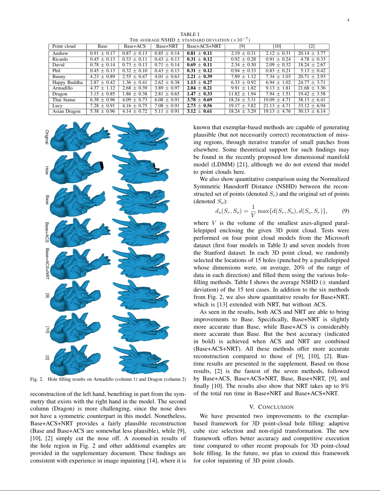
1 Adapti v e Non-Rigid Inpainting of 3D Point Cloud Geometry Chinthaka Dinesh, Student Member , IEEE, Iv an V . Baji ´ c, Senior Member , IEEE, and Gene Cheung, Senior Member , IEEE Abstract —In this letter , we introduce se veral algorithms for geometry inpainting of 3D point clouds with large holes. The algorithms are examplar-based: hole filling is performed itera- tively using templates near the hole boundary to find the best matching regions elsewhere in the cloud, from where existing points are transferred to the hole. W e propose two improv ements over the previous work on exemplar -based hole filling. The first one is adaptive template size selection in each iteration, which simultaneously leads to higher accuracy and lower execution time. The second improvement is a non-rigid transformation to better align the candidate set of points with the template befor e the point transfer , which leads to even higher accuracy . W e demonstrate the algorithms’ ability to fill holes that are difficult or impossible to fill by existing methods. Index T erms —Hole filling, 3D point cloud, 3D geometry in- painting, point cloud alignment, non-rigid transf ormation I . I N T R O D U C T I O N A 3D point cloud consists of a set of points in 3D space, sometimes with attributes such as color . Point clouds are used for representing the geometry of 3D objects and scenes. Recent adv ances in 3D scanning technologies are making 3D point clouds popular in augmented reality , mobile mapping, gaming, 3D telepresence, scanning of historical artifacts, and 3D printing. Howe ver , the scanned 3D point cloud may be missing data in certain regions due to occlusion, low re- flectance of the scanned surface, limited number of scans from different viewing directions, etc. [1]. In certain applications such as remote telepresence, parts of the point cloud may be lost due to unreliable communication links along the way . Hence, filling in the missing regions (holes) is an important problem in 3D point cloud processing. There are a number of methods for detecting holes in point clouds based on v ariations of the point density [2], [3], [4]. In remote telepresence, point cloud data is ordered and packetized for transmission to a remote location. Here, missing packets’ indices can be used to determine the locations in 3D space where the missing data used to be. In this letter , we assume that the hole has been identified using one of these e xisting methods. V arious methods hav e been proposed for hole filling of surfaces represented by meshes [5], [6], [7], [8], but the related problem of hole filling for 3D point clouds has receiv ed less attention. In [9], a triangle mesh is constructed from the input point cloud, then the missing region is interpolated C. Dinesh and I. V . Baji ´ c are with the School of Engineering Science, Simon Fraser Uni versity , Burnaby , BC, Canada, e-mail: hchintha@sfu.ca and ibajic@ensc.sfu.ca. G. Cheung is with National Institute of Informatics, T okyo, Japan, e-mail: cheung@nii.ac.jp. using a moving least squares approach. Howe ver , this method produces unsatisfactory results on lar ge holes, especially if the underlying surface is complex. In [10], a plane tangent to the missing part is determined and the hole boundary is projected onto this plane. Then, its conv ex hull is computed and points are created in such a way that the sampling allo ws to cover a dilated version of the conv ex hull. Next, a k -nearest neighbors graph is constructed from the union of input point cloud and this set of created points. Finally , a graph-based Partial Differential Equation (PDE) solver is used to deform the generated points to fit into the hole. This method gi ves good results for small holes or smooth surfaces, but it faces problems if the hole boundary contains folds or twist. In [2], a hole-filling method based on the tangent plane for each hole boundary point is proposed. T rav ersing the boundary in a clock-wise direction, points on each tangent plane are computed and inserted into the hole. This process is repeated from the hole boundary towards the interior . While this works for small holes, it faces the same problems as [9], [10] on large holes and comple x surfaces. A few methods have been proposed to fill relativ ely large holes in 3D point clouds. In [11], a non-iterativ e framew ork based on T ensor V oting is proposed to fill-in holes by using neighbourhood surface geometry and geometric prior deri ved from registered similar models. In [12], a hole is filled by propagating local 3D surface smoothness from around the hole by harvesting the cues provided by a similar model. Although they can fill large holes reasonably well, both methods need at least one complete model similar to the model with the hole. Recently , we proposed an ex emplar-based framework [13] for hole filling, which exploits non-local self similarity to provide plausible reconstruction ev en for large holes and complex surfaces. This approach is inspired by [14] and its success in image inpainting. The main focus of [13] was on the technical challenges in volved in transplanting the image-based method from [14] into the point-cloud frame work. In this letter , two nov el concepts are proposed to improve our previous framework [13]. The first one is adaptiv e tem- plate size selection to match the local surface characteristics. This leads to both higher accuracy and lower execution time compared to [13]. The second improvement is a non-rigid transformation to better align the set of points that will be transferred into the hole with the surface characteristics near the hole. This improvement further increases the accurac y . A brief revie w of our previous hole-filling method [13] is presented in Section II, followed by the proposed improve- ments in Section III, experimental comparison with [13], [9], 2 Fig. 1. Illustration of the source region Φ , hole Ω and fill front δ Ω . [10], [2] in Section IV, and conclusions in Section V. I I . B R I E F R E V I E W O F [ 1 3 ] The set of av ailable points in the point cloud is called the source r e gion , denoted Φ . The hole is denoted Ω , and its boundary is denoted δ Ω . The boundary ( fill fr ont ) e volves inwards as hole filling progresses. A cube centered at point q , with edges parallel to the x, y , z axes, is denoted ψ q . Fig. 1 illustrates these concepts. The size of each cube in [13] is 10 × 10 × 10 vox els. Here, voxel is a cubic unit of space. T o determine the voxel size for a giv en input cloud, we perform octree partitioning until each cloud point resides in its own vox el, then the smallest voxel size in the octree is taken as the vox el size for that cloud. Octree partitioning is started with a cubic bounding box that encapsulates the whole point cloud. If the partitioning stops after n steps, the volume of the smallest vox el is 2 − 3 n of the volume of the original bounding box. Hole filling consists of three steps – priority calculation, template matching, and point transfer – applied iterativ ely until the hole is filled. Each step is e xplained below . Priority Calculation: The first step is to assign priority to each ψ p for p ∈ δ Ω . The priority is biased to wards those ψ p ’ s that seem to be on the continuation of ridges, valleys, and other surface elements that could more reliably be extended into the hole. For a giv en ψ p , the priority P ( p ) is defined as P ( p ) = D ( p ) C ( p ) , (1) where D ( p ) is the data term, which depends on the structure of the data in ψ p as discussed in [13], and C ( p ) is the number of av ailable points in ψ p ( C ( p ) = | ψ p ∩ Φ | ). T emplate Matching: Once all priorities on the fill front hav e been computed, the highest priority cube ψ b p is selected as b p = arg max p ∈ δ Ω P ( p ) . The av ailable points in ψ b p are called the template . Then, the source region is searched for the cube ψ q ( ψ q ⊂ Φ ) that best matches this template. As dis- cussed in [13], many candidate cubes can be eliminated during the search to speed up the process. T o find the best match for ψ b p among the candidate cubes, ψ q is first translated such that point q coincides with b p . This translated ψ q is denoted ψ q . Then, the best 3D rotation matrix R b is determined to align ψ q with ψ b p , and the rotated cube is denoted ψ R b q . Specifically , the rotation matrix is found as R b = arg min R d  ψ R q , ψ b p  , (2) where R is a 3D rotation matrix and d ( ψ R q , ψ b p ) is the One- sided Hausdorff Distance (OHD) [15] from ψ b p to ψ R q , d  ψ R q , ψ b p  = max a ∈ ψ b p min b ∈ ψ R q k a − b k 2 , (3) where k·k 2 is the Euclidean norm. The Iterative Closest Point (ICP) algorithm [16] is used to find R b in (2) for each candidate cube ψ q , and the correspond- ing OHD after alignment, d ( ψ R b q , ψ b p ) , is recorded. According to [16], the complexity of finding R b is O ( N 1 log N 2 ) , where N 1 and N 2 are the numbers of points in ψ b p and ψ R b q , respectiv ely . Then the rotated cube with the smallest aligned OHD, ψ R b b q , is selected for transfer . Specifically , ψ R b b q = arg min ψ R b q d  ψ R b q , ψ b p  . (4) Point T ransfer: First, the points of ψ R b b q are matched with those of ψ b p . Let x i ∈ ψ b p be a point in ψ b p . Let y i be the closest (by Euclidean distance) point to x i within ψ R b b q , y i = arg min y ∈ ψ R b b q k y − x i k 2 . (5) Then we say that y i has been matched with x i and we add it to the set of matched points of ψ R b b q , denoted M b q . Finally , all the unmatched points, ψ R b b q \ M b q are transferred to ψ b p and the fill front is updated. This completes one iteration of the filling procedure; after this, the fill front δ Ω is updated and the process repeated until the hole is filled. The filling stops at the iteration in which the template covers the entire fill front. I I I . P R O P O S E D M E T H O D S Although [13] outperforms existing methods such as [9], [10], [2], there is still room for improvement. T wo such improv ements are described here: 1) adaptiv e cube size (A CS) for template selection, and 2) non-rigid transformation (NR T) for improved alignment between the template and the best- matched cube. W ith those modifications, the size of the template cube ψ b p will change depending on the surface characteristics, and a non-rigid transformation will be applied to the best-matched candidate cube prior to point transfer . Details are provided in the following sections. A. Adaptive Cube Size The fixed template cube size, as used in [13], may be inappropriate in sev eral cases. For example, when the surface is relativ ely flat near b p , small cube size may lead to finding an inaccurate match elsewhere in the model where the surface is also relativ ely flat. In such a case, the template needs to be increased in order to capture sufficiently discriminative surface structure. There are also other cases where the surface characteristics near b p are so complicated that ev en the best- matched cube of a giv en size is poorly matched to the template, i.e. produces large OHD. T ransferring the points from that cube into the hole would not make sense, and it seems more reasonable to try matching with a smaller template size. T o account for the cases mentioned above, we extend template matching with adaptiv e cube size (ACS) selection. Let ψ n q be a cube of size n × n × n vox els, centered at point q , with edges parallel to the x, y , z axes. The smallest cube size we consider is n = 5 . The initial priority is calculated and the highest priority point b p is found with n = 5 . Following the procedure from Section II, we find the best match ψ n b q ∈ Φ 3 Algorithm 1 Matching with Adaptiv e Cube Size 1: Find b p = arg max p ∈ δ Ω t P ( p ) and set n = 5 2: Find the best-matched cube ψ n b q according to (2)-(4) 3: Let  = d  ψ n R b b q , ψ n b p  and T = 1 . 0001 ·  4: Initialize C = n ψ n q i ∈ Φ : d  ψ n R b q i , ψ n b p  ≤ T o 5: while |C | > 1 do 6: n ← n + 2 7: for All ψ n q i ∈ C do 8: if d  ψ n R b q i , ψ n b p  > T then 9: Remov e ψ n q i from C 10: end if 11: end for 12: end while 13: if |C | == 1 then 14: The cube in C (of size n ) is the best match 15: else 16: Best-matched cube of the pre vious size is the best match 17: end if for ψ n b p . Let the rotated and aligned ψ n b q be denoted ψ n R b b q , and let the OHD between this cube and the template be d  ψ n R b b q , ψ n b p  =  . This  giv es us an idea of what kind of matching error we may hope to find for larger cubes. Based on this, we set a matching threshold T = 1 . 0001 ·  . After setting T , we create a set C = { ψ n q 1 , ψ n q 2 , ..., ψ n q N } of all cubes of size n in Φ , such that d  ψ n R b q i , ψ n b p  ≤ T . This is a set of candidate cubes that match well with the template of size n . Then we increase n and eliminate from C all cubes whose matching error exceeds T with the new size. The process repeats until we are in a position to make a decision about the best-matched cube. Specifically , we keep increasing n until C either ends up with only one cube (which is then the best match) or becomes empty . In the latter case, we go back to the previous (lower) cube size and select the cube with the lowest matching error as the best match. The procedure is summarized in Algorithm 1, where |C | represents the number of elements in C . In our implementation, the cube size n increases in steps of 2 , as indicated in step 6 of the algorithm, but other increment schedules are possible. B. Non-Rigid T ransformation Let ψ n R b b q the best-matched cube found above, after rotation to align it with ψ n b p . As in Section II, let M b q be the set of points in ψ n R b b q that are matched with points in ψ n b p , according to (5). Further improvement in the alignment of ψ n R b b q and ψ n b p can be achieved by Non-Rigid Transformation (NR T). The main challenge in dev eloping a NR T in this case is finding the appropriate transformation for the unmatched points (i.e., those in ψ n R b b q \ M b q ). T o overcome this challenge, we propose the following strategy: the matched points (those in M b q ) will be transformed to minimize their distance to their matches in ψ n b p , while the unmatched points will be transformed in a way that encourages the smoothness of transformation among neighboring points in ψ n R b b q . The NR T we will apply to ψ n R b b q is a collection of affine transformations { T i } , where T i is a 3 × 3 matrix applied to y i ∈ ψ n R b b q . F or the matched points, we define the distortion term D = X y i ∈ M b q k x i − T i y i k 2 2 , (6) where x i ∈ ψ n b p is the point in ψ n b p matched with y i according to (5). In order to take unmatched points into account, we construct an undirected k -nearest neighbor graph ( k = 5 in our case) with points in ψ n R b b q as vertices. Let E be the set of edges in this graph. Then we define the smoothness term S = X ( y i , y j ) ∈ E k T i − T j k F , (7) where k·k F is the Frobenius norm. Finally , the total cost is the combination of the distortion term and the smoothness term, J = D + λS, (8) where λ is the parameter that allows a trade-off between D and S in the cost function. In our experiments, we set λ = 1 . If we define a block matrix T = [ T 1 . . . T N 2 ] T , where N 2 is the number of points in ψ n R b b q , then, follo wing [17], J is a quadratic function of T . Hence, T that minimizes J can be found in closed-form, and the complexity of computing it is O ( N 3 2 ) . F or details, please refer to section 4.2 in [17]. After optimal T i ’ s are found, they are applied to all points in ψ n R b b q . Then the unmatched points of the transformed ψ n R b b q are found and transferred to the hole, as described in Section II. I V . E X P E R I M E N TA L R E S U LT S W e test the proposed hole filling framew ork on 3D point clouds from two datasets: the Microsoft V oxelized Upper Bodies [18] and the Stanford 3D Scanning Repository [19]. There are mesh models in the Stanford dataset and here we stripped away the mesh connectivity and used vertices as a point cloud. Howe ver , the models in the Microsoft data set are real point clouds captured by four depth cameras. Both qualitativ e and quantitative results are presented and compared to those of [13], [9], [10], [2]. For this purpose, we implemented [9], [10], [2] follo wing the papers. Holes were generated in 3D point clouds by removing all points in a relatively large parallelepiped whose sides were aligned with x , y , and z axes. Hole filling results for such generated holes are sho wn in Fig. 2 for two point cloud models from the Stanford dataset. In this figure, the point clouds are rendered using MeshLab software tool [20]. The first row shows the original point cloud/surface, second row shows the hole, while rows three to eight show the results of hole filling by the method in [13] (referred to as Base), [13] extended with A CS (Base+A CS), [13] extended with both ACS and NR T (Base+A CS+NR T) and those of [9], [10], [2], respectiv ely . As seen in the figure, both Base+ACS and Base+A CS+NR T improv e the reconstruction of the underlying surface compared to Base. All these three methods provide better reconstruction than [9], [10], [2]. The results in the first column (Armadillo) show that Base+A CS and Base+ A CS+NR T provide f airly good 4 T ABLE I T H E A V E R A G E N S H D ± S T A N D A R D D E V I A T I O N ( × 10 − 7 ) Point cloud Base Base+A CS Base+NR T Base+A CS+NR T [9] [10] [2] Andre w 0.91 ± 0.17 0.87 ± 0.13 0.85 ± 0.14 0.81 ± 0.11 2.19 ± 0.31 2.12 ± 0.31 20.14 ± 3.77 Ricardo 0.45 ± 0.13 0.33 ± 0.11 0.43 ± 0.13 0.31 ± 0.12 0.92 ± 0.28 0.91 ± 0.24 4.78 ± 0.33 Da vid 0.78 ± 0.14 0.73 ± 0.13 0.71 ± 0.14 0.69 ± 0.11 2.34 ± 0.30 2.09 ± 0.32 18.24 ± 2.67 Phil 0.45 ± 0.13 0.32 ± 0.10 0.43 ± 0.13 0.31 ± 0.12 0.94 ± 0.33 0.83 ± 0.21 5.13 ± 0.42 Bunn y 4.23 ± 0.89 2.55 ± 0.47 4.01 ± 0.63 2.21 ± 0.39 7.89 ± 1.12 7.34 ± 1.03 20.71 ± 2.93 Happ y Buddha 2.87 ± 0.42 1.36 ± 0.41 2.62 ± 0.38 1.13 ± 0.27 6.33 ± 0.92 6.94 ± 1.02 24.77 ± 3.71 Armadillo 4.37 ± 1.12 2.68 ± 0.39 3.89 ± 0.97 2.04 ± 0.21 9.91 ± 1.82 9.13 ± 1.81 21.68 ± 3.36 Dragon 3.15 ± 0.85 1.86 ± 0.38 2.81 ± 0.65 1.47 ± 0.33 11.82 ± 1.94 7.94 ± 1.51 19.42 ± 3.58 Thai Statue 6.38 ± 0.96 4.09 ± 0.73 6.08 ± 0.91 3.78 ± 0.69 18.24 ± 3.31 19.09 ± 4.71 38.13 ± 6.41 Luc y 7.28 ± 0.91 4.16 ± 0.75 7.08 ± 0.91 2.73 ± 0.56 19.17 ± 3.82 21.13 ± 4.71 33.12 ± 6.94 Asian Dragon 5.38 ± 0.96 4.14 ± 0.72 5.11 ± 0.91 3.12 ± 0.61 18.24 ± 3.29 19.13 ± 4.76 30.13 ± 6.14 Fig. 2. Hole filling results on Armadillo (column 1) and Dragon (column 2) reconstruction of the left hand, benefiting in part from the sym- metry that e xists with the right hand in the model. The second column (Dragon) is more challenging, since the nose does not ha v e a symmetric counterpart in this model. Nonetheless, Base+A CS+NR T pro vides a f airly plausible reconstruction (Base and Base+A CS are some what less plausible), while [9], [10], [2] simply cut the nose of f. A zoomed-in results of the hole re gion in Fig. 2 and other additional e xamples are pro vided in the supplementary document. These findings are consistent with e xperience in image inpainting [14], where it is kno wn that e x emplar -based methods are capable of generating plausible (b ut not necessarily correct) reconstruction of miss- ing re gions, through iterati v e transfer of small patches from else where. Some theoretical support for such findings may be found in the recently proposed lo w dimensional manifold model (LDMM) [21], although we do not e xtend that model to point clouds here. W e also sho w quantitati v e comparison using the Normalized Symmetric Hausdorf f Distance (NSHD) between the recon- structed set of points (denoted S r ) and the original set of points (denoted S o ): d s ( S r , S o ) = 1 V max { d ( S r , S o ) , d ( S o , S r ) } , (9) where V is the v olume of the smallest ax es-aligned paral- lelepiped enclosing the gi v en 3D point cloud. T ests were performed on four point cloud models from the Microsoft dataset (first four models in T able I) and se v en models from the Stanford dataset. In each 3D point cloud, we randomly selected the locations of 15 holes (punched by a parallelepiped whose dimensions were, on a v erage, 20% of the range of data in each direction) and filled them using the v arious hole- filling methods. T able I s ho ws the a v erage NSHD ( ± standard de viation) of the 15 test cases. In addition to the six methods from Fig. 2, we also sho w quantitati v e results for Base+NR T , which is [13] e xtended with NR T , b ut without A CS. As seen in the results, both A CS and NR T are able to bring impro v ements to Base. Specifically , Base+NR T is slightly more accurate than Base, while Base+A CS is considerably more accurate than Base. But the best accurac y (indicated in bold) is achie v ed when A CS and NR T are combined (Base+A CS+NR T). All these methods of fer more accurate reconstruction compared t o those of [9], [10], [2]. Run- time results are presented in the supplement. Based on those results, [2] is the f astest of the se v en methods, follo wed by Base+A CS, Base+A CS+NR T , Base, Base+NR T , [9], and finally [10]. The results also s h o w that NR T tak es up to 8% of the total run time in Base+NR T and Base+A CS+NR T . V . C O N C L U S I O N W e ha v e presented tw o impro v ements to the e x emplar - based frame w ork for 3D point-cloud hole filling: adapti v e cube size selection and non-rigi d transformation. The ne w frame w ork of fers better accurac y and competiti v e e x ecution time compared to other recent proposals for 3D point-cloud hole filling. In the future, we plan to e xtend this frame w ork for color inpainting of 3D point clouds. 5 R E F E R E N C E S [1] S. Setty , S. A. Ganihar, and U. Mudenagudi, “Framew ork for 3D object hole filling, ” in Proc. IEEE NCVPRIPG , Dec. 2015, pp. 1–4. [2] V . S. Nguyen, H. T . Manh, and T . N. T ien, “Filling holes on the surf ace of 3D point clouds based on tangent plane of hole boundary points, ” in Pr oc. ACM SoICT , 2016, pp. 331–338. [3] G. H. Bendels, R. Schnabel, and R. Klein, “Detecting holes in point set surfaces, ” in Pr oc. WSCG’06 , Jan.-Feb. 2006. [4] V . S. Nguyen, T . H. Trinh, and M. H. T ran, “Hole boundary detection of a surface of 3D point clouds, ” in Proc. IEEE A COMP’15 , Nov . 2015, pp. 124–129. [5] T . Ju, “Robust repair of polygonal models, ” ACM T rans. Graph. , v ol. 23, no. 3, pp. 888–895, 2004. [6] J. Podolak and S. Rusinkie wicz, “ Atomic volumes for mesh completion, ” in Symposium on Geometry Pr ocessing , 2005, pp. 33–41. [7] W . Zhao, S. Gao, and H. Lin, “ A robust hole-filling algorithm for triangular mesh, ” V isual Comput. , vol. 23, no. 12, pp. 987–997, 2007. [8] J. X. Wu, M. Y . W ang, and B. Han, “ An automatic hole-filling algorithm for polygon meshes, ” Computer-Aided Design and Applications , v ol. 5, no. 6, pp. 889–899, 2008. [9] J. W ang and M. M. Oliv eira, “Filling holes on locally smooth surfaces reconstructed from point clouds, ” Image and V ision Computing , vol. 25, no. 1, pp. 103–113, Jan. 2007. [10] F . Lozes, A. Elmoataz, and O. Lezoray , “PDE-based graph signal pro- cessing for 3-D color point clouds: Opportunities for cultural heritage, ” IEEE Signal Process. Mag. , vol. 32, no. 4, pp. 103–111, 2015. [11] P . Sahay and A. N. Rajagopalan, “Harnessing self-similarity for recon- struction of large missing regions in 3d models, ” in IEEE International Confer ence on P attern Recognition (ICPR) , 2012, pp. 101–104. [12] ——, “Geometric inpainting of 3d structures, ” in IEEE Confer ence on Computer V ision and P attern Recognition W orkshops , 2015, pp. 1–7. [13] C. Dinesh, I. V . Bajic, and G. Cheung, “Exemplar -based framew ork for 3d point cloud hole filling, ” in IEEE VCIP , 2017, pp. 1–4. [14] A. Criminisi, P . Perez, and K. T oyama, “Region filling and object remov al by e xemplar -based image inpainting, ” IEEE T rans. Image Pr ocess. , vol. 13, no. 9, pp. 1200–1212, Sept. 2004. [15] P . Cignoni, C. Rocchini, and R. Scopigno, “Metro: Measuring error on simplified surfaces, ” Computer Gr aphics F orum , v ol. 17, no. 2, pp. 167– 174, 1998. [16] S. Rusinkiewicz and M. Lev oy , “Efficient variants of the ICP algorithm, ” in Int. Conf. 3-D Digital Imaging and Modeling , 2001, pp. 145–152. [17] B. Amberg, S. Romdhani, and T . V etter , “Optimal step nonrigid ICP algorithms for surface registration, ” in IEEE Confer ence on Computer V ision and P attern Recognition , 2007, pp. 1–8. [18] C. Loop, Q. Cai, S. O. Escolano, and P . A. Chou, “Microsoft voxelized upper bodies - a v oxelized point cloud dataset, ” in ISO/IEC JTC1/SC29 Joint WG11/WG1 (MPEG/JPEG), m38673/M72012 , 2016. [19] M. Levo y , J. Gerth, B. Curless, and K. Pull, “The Stanford 3D scanning repository , ” [Online] https://graphics.stanford.edu/data/3Dscanrep/. [20] P . Cignoni, M. Callieri, M. Corsini, M. Dellepiane, F . Ganovelli, and G. Ranzuglia, “Meshlab: an open-source mesh processing tool. ” in Eur ographics Italian Chapter Conference , vol. 2008, 2008, pp. 129– 136. [21] S. Osher, Z. Shi, and W . Zhu, “Low dimensional manifold model for image processing, ” SIAM Journal on Imaging Sciences , vol. 10, no. 4, pp. 1669–1690, 2017.