Efficient Bayesian Multivariate Surface Regression

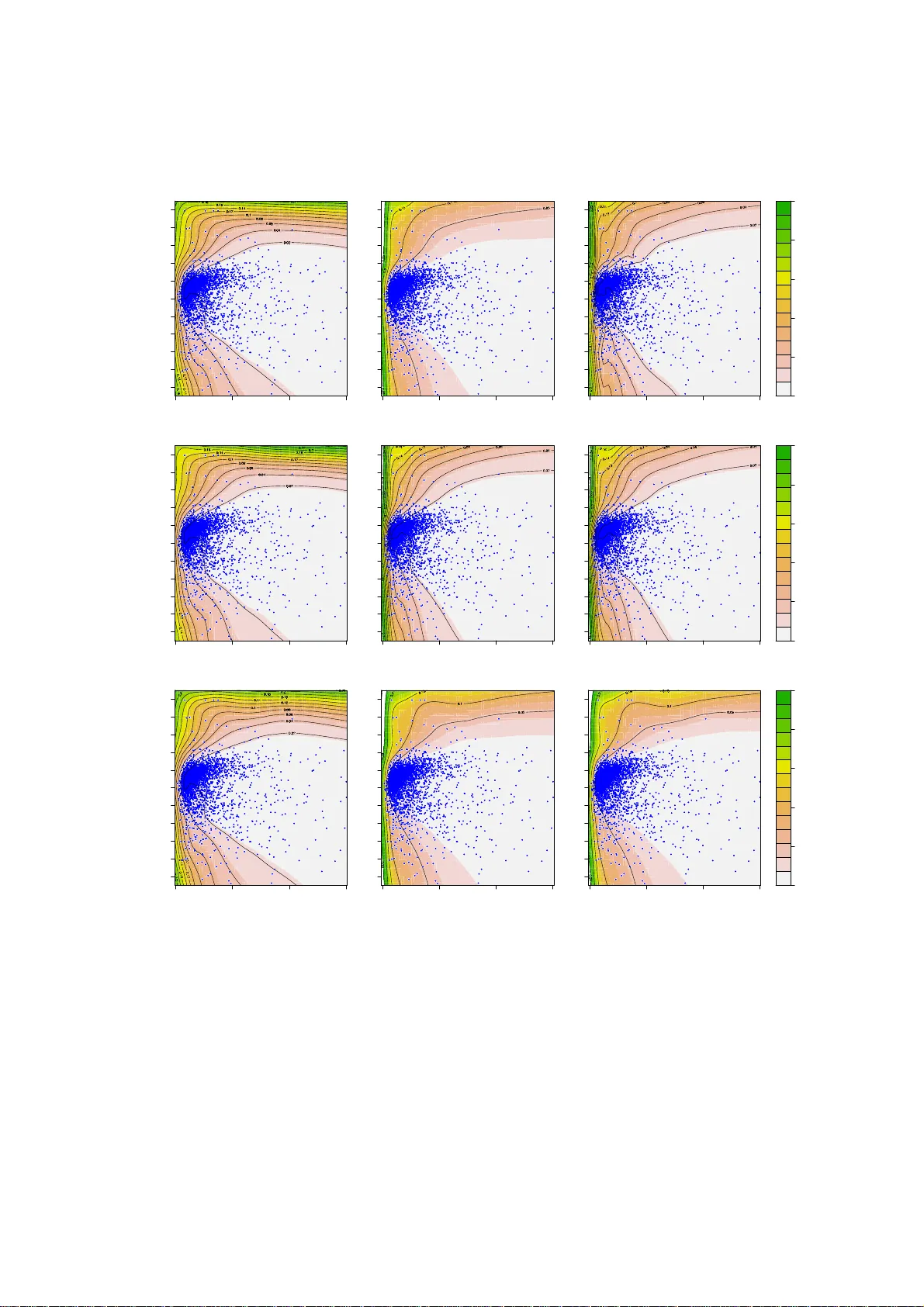
EFFICIENT BA YESIAN MUL TIV ARIA TE S URF ACE REGRESSION FENG LI AND MA TTIAS VILLANI Abstract. Metho ds for choosing a ﬁxed set of knot lo cations in additive spline mo dels are fairly well established in the statistical liter a ture. While most of these metho ds a re in principle directly extendable to non-a dditiv e surface models, they are less likely to be successful in that setting becaus e of the curse of dimensionality , espe c ia lly when there are more than a couple of cov ariates. W e prop ose a regres sion model for a multiv ariate Gaussian resp onse that combines b oth additiv e splines and interactive splines, and a hig hly eﬃcient MCMC algorithm that updates all the knot loca tio ns joint ly . W e use shrink age priors to av oid ov erﬁtting with diﬀ erent estimated shrink age factors for the additiv e and surface par t of the mo del, a nd also diﬀeren t shr ink a ge parameters for the diﬀerent r esponse v aria bles. This makes it p ossible for the model to a dapt to v arying degrees of no nlinea rit y in diﬀerent parts of the data in a pars imonious wa y . Sim ulated da ta and an a pplication to ﬁrm leverage data show that the appr oac h is computationally eﬃcient, a nd that a llo wing for freely estimated knot loca tions can o ﬀer a substanti al improvemen t in out-of-sample predictiv e p erformance. Keyw ords : Ba y esian inference, Markov c hain Mont e Carlo , Surface regr e ssion, Splines, F ree knots. 1. Introduction Flexible mo dels of the regression function E( y | x ) has b een an activ e researc h ﬁeld for decades, see e.g. Rupp ert et al. (2003) for a recen t t extb o ok in tro duc tion and f urther ref- erences. In tens iv e researc h w a s ini tially dev oted to k ernel regressi on metho ds (Nadara y a 1964, W atson 1964 , Gasser & Müller 1979), and later follow ed b y a large literature on spline regression mo deling. A spline is a linear regression o n a set of nonlinear basis functions of the original regress ors. E ac h basis function is deﬁne d from a knot in regressor space and the knots determine the p oints of ﬂexibilit y of the ﬁtted regression function. Th is giv es rise to a lo cally adaptable mo del with con tin uit y at the knots. Li (corresp onding author): Department of Statistics, Sto c kholm Univ ersit y , SE-106 91 Stockholm, Sweden. E-mail: feng. li@stat.s u .se . Villani: Division of Statistics, Department of Computer and Information Science, Linköping Univ ersit y , SE-581 83 Linköping, Sweden. E-mail: matti as.villan i @liu.se . 1 EFFICIENT BA YESIA N MUL TIV ARIA TE SURF ACE REGRES SION 2 The most widely used mo dels assume additivit y in the regressors, i.e. E( y | x 1 , ..., x q ) = P q j =1 f j ( x j ) , where f j ( x j ) is a spline function for the j th regressor (Hastie & Tibshi rani 1990). Assuming additivit y is cle arly a v ery con v enien t simpliﬁcation, but it is also some- what unnatural to mak e suc h a strong assump tion in an otherwise v ery ﬂexible mo del. This has motiv a ted researc h o n surface mo dels with in teractions betw een regressors. One line of researc h extend s the additiv e mo dels b y including higher-order in teractions of the spline basis functions, see e.g. the struc tured ANO V A approach or the tensor pro duct basis in Hastie et al. (2009). The m ultiv aria te adaptiv e regression splines (MARS) in tro duce d in F riedman (1991) is a vers ion of the tensor pro duct spline with in terac tions sequen tially en- tering the mo del using a greedy algorithm. Regress ion trees (Breiman et al. 1984) is another p opular class of mo dels, with the BAR T mo del in Chipman et a l. (2010) as its most pro mi- nen t Ba y esian mem b er. Our pap er follo ws a recen t strand of literature that mo dels surfaces using radial basis functions splines, see e.g. Buhmann (2003). A radial basis f unction is deﬁned in R q and has a v a lue that dep ends only on the distance from a co v aria te v ector ( x ) to its q -dimensional knot ( ξ ), e.g. the cubic radial basis k x − ξ k 3 , where x = ( x 1 , ..., x q ) ′ , ξ = ( ξ 1 , ..., ξ q ) ′ and k·k is the Euclidean norm. The mo del is again linear in the basis expanded space. The basic c hallenge in spline regression is the c hoice o f knot lo cations. This problem is clearly muc h harder for a general surface tha n it is fo r additiv e models since an y manage- able set of q -dimensional knots are nec essarily sparse in R q when q is mo derate or large, a manifestation of the curse of dimensionalit y . The state-of -the-art inferen tial pro cedure s place the knots a t the cen troids fr o m a clustering of t he regressor observ ations. Th e selected knot lo cations are k ept ﬁxed throughout the analysis. T o prev ent ov erﬁtting, Bay esian v ariable selection metho ds are used to automatically remo v e or down w eigh t the inﬂuence of the knots using Mark o v chain Mon te Carlo ( MCMC) metho ds (Smith & K ohn 1996). The reve rsible jump MCMC (RJMCMC) in for example Denis on et al. (2002) treats the n um ber of knots as unkno w n sub ject to an upper b ound, but the lo cation o f the knots are still ﬁxed throughout the analysis. Using a ﬁxed set of knot lo cations is impractical when estimating a surface with more than a few regressors. An algorithm that can mo v e the knots rapidly ov er the regressor space is ex- p ected to b e a clear impro v emen t. All previous attempts hav e fo cused on eﬃcien t selection of ﬁxed knots, a nd ha v e paid little attention to mo ving the knots. The o therw ise v ery elab orate RJMCMC approac hes in Dimatteo et al. (20 0 1 ), Denison et al. (1998), Gulam Razul et al. EFFICIENT BA YESIA N MUL TIV ARIA TE SURF ACE REGRES SION 3 (2003) and Holmes & Mallic k (2003) all include a v ery simple MCMC up date where a single knot is re-lo cated using a Metrop olis random w alk step with a prop osal v ariance that is the same for all knots. There are typic ally strong dep enden cies b et w e en the knots, and lo cal one- knot-at-a-time mov es will lead to slo w conv ergence of the algorithm and inability to escape from local mo des, see Section 5.4 for some evidence. This is esp ecially true in the surface case with more than a couple of regressors. The main con tribution in this pap er is a highly eﬃcien t MCMC algorithm for the Gaussian m ultiv ariate surface regression where the lo cations of all knots are updated join tly . Rapid mixing of the knot lo catio ns is obtained from the follo wing t wo features of our algorithm. First, the knots are sim ulated from a marginal p osterior where the high- dimensional regres - sion co eﬃcien ts hav e been integrated out a nalytic ally . Second, the knots’ prop osal distri- bution is tailored to the posterior distribution using the p osterior gradien t, whic h w e deriv e in compact analytical for m a nd ev a luat e eﬃcien t ly b y a careful use of sparsit y . W e use a shrink a ge prior on the regression co eﬃcie n ts to prev en t ov erﬁtting, where the shrink age h y- p erparameters a r e treated as unkno wns and are estimated in a separate up dating step. Also this step is tailored to the p osterior using the gradien t in analytical form. Ev en a highly eﬃ cien t MCMC algo rithm is lik ely to ha v e problems exploring the jo in t p osterior of man y surface knots in a high- dime nsional co v ar ia t e space. T o deal with this, our mo del is decomp osed in to three parts: i) the original co v a ria tes en t ering in linear f orm, ii) additiv e spline basis functions and iii) radial basis functions for capturing the remaining part of the surface and interac tions. The idea is to let the additiv e part o f the mo del capture the bulk of the nonlinearities so that the radial basis f unc tions can fo cus exclusiv ely on mo deling the inte ractions. This w ay w e can k e ep the n um b er of knots in the in teraction part of the mo del to a minim um, whic h is b eneﬁcial for MCMC con v ergence. W e use separate shrink ag e priors for the three parts of the mo del. Moreo v er, w e also allow for separate shrink age parameters in eac h resp onse equation. This giv es us an extremely ﬂexible yet p oten tially parsimonious mo del whe re w e can shrink out e.g. the surface part of the mo del in a subset of the resp o ns e equations. Our MCMC sc heme is designed fo r a ﬁxed n um b er of knots, and w e select the num b er of knots b y Ba y e sian cross -v alidation o f the log predictiv e score using para lle l computing, see Section 3.3. This has the disadv an tage o f not accoun ting fo r the uncertain ty regarding the n um b er of knots as is done in RJMCMC sc hemes , but the b ene ﬁts are substan tially more robustness to v ariations in the prior and impro v ed MCMC eﬃcien cy . EFFICIENT BA YESIA N MUL TIV ARIA TE SURF ACE REGRES SION 4 W e illustrate our algorithm on sim ulated and real data, and compare the predictiv e p erfor- mance of the mo dels using Bay esian cross-v alidation tec hniq ues. W e ﬁnd that the free knots mo del constan tly outp erforms the mo del with ﬁxed knots. A dditionally , we ﬁnd it is easie r to obtain b etter ﬁtting res ult b y com bining additiv e knots and surface knots in the mo del. 2. Ba yesian mul t iv aria te surf ace regr ession 2.1. The mo del. Our prop osed mo del is a Gaussian m ultiv ariat e regression with three sets of co v aria tes : Y = X o B o + X a ( ξ a ) B a + X s ( ξ s ) B s + E , (1) where Y ( n × p ) con ta ins n observ ations on p res p onse v ariables, and the ro ws of E are error v ectors assumed to b e iid N p ( 0 , Σ ) . The matrix X o ( n × q o ) con tains the original regressors (ﬁrst column is a v ector of ones for the in tercept) and B o holds the corresponding regression co eﬃcien ts. The q a columns of the matrix X a ( ξ a ) a re additiv e splines functions of the co v ariates in X o . Our notation mak es it clear that X a dep end s on the knots ξ a . Note that the knots in the additiv e part of the mo del are scalars, and that our mo del allo ws for unequal n um b er of knots in the diﬀeren t co v aria tes. Finally , X s ( ξ s ) con tains the surface, or in teraction, part of the mo del. The knots in ξ s are q o -dimensional v ectors. Note ho w this decompo sition mak es it p ossible for the additiv e part o f the mo del to capture the main part of the nonlinearities so that the n umber of knots in X s is k ept to a minim um. W e will refer to the three diﬀeren t parts of the mo del as the line ar c om p onent , the additive c omp onent and the surfac e c omp onent , respectiv ely . W e will refer to ξ a and ξ s as the additiv e and surface knots, respectiv ely . Lik ewise, B a and B s are the additiv e and surface co eﬃcien ts. There are a large num b er of diﬀeren t spline bases that one can use for the additiv e part of the mo del. The men u of ch oices fo r the surface basis is mor e limited, see Denis on et al. (2002) for a surv ey o f the most commonly used bases. W e will use thin-plate splines for illustration, but our approach can b e used with any basis with trivial c hanges, see Section 3 and App endix A for computational details. The thin-plate spline basis in the surface case is of the form x sj ( ξ sj ) = k x o − ξ sj k 2 ln k x o − ξ sj k , j = 1 , ..., q s , (2) where x o is one of the original data p oin ts and ξ sj is the j th q o -dimensional surface knot. The univ ar ia t e thin-plate basis used in the additiv e part is a sp ecial case of the m ultiv ariate thin-plate in (2) where b oth the data p oin t and the knot are one-dimensional. EFFICIENT BA YESIA N MUL TIV ARIA TE SURF ACE REGRES SION 5 F or notational con v enience, w e sometimes write mo del (1) in compact form Y = X B + E , where X = [ X o , X a , X s ] is the n × q design mat rix ( q = q o + q a + q s ) and B = [ B ′ o , B ′ a , B ′ s ] ′ . Deﬁne also b i = v ec B i as the v ectorization of the co eﬃcien ts matr ix B i , and b = [ b ′ o , b ′ a , b ′ s ] ′ . F or a giv en set of ﬁxed knot lo cations, the mo del in (1) is linear in the regression co eﬃci en ts B . As explaine d in the Introduction, the great challe nge wi th spline mo dels is the c hoice of knot locations. This is especially true in t he surface case where the curse of dime nsionalit y mak es it really hard to distribute the m ulti-dimensional knots in R q o in an eﬀectiv e w a y . T o get a fair cov erage of knots in the co v ariate space , a recommended approac h is to place the knots at the clus ter cen ters from some clus tering algorithm, e.g. k -means clustering or using a mixture of m ultiv ariat e normals, see Smith & K ohn (1996) and Denison et al. (1998). This t ypically leads to man y redundan t knots (since the resp onse v ariables are not used to aid the clustering) whic h is a source o f o v erﬁtting. One solution is to remov e (do wn w eigh t) the knots b y Bay esian v ariable selection (Smith & Kohn 1 996), p ossibly in a RJMCMC approac h, see e.g. Dimatteo et al. (2001) and Denis on et al. (2002). Nev ertheless, using a set of pre- determined knots is unlik ely to work w ell in the surface case with more than a handful of regressors. W e will treat the knot lo cations in ξ a and ξ s as unkno wn parameters to b e estimated. This is in principle straightforw ard from a Ba ye sian p o in t of view, but great care is needed in the actual implemen tation of the p osterior computations. W e prop ose an eﬃcien t MCMC sc he me for sampling from the join t posterior of the all kn ot lo cations and the regression co eﬃcie n ts, see Sec tion 3 f or details. The mo del is clearly highly (o v er)parametrized and in need of some regularization of the parameters. The tw o main regularization tec hniques in Ba y esian analysis are shrink ag e priors a nd v a ria ble (knot) selection priors. V ariable selection can in princ iple be incorp orated in the a nalys is, but w ould b e computationally demanding since the num b er of gradien t ev aluations needed in our MCMC algorithm w ould increase dramatically . This is imp ortan t since ev aluating the gradien t with resp ect to the knots is time-consuming as the knot lo cations en ter the likeli ho o d in a v ery complicated nonlinear w a y ; see Section 3.2 for details. Moreo v er, part o f the at t ra ction of v ariable selection is that they also pro vide inte rpretable measures of v ariable imp ortance; this is m uc h less in teresting here since the co v ariates correspond to knot lo cations, whic h are not interes ting in themselv es . W e ha v e therefore c hosen to ac hieving parsimon y with shrink age priors that pull the regression EFFICIENT BA YESIA N MUL TIV ARIA TE SURF ACE REGRES SION 6 co eﬃcie n ts tow ards zero (or an y other reference p oin t if so desired), see Section 2.2 for details. W e allow fo r separate shrink age parameters for the linear, additiv e a nd surface parts of the mo del, and separate shrink age parameters for the p responses within eac h of the three mo del parts. The shrink age parameters are treated as unkno wns and estimated, so that, for example, the surface part can b e shrunk to w ards ze ro if this agrees with the data. Allo wing the knots to mo v e freely in co v ariate space in tro duces a knot switc hing problem simi lar t o the well-kno wn lab el switc hing problem in mixture mo dels. The lik eliho o d is in v ariant to a switc h o f tw o knot lo cations and their regression co eﬃc ien t s. This lac k of iden tiﬁcation is not imp ortant if our aim is to mo del the regression surface E( y | x ) , without regard to the p osterior of the individual knot lo cations (Gewe k e 2007). Also, the MCMC dra ws of the knot lo cations can also b e used t o construct heat maps in co v ariate space to represen t the densit y of knots in a certain regions, see Sec tion 5. Such heat maps a r e clearly also immune to the knot switc hing problem. 2.2. The prior. W e no w in troduce an easily sp eciﬁed shrink age prior for t he three sets of regression co eﬃci en ts B o , B a and B s and the cov ariance matrix Σ , conditional on the knots. The prior for b and Σ are set as v ec B i | Σ , λ i ∼ N  µ i , Λ 1 / 2 i ΣΛ 1 / 2 i ⊗ P − 1 i  , i ∈ { o, a, s } , Σ ∼ IW ( n 0 S 0 , n 0 ) , with prior independence b et w ee n the B i . The prior mean of ve c B i is µ i , whic h w e set to zero in our shrink age prior. Λ i = diag ( λ i ) = diag ( λ i, 1 , ..., λ i,p ) , P i is a p ositiv e deﬁnite symmetric matrix. IW ( · ) denotes the inv erse Wishart distribution, with lo cation matrix S 0 and degrees of freedom n 0 . P i is typ ically either the iden tit y matrix or P i = X ′ i X i . The la tt er choic e has b een termed a g -prior b y Zellner (1986) and has the adv an tage of automatically adjusting for the diﬀere n t scales of the co v a riates. Setting λ i = n mak es the information con ten t of the prior equiv alen t to a single data point and is usually called the unit information prior. The c hoice of P i = I q i can prev en t the design matrix from falling in to singularit y problem when some o f the basis functions are highly correlated, whic h can easily happ en with many spline knots. See also the discussion in Denison et al. (2002). Our default c hoice is therefore P o = X ′ o X o , P a = I q a and P s = I q s . Other shrink age priors on the regression co eﬃcien ts can b e used in our approach, for example the Laplace distribution leading to the p opular Lasso (Tib shirani 19 96), but they will t ypic ally not a llo w us to in tegrate out the regress ion EFFICIENT BA YESIA N MUL TIV ARIA TE SURF ACE REGRES SION 7 co eﬃce n ts analytically , see Section 3.1. The optimal c hoice of shrink age prior dep ends on the unkno w n data generating mo del (a normal prior is b ette r when a ll coeﬃcien ts hav e r o ughly the same magnitude; La sso is b etter whe n many co eﬃcien ts a r e close to zero, but some are really large etc). W e also estimate the shrink age parameters, λ o , λ a and λ s via a Ba y esian approach. Note that our prior constructions for B allow for se parate shrink age of the linear, additive and surface comp onen ts. This gives us automat ic regularization/shrink age of the regression coef- ﬁcien ts and helps to av oid problems with ov erﬁtting. Our MCMC sche me in Section 3 allows for a user-sp eciﬁed prior on λ ij , for i ∈ { o, a, s } and j = 1 , 2 , ..., p of ess en tially an y func- tional form. Ho w ev er the default prior of λ ij in this pap er f ollo ws a log normal distribution with mean o f n/ 2 and standard dev iation of n/ 2 in order to ensure that b oth tight and ﬂat shrink a ges are a t t a inable within one standard deviation in the prior . F or computational con- v enie nce, w e us e a log link for λ ij and mak e inference on log ( λ ij ) . As a result the preceding prior on λ ij yields a normal prior for log( λ ij ) with mean [log( n ) − 3 / 2 · log (2)] and v ariance log(2) . W e use the same n um b er of additiv e knots for each co v ariate in the sim ulations and the application in Section 4 and 5, but it should b e clear tha t our approach also p ermits unequal n um b er o f knots in the diﬀeren t co v ariates. There is no particular requiremen ts for the prior on the knots, but a v ague prior shoul d p ermit t he knots to mov e freely in co v ariate space. Our default prior assume s indep enden t knot lo cations follo wing a normal distribution. The mean of the knots comes from the cen ters of a k -means clustering of the cov ariates. In the additiv e case, the prior v a riance of all the knots in the k th cov aria te is c 2 ( a ′ a ) − 1 , where a is the k th column of X o . Similarly , the prior co v ariance matrix of a surface knot is c 2 ( X ′ o X o ) − 1 . W e use c 2 = n as the default setting. The h yperparameter S 0 in the IW prior for Σ is set equal to the estimated error co v ariance matrix from the ﬁtted linear mo del ˆ Y = X o ˆ B o . A small degrees of freedom ( n 0 ) giv es diﬀuse prior on Σ and n 0 = 10 is set as the default. F or notational conv enience and further computational implemen tation, w e write the prior for the regression co eﬃcien ts in condensed form as b | Σ , λ ∼ N ( µ ∗ , Σ b ) where λ = ( λ ′ o , λ ′ a , λ ′ s ) ′ , µ ∗ = ( µ ′ o , µ ′ a , µ ′ s ) ′ , Σ b = ( Λ 1 / 2 Σ K Λ 1 / 2 ) > P − 1 , Λ = diag( λ ) , Σ K is a three-blo c k diagonal matrix with Σ on eac h blo c k, P = diag( P o , P a , P s ) is a blo c k diagonal matrix and A > C denotes the Khatri- Rao pro duct (K hatri & R a o 1968) whic h is K ronec k er pro duct of the correspo ndin g blo c ks of matrices A and C . It will also be conv enien t to deﬁne β = vec B . EFFICIENT BA YESIA N MUL TIV ARIA TE SURF ACE REGRES SION 8 Note that b and β con tain the same elemen ts with tw o diﬀeren t stac ki ng orders. As a result, β | Σ , λ ∼ N ( µ , Σ β ) where µ and Σ β essen tially ha v e the same en tries as µ ∗ and Σ b ha v e, respectiv ely (Section A.3). 3. The posterior inference 3.1. The p osterior. T he p osterior distribution can be decomp osed as p ( B , Σ , ξ , λ | Y , X ) = p ( B | ξ , λ , Σ , Y , X ) p ( ξ , λ , Σ | Y , X ) , where v ec B | ξ , λ , Σ , Y , X ∼ N( ˜ β , Σ ˜ β ) , Σ ˜ β = [ Σ − 1 ⊗ X ′ X + Σ − 1 β ] − 1 , ˜ β = v ec ˜ B = Σ ˜ β [v ec( X ′ Y Σ − 1 ) + Σ − 1 β µ ] (Zellner 1971), and p ( ξ , λ , Σ | Y , X ) = c × p ( ξ , λ ) × | Σ β | − 1 / 2 | Σ | − ( n + n 0 + p +1) / 2 | Σ ˜ β | − 1 / 2 × exp  − 1 2  tr Σ − 1  n 0 S 0 + n ˜ S  +  ˜ β − µ  ′ Σ − 1 β  ˜ β − µ   (3) where ˜ S = ( Y − X ˜ B ) ′ ( Y − X ˜ B ) / n , c = 2 − ( n 0 + n + q ) p/ 2 π − p ( n + q ) / 2 Γ − 1 p ( n 0 / 2) | n 0 S 0 | n 0 / 2 , Γ p ( a ) = π p ( p − 1) / 4 Q p j =1 Γ [ a + (1 − j ) / 2] is the m ultiv ariate gamma function. It is importa n t to note that it is in g eneral not p ossible to integrate out Σ analytically in our mo del. This is a conseque nce of using diﬀeren t shrink age factors for the diﬀeren t resp onses and on the original, additiv e and surface parts of the mo del (the prior co v ariance matrix of B do es not ha ve a Kronec k er structure). Only in the sp ecial case with a univ ariate resp onse ( p = 1 ) can w e in tegrate out Σ analytically , since Σ is then a scalar. T o obta in a uniform treatment of the mo dels and their gradien ts, we hav e c hosen to not inte grate out Σ ev en for the case p = 1 . The next subsection prop oses an MCMC algorithm for sampling from the join t p osterior distribution of all parameters. 3.2. The MCMC algorithm. Our approa ch is to sample from p ( ξ , λ , Σ | Y , X ) using a three-blo c k Gibbs sampling algorithm with Metrop olis-Hastings (MH) up dating steps. Dra ws from p ( B | ξ , λ , Σ , Y , X ) can subsequen tly b e obtained b y direct sim ulation. The up dating steps of the Gibbs sampling algorithm are: (1) Simul ate Σ from p ( Σ | ξ , λ , Y , X ) . (2) Simul ate ξ from p ( ξ | λ , Σ , Y , X ) . (3) Simul ate λ from p ( λ | ξ , Σ , Y , X ) . EFFICIENT BA YESIA N MUL TIV ARIA TE SURF ACE REGRES SION 9 In the special case when p = 1 Σ | ξ , λ , Y , X ∼ IW  n 0 S 0 + n ˜ S + X i ∈{ o,a,s } Λ − 1 / 2 i ( ˜ B i − M i ) ′ P i ( ˜ B i − M i ) Λ − 1 / 2 i , n 0 + n  (4) where M i and ˜ B i are the prior and p osterior mean o f B i , resp ectiv ely . A ctually , when p = 1 , Σ is a scalar and the IW densit y reduces to a scaled χ 2 distribution. When p > 1 , p ( Σ | ξ , λ , Y , X ) is no longer IW , but the distribution in (4) is an exc ellen t approx imation and can b e used as a ve ry eﬃcien t MH prop osal densit y . The conditional p osterior distributions for ξ and λ in Steps (2) and (3) ab o v e are highly non-standard and w e up date thes e parameters using Metrop olis-Hastings steps with a tai- lored prop osal, whic h w e no w describ e for a general parameter v ector θ with p osterior p ( θ | Y ) , whic h could b e a conditional p osterior in a Metrop olis-within -Gibbs algorithm (e.g. p ( ξ | λ , Σ , Y , X ) ). T his method w as originally prop osed b y Gamerman (1997) and later ex- tended by Nott & L eonte (200 4 ) and Villani et al. (2012). All of thes e three ar t icles are conﬁned to a generalized linear mo del (GLM) or GL M- like con text where the parameters en ter the lik eliho od function through a scalar-v alued link function. A con tribution of our pap er is to show that the algorithm can b e extended to mo dels without suc h a nice structure and that it retains its eﬃcienc y ev en whe n the parameters are high-dimen sional and en ter the mo del in a highly nonlinear w ay . The w a y the knot lo cations and the shrink age parame- ters a re buried deep in the marginal p osterior (see Equation 3.1 a bov e) mak es the necessary gradien ts (see b elo w) muc h more in v olv ed and n umeric ally challen ging (see App endix A). A t an y g iven MCMC iteration we use Newton’s metho d to iterate R steps from the curren t p oin t θ c in the MCMC samplin g to w ards the mo de of p ( θ | Y ) , to obtain ˆ θ a nd the Hessian at ˆ θ . Note that ˆ θ ma y not b e the mo de but is ty pically close to it already af ter a f ew Newton iterations since the previously a cc epted θ is use d as the initial v alue; setting R = 1 , 2 or 3 is therefore usually suﬃcien t. This mak es the algorithm ve ry fast. Ha ving obtained go o d appro ximations of the p osterior mo de a nd co v ariance matrix from the Newton iterations, the prop osal θ p is now dra wn from the m ultiv aria t e t -distribution with ν > 2 degrees of fr eedom: θ p | θ c ∼ t " ˆ θ , −  ∂ 2 ln p ( θ | Y ) ∂ θ ∂ θ ′  − 1      θ = ˆ θ , ν # , EFFICIENT BA YESIA N MUL TIV ARIA TE SURF ACE REGRES SION 10 where t he second argumen t of the densit y is the cov ariance matrix and ˆ θ is the terminal p oin t of the R Newton steps . The Metrop olis-Hastings acceptance probability is a ( θ c → θ p ) = min  1 , p ( Y | θ p ) p ( θ p ) g ( θ c | θ p ) p ( Y | θ c ) p ( θ c ) g ( θ p | θ c )  . The prop osal densit y at the curren t p oin t g ( θ c | θ p ) is a multiv ariate t -densit y with mode ˜ θ a nd co v ariance matrix equal to the negativ e inv erse Hessian ev aluated at ˜ θ , where ˜ θ is the p oin t obta ined b y iterating R ste ps with the Newton algorithm, this time starting fr o m θ p . The nee d to iterate bac kw a r ds from θ p is clearly imp ortant to fulﬁll the rev ersibilit y of the Metropolis-Hastings algorithm. When the num b er of parameters in θ is large o ne can succes siv ely apply the alg o rithm to smaller blo c ks o f parameters in θ . The tailored pro p osal distribution t urns out to b e h ugely b eneﬁci al for MCM C eﬃciency , see Section 5 .4 for some evide nce, but a naive implemen tat io n can easily mak e the gradien t and Hessian ev a luations an insurmoun table b ottlene c k in the computations, and a source of n umeric al instabilit y . W e hav e found the outer pro duct of gradien ts appro ximation of the Hessian to w ork v ery w ell, so all w e need to implemen t eﬃcien tly are the gra dient v e ctor of p ( ξ | λ , Σ , Y , X ) and p ( λ | ξ , Σ , Y , X ) . App endix A giv es compact analytical expression for these tw o gradien t v ectors, and shows ho w to exploit sparsi t y to obtain fast and stable gradien t ev aluations. Our gradien t ev aluations can easily b e orders of magnitudes faster than state-of-the-art n umeric al deriv ativ es, and substan tially more stable n umerically . F or exam- ple, already in a relative ly small-dimensional mo del in Section 5 with only four cov ariates, 2 0 surface knots and 4 additiv e knots, the analytical gra dient for the knot parameters are more than 4 0 times faster compared to a n umerical gradien t with tolerance of 10 − 3 . Since the g ra- dien t ev a luations accounts for 70-90% of total computing time, this is clearly an imp ortan t adv an tage. 3.3. Mo del comparison. The num b er of knots is determined via the D -fold out-of -sample log predictiv e dens it y score (LPDS), deﬁned as 1 D X D d =1 ln p ( ˜ Y d | ˜ Y − d , X ) , where ˜ Y d is an ( n d × p ) -dimensional matrix con taining the n d observ ations in the d th testing sample a nd ˜ Y − d denotes the training observ ations used for estimation. If we assume that the EFFICIENT BA YESIA N MUL TIV ARIA TE SURF ACE REGRES SION 11 observ ations are indep ende n t conditional on θ , then p ( ˜ Y d | ˜ Y − d , X ) = ˆ Y i ∈ τ d p ( y i | θ , x i ) p ( θ | ˜ Y − d )d θ , where τ d is the index se t for the observ ations in ˜ Y d , and the LPDS is easily computed b y a v eraging Q i ∈ τ d p ( y i | θ , x i ) o v er the p osterior dra ws from p ( θ | ˜ Y − d ) . This requires sampling from eac h of the D p osteriors p ( θ | ˜ Y − d ) f or d = 1 , ..., D , but these MCMC runs can all b e run in isolation from eac h other and are therefore ideal for straigh tfor ward parallel com- puting on widely a v ailable m ulti-core pro cess ors. The main adv an tage for c hoosing LPDS instead of the marginal like liho od is that the LPDS is not nearly as sens itiv e to the choic e of prior as the marginal lik elihoo d, see e.g. Kass (1993) and Ric hardson & Green (1997) for a general disc ussion. The marginal lik elihoo d can also lead to p o or predictiv e inference when the true data generating pro ce ss is not included in the class of compared mo dels, see e.g. Gew ek e & Amisano (20 11) for an illuminating p erspective . The main disadv an tage of using the LPDS f or selecting the n um b er of knots is tha t, unlik e the marginal like liho o d and RJMCMC, there is no rigorous w a y of including the uncertain t y regarding the num b er of knots in the ﬁnal inferences. The dataset is sys tematically partitioned into ﬁv e fo lds in our ﬁrm lev erage application in Section 5. 4. Simula t ions As discussed in the Introduction, the most commonly used approac h for spline regres sion mo deling is to use a large n um b er of ﬁxed knots and to use shrink age priors or Ba y es ian v ari- able selection to a v oid o v erﬁtting (Denison et al. 2 002). W e compare the perfo rmance of the traditional ﬁxed kn ots approac h to our a pproa c h with freely es timated knot lo cations using sim ulated data with diﬀeren t n um ber of cov ariates and for v arying degrees of nonlinearity in the true surface. W e use shrink age priors with estimated shrink age b o th for the ﬁxed and free knot mo dels, but no v ariable selection. Mo dels with univ ar ia te and m ultiv ariate resp onse v ariables are b oth in v estigated. 4.1. Sim ula tion setup. W e consider data generating pro ces ses (DGP) with b oth univ ariat e ( p = 1 ) and biv ariate ( p = 2 ) resp onses, and datasets with q o = 10 regressors and tw o sample sizes, n = 200 and n = 1000 . W e ﬁrst g enerate the cov ariate matrix X o from a mixture of m ultiv ariate normals with ﬁv e comp onen ts. The w eigh t for the r th mixture comp onen t is u r / P 5 l =1 u l , where u 1 , ..., u 5 are indep ende n t U(0 , 1) v ariables . The mean of each comp onen t EFFICIENT BA YESIA N MUL TIV ARIA TE SURF ACE REGRES SION 12 is a draw from U( − 1 , 1) and the comp onen ts’ v ariances are all 0 . 1 . W e randomly sel ect ﬁve observ ations without replaceme n t from X o as the true surface knots ξ s , and then create the basis expanded design matrix X using the thin-plate radial basis surface spline, see Section 2.1. The coeﬃcien ts matrix B is generated by rep eating the seque nce {− 1 , 1 } . The error term E is from mul tiv ariate normal distribution with mean zero, v ariance 0 . 1 and cov ariance 0 . 1 . These settings guara ntee a reasonable signal-to- noise ra t io . F ollow ing W o o d et al. (2002), w e measure the degrees of nonlinearit y ( DNL ) in the DGP b y the distance b et w ee n the true surface f ( · ) a nd the plane ˆ g ( · ) ﬁtted b y ordinary least squares without an y knots in the mo del, i.e. DNL = r n − 1 X n i =1 [ f ( x i ) − ˆ g ( x i )] 2 . (5) A larger DNL indicates a DGP with stronger nonlinearit y . W e generate 100 data se ts and for eac h dataset w e ﬁt the ﬁxed knots mo del with 5 , 10 , 15 , 20 , 25 and 50 surface knots, and also the free knots mo del with 5 , 10 , and 15 surface knots. All ﬁtted mo dels ha ve o nly linear and surface comp onen ts. The knot lo cations are determined by k -means clustering. W e compare the mo dels with resp ect to the mean squared loss Loss( q s ) = 1 n ∗ X n ∗ i =1 [ f ( x i ) − ˜ f ( x i )] 2 (6) where f ( · ) is the true surface and ˜ f ( · ) is the p osterior mean surface of a giv en mo del with q s surface knots. The Loss in (6) is ev aluated o v er a new sample of n ∗ co v ar ia t e v ectors, and it therefore measures out-of- sample p erformance of the p osterior mean surface. W e will here set n ∗ = n . Note that the shrink ages a nd the cov ariance matrix of the error terms ar e also estimated in b oth the ﬁxed and free knots mo dels. 4.2. Results. W e presen t the results for p = 2 and n = 200 . The results for p = 1 and n ∈ { 200 , 1000 } , and p = 2 and n = 1000 are qualitativ ely simi lar and are a v ailable up on request. The Supp orting Information do cume n ts t he results f or p = 2 and n = 1000 for a few diﬀerent mo del conﬁgurations. Figure 1 display s b o xpl ots for the log r a tio of the mean squared loss in (6). The columns of the ﬁgure represe n ts v arying degrees of nonline arit y in the generated dat a se ts according to the estimated DNL measure in equation (5). Each b o xp lot sho ws the relativ e p erformance of a ﬁxed knots mo del with a certain num b er of knots compared to the free knots mo del with 5 (top ro w), 10 ( middle ro w) and 15 (botto m row) surface knots, resp ectiv ely . The short summ ary of Figure 1 is that the free knots model EFFICIENT BA YESIA N MUL TIV ARIA TE SURF ACE REGRES SION 13 outp erforms the ﬁxed knots mo del in the large ma jority of the datasets. Th is is particularly true when the data are strongly nonlinear. The p erformance of the ﬁxed knots mo del impro v es somewhat when w e add more knots, but the impro v emen t is not dramatic. Ha ving more ﬁxed knots clearly improv es the c hances of having knots close to the true ones, but more knots also increase the risk of o v erﬁtting. The aggregate results in Figure 1 do not clearly show ho w strikingly diﬀeren t the ﬁxed and free knots mo dels can p erform on a give n dataset. W e will no w show that models with free rather than ﬁxed knots are muc h more robust across diﬀeren t datasets. Figure 2 displa ys the Euclidean distance of the m ultiv a riate out-of-sample predictiv e r esiduals √ ˜ ε ′ ˜ ε for a few selected datasets as a f unction of the distance b et wee n the co v ar ia t e v ector and the sample mean of the co v ariates. The normed residuals depic ted in the leftmost column are from datasets c hosen with resp ec t to the ranking of the o ut-of-sample p erformance of the ﬁxed knots mo del. F or example, the upp er left subplot sho ws the predi ctiv e residuals of b oth the mo del with 15 ﬁxed kn ots (v ertical bars ab ov e the zero line) and the mo del with 5 fr ee knots (v ertic al bars below the zero line) on one of the datasets where the ﬁxed knot mo dels outp erform the free knots mo del by largest margin ( 3 rd b est Loss in fav or of ﬁxed knots mo del). It is seen from this subplot that ev en in this v ery fa v orably situation for the ﬁxe d knots mo del, the free knots mo del is not generating m uc h larger predictiv e residuals. Mov ing do wn to the last row in the left hand column of Figure 2, w e see the p erformance of the tw o mo dels when the ﬁxed knots mo del p erforms very p o orly ( 3 rd w orse Loss with resp ect to the ﬁxed knots mo del). On this particular dataset, the free knots model do es w ell while the ﬁxed knots mo del is a complete disaster (note the diﬀeren t scales on the v ertical axes o f the subplots). The column to the righ t in Figure 2 show s the same analysis , but this time the datasets are c hosen with respect to the ranking o f the Lo ss of the free knots mo del. Ov erall, Figure 2 clearly illustrates the superior robustn ess of models with free knots: the free knots mo del nev er do es m uch w orse than the ﬁxed knots model, but using ﬁxed rather than free knots can lead to a dramatically inferior predictiv e p erformance o n individual datasets. 4.3. Computing time. The program is written in nativ e R co de and all the sim ulations w ere performed on a Lin ux desktop with 2 . 8 GHz CPU and 4 GB RAM on sin gle instance (without parallel compu ting). T able 1 sho ws the computing time in min utes for a single dataset. In general the computing time increases as the size of the design matrix increases, but it increases only marginally as w e go from p = 1 to p = 2 . EFFICIENT BA YESIA N MUL TIV ARIA TE SURF ACE REGRES SION 14 −4 −2 0 2 4 6 8 10 Low nonlinearity log Loss ( q s ) fixed Loss ( q s = 5 ) free Median nonlinearity High nonlinearity −4 −2 0 2 4 6 8 10 log Loss ( q s ) fixed Loss ( q s = 10 ) free 5 10 15 20 25 50 −4 −2 0 2 4 6 8 10 No . fix ed knots ( q s ) log Loss ( q s ) fixed Loss ( q s = 15 ) free 5 10 15 20 25 50 No . fix ed knots ( q s ) 5 10 15 20 25 50 No . fix ed knots ( q s ) Figure 1. Bo xplot o f the log loss ratio comparing the p erformance of the ﬁxed knots model with the free knots mo del for the DGP with p = 2 and n = 2 00 . The three columns of the ﬁgure correspond to diﬀeren t degrees of nonlinearit y of the realized datasets, as measured b y estimated DNL in (5). 5. Applica tion to firm capit al structure da t a 5.1. The data. The classic pap er b y Ra jan & Zingales (1 9 95) analyze ﬁrm lev era g e ( leverage = total debt/(total debt + b o ok value of e quity) ) as a function of its ﬁxed a ss ets ( tang = tan- gible assets/b o ok value of total assets ), its mark et-to-b o ok ratio ( mark et2b o ok = (b o ok value EFFICIENT BA YESIA N MUL TIV ARIA TE SURF ACE REGRES SION 15 Ranking w.r .t. fixed knots model 3rd best 15 10 5 0 5 10 15 0.8 1.0 1.2 1.4 1.6 Fixed knots model ( q s = 15 ) Free knots model ( q s = 5 ) || ε ~ || || ε ~ || median 30 20 10 0 10 20 30 0.8 1.0 1.2 1.4 1.6 || ε ~ || || ε ~ || 3rd w orst 100 75 50 25 0 25 50 75 100 0.8 1.0 1.2 1.4 1.6 || ε ~ || || ε ~ || || x − x o || Ranking w.r .t. free knots model 3rd best 100 75 50 25 0 25 50 75 100 0.8 1.0 1.2 1.4 1.6 median 40 30 20 10 0 10 20 30 40 0.8 1.0 1.2 1.4 1.6 3rd w orst 20 15 10 5 0 5 10 15 20 0.8 1.0 1.2 1.4 1.6 || x − x o || Figure 2. Plotting the norm of the pre dictiv e m ultiv aria te residuals as a function of the distance b et w een the cov aria t e v ec tor and its sample mean. The results are for the DGP with p = 2 and n = 200 . The lines in eac h subplot are the normed residuals from the mo de l with 1 5 ﬁxed surface knots (v ertical bars ab o v e the zero line), and the mo del with 5 free knots (v ertical bars b elo w the zero line). The column to the left sho ws the results for three data se ts c hosen when p erformance is rank ed according to the ﬁxed knots mo del, and the righ t column display s the r esults for three datasets chos en when performance is rank ed according to the free knots mo del. EFFICIENT BA YESIA N MUL TIV ARIA TE SURF ACE REGRES SION 16 T able 1. Elapsed computing time (in min utes) for 5,000 iteratio ns with a single dataset of 10 co v ariates. n = 200 n = 1000 No. o f free surface knots p = 1 p = 2 p = 1 p = 2 2 9 9 16 17 5 13 14 23 26 10 17 18 42 45 15 24 27 61 75 of total assets - b o o k value of e q uity + mark e t value of e quity)/b o ok value of total ass e ts ), logarithm of sales ( LogSale ) and proﬁt ( Proﬁt = e arnings b efor e inter est, taxe s , depr e ci a- tion, and amortization/b o ok value of total a ssets ). Strong nonlinearities seem to b e a quite general feature of balance sheet data, but only a handful articles ha v e suggested using non- linear/nonparametric mo dels, see e.g. Bastos & Ramalho (2010), and Villani et al. (2012). W e use a sim ilar data to the one in Ra jan & Zingales (1995) whic h co v ers 4 , 40 5 American non-ﬁnancial ﬁrms with p ositiv e sales in 1992 and complete data r ecords and analyze the lev e rage in terms of total debt. Villani et al. (2012) analyze the same data with a smo oth mixture of Beta regressions. Figure 3 plots the response v ariable leverage in bo th original scale a nd logit scale ( ln[ y / (1 − y )] ) against eac h of the four co v a riates. The relationships b et wee n the lev erage and the co v ar ia t es a r e clearly highly nonlinear eve n when the logit transformation is used . There are also outliers whic h can b e seen from the subplots with resp ec t to co v aria tes M a rket 2Bo ok and Proﬁt . 5.2. Mo dels with only surface or additiv e comp onen ts. W e ﬁrst ﬁt mo dels that either ha v e only a surface comp onen t or only an additiv e comp onen t (b oth t ypes of mo dels also ha v e a linear comp onen t). Note that the shrink age para meters are also estimated in all cases. All four co v a riates are used in the estimation pro cedure and w e use the logit transformation of the lev e rage, and standardize each cov ariate to hav e zero mean and unit v ariance. Figure 4 depi cts the LPDS for the surface componen t mo del and the additiv e comp onen t mo del for b oth the case of ﬁxed and free knots. The LPDS generally impro v es as the n um ber of knots increases f o r b oth the ﬁxed and free knots mo dels, but seems to ev en tually lev el oﬀ a t large n um b er of knots. The free knots mo del alwa ys outp erforms the ﬁxed knots mo del when only a surface comp onen t is used (left subplot). F or exampl e, the mo del with 12 free surface EFFICIENT BA YESIA N MUL TIV ARIA TE SURF ACE REGRES SION 17 0.0 0.2 0.4 0.6 0.8 1.0 0.0 0.2 0.4 0.6 0.8 1.0 Y 0 5 10 15 20 25 30 0.0 0.2 0.4 0.6 0.8 1.0 −5 0 5 10 0.0 0.2 0.4 0.6 0.8 1.0 −3 −2 −1 0 1 0.0 0.2 0.4 0.6 0.8 1.0 0.0 0.2 0.4 0.6 0.8 1.0 −6 −4 −2 0 2 4 6 T ang log[Y/(1−Y)] 0 5 10 15 20 25 30 −6 −4 −2 0 2 4 6 Market2Book −5 0 5 10 −6 −4 −2 0 2 4 6 LogSale −3 −2 −1 0 1 −6 −4 −2 0 2 4 6 Profit Figure 3. Scatter plots of the ﬁrm lev erage data with lev erage ( Y ) on b oth original scale (top subplots) and logit transformed scale ( b ottom subplots) against eac h of the four co v ariates. knots is roughly 32 LPDS units b etter than the ﬁxe d knots mo del with the same n um b er of knots. This is a qu ite impressiv e impro vem en t in out-of- samp le p erformance considering that the ﬁxed knot lo cations are chose n with state-of-the-a rt clustering metho ds f or knot selection. The abilit y to mov e the knots clearly also helps to k eep the num b er of knots to a minim um ; it tak es for example more than 30 ﬁxed surface knots to obtain the same LPDS as a mo del with 12 f ree surface knots. T urning to the strictly additiv e mo dels in right subplot of Figure 4 w e see that the additiv e mo dels are in general inferior to the mo dels with only surface knots, and that the diﬀerences in LPDS b et we en the ﬁxed and free knots approac hes are m uc h smaller here, at least for eigh t knots or more. The impro v emen t in LPDS lev els oﬀ at roughly 1 6 knots. It is imp ortan t to note that the horizon tal axis in Figure 4 displa ys the n umber of additiv e knots in e ach c ovariate , and the fact that w e do not o v erﬁt b ear testimon y to the eﬀectiv eness of the shrink a ge prior s. EFFICIENT BA YESIA N MUL TIV ARIA TE SURF ACE REGRES SION 18 Surface component model No . of surf ace knots LPDS 0 5 15 25 35 45 55 −1390 −1380 −1370 −1360 −1350 −1340 −1330 −1320 −1310 −1300 −1290 −1280 −1270 −1260 −1250 −1240 −1230 −1220 Additive component model No . of additiv e knots 0 5 15 25 35 45 55 Free knots Fix ed knots Figure 4. LPDS for the ﬁrm lev erage data with surface comp onen t model (left) and additiv e comp onen t mo del (righ t). Note that the n um ber of knots in additiv e mo del is the n umber of spline ba sis functions on eac h cov ariate. 5.3. Mo dels with b oth additiv e and surface comp onen ts. W e now consider mo dels with bo th additiv e and surface componen ts. It is w orth men tioning that w e dra w from the join t p osterior distribution of the surface and additiv e knots, see Section A for MCMC details. Figure 5 sho ws tha t there are generally imp ro v emen ts from using b oth surface knots and additiv e knots in the same model. F or example, the model with 4 free surface knots has a n LPDS of − 1 , 28 4 . A dding t wo free additive knots increases the LPDS to − 1 , 270 a nd adding another t w o additiv e knots gives a further increase of 14 LPDS units. F igure 5 also sho ws strong gains from estimating the knots’ lo cations, but the impro v emen t in LPDS from free knots tends to b e less dramatic when more additiv e knots are used to complemen t the surface knots. There is little or no impro v emen t in LPDS as the num b er of surface knots approache s 60 . The results in Figure 5 reinforces the evidence in Figure 4 that the shrink age prior is v ery eﬀectiv e in mitigat ing p oten tial problems with o v e rﬁtting. T o simplify the graphical presen tation o f the results, w e c ho ose to illustrate the p osterior inference of the knot lo cations in a mo del with only the tw o co v a riates Mark et2Bo ok and EFFICIENT BA YESIA N MUL TIV ARIA TE SURF ACE REGRES SION 19 Surface + 2 fixed additive knots LPDS −1320 −1310 −1300 −1290 −1280 −1270 −1260 −1250 −1240 −1230 −1220 −1210 Surface + 2 free additive knots Surface + 4 fixed additive knots LPDS −1320 −1310 −1300 −1290 −1280 −1270 −1260 −1250 −1240 −1230 −1220 −1210 Surface + 4 free additive knots Surface + 8 fixed additive knots No. of surf ace knots LPDS 0 5 10 15 20 25 30 35 40 45 50 55 60 −1320 −1310 −1300 −1290 −1280 −1270 −1260 −1250 −1240 −1230 −1220 −1210 Surface + 8 free additive knots No. of surf ace knots 0 5 10 15 20 25 30 35 40 45 50 55 60 Free surface knots + additiv e knots Fixed surf ace knots + additive knots Benchmark: free surface knots only Figure 5. LPDS for the ﬁrm lev erage data for the free and ﬁxed knots mo dels with v arying n um ber of surface and additiv e knots. EFFICIENT BA YESIA N MUL TIV ARIA TE SURF ACE REGRES SION 20 Proﬁt. W e use 20 surface knots and 4 additiv e knots in each cov ariate. The mean acceptance probabilities for the knot lo cations and the shrink age parameters in Metrop olis-Hastings algorithm are 0 . 73 and 0 . 64 , resp ectiv ely , whic h are exc eptionally large considering that all 2 × 20 + 2 × 4 = 48 knot lo cation parameters are prop ose d join tly , as are all the shrink age parameters. The acceptance probabilit y in the up dating step for Σ is 1 since w e are prop osing directly from the exact conditional p osterior when p = 1 . Because of the knot switc hing problem (see Section 3), it do es no t mak e m uc h sense to displa y the p osterior distribution of the knot lo cations directly . W e instead c ho ose to par t itio n the co v ariate space in to small rectangular regions, coun t the freque ncy of knots in eac h region o ve r the MCM C iteratio ns, and use heat maps to visualize the densit y of knots in diﬀeren t regions of co v ariate space. Figure 6 displa ys this knot densit y heat map. As expected, the estimated knot lo cations are mostly concen t ra ted in the data dens e regions, particularly in regions where the relation b et wee n the cov ariates and resp onse in the data is most nonlinear, whic h is seen b y comparing Figure 6 and Figure 3. Finally , we presen t the p osterior surface for the ﬁrm lev erage data in Figure 7. T o enhance the vis ual represen tation, the graphs zo om in on the region with the ma jority of the data observ ations. Figure 7 plots the mean (left) and the standard deviation (right) of the p osterior surface. The latter ob ject is for brevit y sometimes referred to as the p o sterior standar d deviation surfac e . Figure 7 (right) also displa ys the cov aria te o bs erv ations to giv e a sense of where the data observ ations a re lo cated. The Supp orting Information to this article in v estigates the robustness of the p osterior results to v ariations in b oth the prior mean and v ariance of the knot lo cations. The p osterior heat map of the knot lo cations are aﬀected b y the fairly dramatic v ariatio ns in the prior mean of the knots, and to a lesser exten t by c hanges in the prior v ariance of the knot lo cations, but the p osterior mean and standard deviation surfaces are robust to v ariations in the prior on the knots, especially in data dense regions. The Supp orting Information also shows that the p osterior is robust to c hanges in the prior on the shrink age factors. 5.4. MCMC eﬃciency in the up dating of the knot lo cations. In order to study the eﬃciency of our algorithm for sampling the knot lo cations, we compare three types of MCMC up dates of the knots: i) one-knot- a t-a-time updates using a random walk Metrop olis prop osal with tuned v ar ia nce (SR WM), ii) one-knot-at-a-time up dates with the ta ilored Metropolis- Hastings step (SMH) in Section 3.2, and iii) full blo c k up dating of all knots using the tailored EFFICIENT BA YESIA N MUL TIV ARIA TE SURF ACE REGRES SION 21 0.00 0.01 0.02 0.03 0.04 0.05 0.06 0.07 0 5 10 15 20 25 30 35 −3.5 −3.0 −2.5 −2.0 −1.5 −1.0 −0.5 0.0 0.5 1.0 Prior mean of surface knots Prior mean of additive knots P osterior locations of knots Market2Book Profit Figure 6. Heat map to visualize the p osterior densit y of the knot locations in co v ar ia t e space for mo del with 4 free additiv e knots and 20 free surface knots for the ﬁrm lev erage dataset. The plot is constructed by partitioning the co v ar ia t e space in to 70 × 70 rectangular regions and countin g the num b er of surface knots in eac h rectangle o v er the MCMC dra ws. The p o ste rior densit y of the lo cations of the additiv e knots is constructed in a similar fashion and separate heat maps for the additiv e knots in eac h cov ariate are sho wn just ab o v e the horizontal axis and ve rtical axis, r esp ectiv ely . Metrop olis-Hastings step (BMH) in Section 3.2. SR WM mo ves a re used in state-of- the- art RJMCMC approaches suc h as Dimatteo et al. (2001) and Gulam Razul et al. (2003). Note that we are not stu dying the p erformance of a complete RJMCM C sc heme; w e are here intere sted in isolating this particular up dating step and comparing it to our tailored prop osal. W e use the ineﬃciency factor (IF) (Gew ek e 1992) to measure the eﬃciency of MCMC. The IF is a measure of the n um b er of draw s nee ded to obtain the equiv alent o f a EFFICIENT BA YESIA N MUL TIV ARIA TE SURF ACE REGRES SION 22 0.0 0.1 0.2 0.3 0.4 0.5 0.6 0.7 0 5 10 15 −1.0 −0.8 −0.6 −0.4 −0.2 0.0 0.2 0.4 0.6 0.8 1.0 Posterior surface (mean) Market2Book Profit 0.00 0.05 0.10 0.15 0.20 0.25 0 5 10 15 −1.0 −0.8 −0.6 −0.4 −0.2 0.0 0.2 0.4 0.6 0.8 1.0 Posterior surface (standar d deviation) Market2Book Profit Figure 7. The p o ste rior me an (left) and standard deviation (r ig h t) of the p osterior surface for the mo del with 4 f r ee additiv e knots and 20 free surface knots f o r ﬁrm lev erage data. The subplot to the righ t also sho ws an ov erlay of the co v a ria te o bserv atio ns. single indep enden t draw. It is deﬁned a s IF = 1 + 2 P ∞ i =1 ρ i where ρ i is the auto correlation of the MCMC tra jectory at lag i . W e also documen t the eﬀectiv e sample size p er min ute, i.e. ( n um b er of MC MC dra ws ) / ( IF × computing time ) t o measure the ov erall eﬃciency of the MCMC. T able 2 show s the eﬃciency of the three knot sampling a lgorithms in a model with 20 free surface knots and 4 additiv e knots in each co v ariate on t he ﬁrm lev erage data . Th e ineﬃcienc y factor in T able 2 is the av erage ineﬃciency o f the p osterior mean surface in 1000 random c hos en p oin ts in co v ariate space. There is some g ain from tailoring the prop osal for eac h knot separately , but the really striking observ ation from T able 2 is the massiv e eﬃciency and speed gains from up dating a ll the blo cks join tly using a tailored prop osal; the eﬀectiv e sample size p er min ute is roughly 70 times larger when our BMH algorithm is used instead of simple SR WM up dates. EFFICIENT BA YESIA N MUL TIV ARIA TE SURF ACE REGRES SION 23 T able 2. Comparison of algorithms for up dating the knot lo cations in a mo del with 20 free surface knots and 4 additiv e knots in eac h co v ariate. Firm lev erage data. SR WM SMH BMH Mean IF for the p osterior mean surface 29 . 63 2 . 70 1 . 16 Mean acceptance probabilit y 0 . 26 0 . 62 0 . 88 Computing time ( min ) 388 . 21 17 16 . 07 141 . 72 Eﬀectiv e sample size p er min ute 0 . 87 2 . 16 60 . 83 6. Concl uding remarks W e ha ve pres en ted a general Ba y esian approac h for ﬁtting a ﬂexible surface model for a con tin uous multiv ariate resp onse using a radial basis spline with freely estimated knot lo cations. Our approac h use s shrink ag e prio rs to a v oid ov erﬁtting. The lo cations of the knots a nd the shrink ag e parameters are treated as unkno wn parameters and w e propo se a highly eﬃcien t MCMC algorithm for these parameters with the co eﬃc ien ts o f the multiv ariate spline in tegrated out a nalytic ally . An imp ortan t feature of our algorithm is that all knot lo cations are sampled join tly using a Metrop olis-Hastings prop osal densit y tailored to the conditional p osterior, rather than the one-knot-at-a- time ra ndom walk prop osals used in previous literature. The same applies to the blo c k o f shrink age parameters. Both a sim ulatio n study and a real application on ﬁrm lev erage dat a sho w that models with free knots ha v e a b etter out- o f-sample predictiv e p erformance than mo dels with ﬁxed knots. Moreo v er, the free knots mo del is also more robust in the sens e that it p erforms consisten tly w ell a cross diﬀeren t datasets. W e also found that mo dels that mix su rface and additive spline basis functions in the same mo del p erform b etter than mo dels with o nly one o f the tw o basis t yp es. Our approac h can b e directly used with other spline s basis functions, other priors, and it is at least in principle straigh tforw ard to augmen t the mo del with Bay esian v ariable sele ction. Also, the assumption of Gaussian error distribution could b e easily remo v ed b y using a Diric hlet pro cess mixture (DPM) prior. W e w ould still b e able to in tegrate out the regression co eﬃcie n ts if we assume a Gaussian base measure in the DPM, see Leslie et al. (2007) fo r details in the univ ariate case. EFFICIENT BA YESIA N MUL TIV ARIA TE SURF ACE REGRES SION 24 7. A ckno wledgements The authors are grateful to P aolo Giordani and Rob ert Kohn fo r stimul ating discussions and constructiv e suggestions . The authors thank t w o anonym ous referee s for the helpful commen ts that impro v ed t he conten ts and presen tatio n o f the pap er. The computations w ere p erformed on resources pro vided b y SNIC through Uppsala Multidisciplinary Cen ter for A dv anced Compu tational Science (UPPMAX) under Pro ject p20 1 1229. Appendix A. Det ails of the MCMC algorithm In this section we brieﬂy address the MCMC details a nd related computational issues. F or details on matrix manipulations a nd deriv ative s, see e.g. Lütk ep ohl (1996). Our MCMC algorithm in Section 3.2 only requires the gradien t of the conditional p osteriors w.r.t. eac h parameter. Since users can alw ays use their o wn prior on the knots and shrink ag es, w e will not do cumen t the gradien t of an y part icular prior. In particular for the normal prior, one can direc tly ﬁnd the results in e.g. Mardia et al. (1979). W e no w pres en t the full gradien ts for the knot lo cations a nd the shrink age pa r a me ters. A.1. Gradien t w.r.t. the knot lo cations. ∂ ln p ( ξ | λ , Σ , Y , X ) ∂ ξ ′ = ∂ log p ( ξ ) ∂ ξ ′ − p 2 X i ∈{ o,a,s } (v ec P i ) ′ ∂ v ec P i ∂ ξ ′ −  ˜ β − µ  ′ Σ − 1 β ∂ ˜ β ∂ ξ ′ − 1 2  v ec Σ ˜ β  ′ ∂ v ec [ Σ − 1 ⊗ X ′ X ] ∂ ξ ′ − 1 2  v ec Σ − 1  ′ ( I p + K p,p ) ( ( I p ⊗ ˜ E ′ X ) ∂ ˜ β ∂ ξ ′ + ( ˜ B ′ ⊗ ˜ E ′ ) ∂ v ec X ∂ ξ ′ ) − 1 2  v ec   ˜ β − µ   ˜ β − µ  ′ + Σ ˜ β  ′ ∂ v ec Σ − 1 β ∂ ξ ′ , where ˜ E = Y − X ˜ B , I p is the iden tit y matrix, K p,p is the comm utation matrix and ∂ v ec[ Σ − 1 ⊗ X ′ X ] ∂ ξ ′ = ( I p ⊗ K q ,p ⊗ I q )  v ec Σ − 1 ⊗ I q 2  ( I q 2 + K q ,q ) ( I q ⊗ X ′ ) ∂ v ec X ∂ ξ ′ , EFFICIENT BA YESIA N MUL TIV ARIA TE SURF ACE REGRES SION 25 ∂ ˜ β ∂ ξ ′ = Σ ˜ β "  Σ − 1 Y ′ ⊗ I q  K n,q ∂ v ec X ∂ ξ ′ + ( µ ′ ⊗ I pq ) ∂ v ec Σ − 1 β ∂ ξ ′ # − hn  v ec  X ′ Y Σ − 1  + Σ − 1 β µ  ′ Σ ˜ β o ⊗ Σ ˜ β i " ∂ v ec[ Σ − 1 ⊗ X ′ X ] ∂ ξ ′ + ∂ v ec Σ − 1 β ∂ ξ ′ # . W e can decomp ose the gradien t for the design matrix w.r.t t he knots as ∂ v ec X ∂ ξ ′ =    0 ( nq o × l s ) 0 ( nq o × l a ) ∂ v ec X s /∂ v ec ( ξ ′ s ) ′ 0 ( nq s × l a ) 0 ( nq a × l s ) ∂ v ec X a /∂ ξ a ′    where l s and l a are n um b ers of parameters in the knots lo cations for surface and additiv e comp onen t, respectiv ely . This decomp osition make s user-sp eciﬁed basis functions for diﬀeren t comp onen ts p ossible and one ma y up date the locatio ns in a parallel mo de (eﬃcien t for small mo dels) or batche d mo de (for mo del s with man y parameters). In particular for the thin-plate spline, w e ha ve ∂ v ec X i ∂ ξ i ′ = −    (1 + 2 ln k x i − ξ ij k )( x i − ξ ij ) . . . (1 + 2 ln k x i − ξ ij k )( x i − ξ ij )    i ∈{ a,s } , j ∈{ 1 ,..., q i } . Note that the gradien t can be obtained eﬃcien tly b y a pplying Lemma A.1 and Algorithm A.1 in Section A.3 b elo w whenev er ∂ v ec Σ − 1 β /∂ ξ ′ and the comm utatio n matrix app ear. A.2. Gradien t w.r.t. the shrink age param eters. ∂ ln p ( λ | ξ , Σ , Y , X ) ∂ λ ′ = ∂ log p ( λ ) ∂ λ ′ − 1 2 [ q o λ o ′ , q s λ s ′ , q a λ a ′ ] −  ˜ β − µ  ′ Σ − 1 β ∂ ˜ β ∂ λ ′ − 1 2  v ec Σ − 1  ′ ( I p + K p,p )  I p ⊗ ˜ E ′ X  ∂ ˜ β ∂ λ ′ − 1 2 v ec   ˜ β − µ   ˜ β − µ  ′ + Σ ˜ β  ′ ∂ v ec Σ − 1 β ∂ λ ′ , where ∂ ˜ β ∂ λ ′ = nh  v ec  X ′ Y Σ − 1  + Σ − 1 β µ  ′ Σ ˜ β i ⊗ Σ β − µ ′ ⊗ Σ ˜ β o ∂ v ec Σ − 1 β ∂ λ ′ , EFFICIENT BA YESIA N MUL TIV ARIA TE SURF ACE REGRES SION 26 and ∂ v ec Σ − 1 β /∂ λ ′ can be obtained eﬃcien tly b y a pply ing Lemma A.1 in Section A.3 and by ∂ v ec[( Λ − 1 / 2 i Σ − 1 Λ − 1 / 2 i ) ⊗ P i ] ∂ λ i ′ = ( I p ⊗ K q i ,p ⊗ I q i ) ( I p 2 ⊗ ve c P i ) ( I p 2 + K p,p ) ×  I p ⊗ [ Λ − 1 / 2 i Σ − 1 ]  ∂ v ec Λ − 1 / 2 i ∂ λ ′ i , i ∈ { a, s } . where ∂ v ec Λ i /∂ λ ′ i is p 2 × p matrix with elemen ts ∇ j ( p +1) − p, j = − 1 / 2 λ − 3 / 2 i,j for j = 1 , ..., p and zero elsew here. A.3. Computational remarks. T he computational impleme n tation of gradien ts in Section A.1 and Section A.2 is straightforw ar d but the sparsit y of some of the matrices can b e exploited in mo derate to large dat a se ts. W e no w presen t a lemma and an algorithm that can dramatically speed up the computations. It is con ve nien t to deﬁne A ( i , : ) and A (: , j ) as matrix op erations that reorders the rows and colum ns of matrix A with indic es i and j . Therefore, β = b ( c , :) , µ = µ ∗ ( c , :) and Σ β = Σ b ( c , c ) for prop er indices c , and | Σ b | = | Σ β | since perm uting t w o ro ws or columns c hanges the sign but not the magnitude of the determinan t. Lemma A.1. Given matrix C and the indexing ve ctor z such that (v ec Σ b )( z , :) = v ec Σ β holds, we c a n de c omp ose the fol lowing gr adient as C ∂ v ec[ Σ − 1 β ( θ )] ∂ θ ′ = " C s ∂ v ec[( Λ − 1 / 2 s Σ − 1 Λ − 1 / 2 s ) ⊗ P s ] ∂ θ s ′ , C a ∂ v ec[( Λ − 1 / 2 a Σ − 1 Λ − 1 / 2 a ) ⊗ P a ] ∂ θ a ′ # wher e θ is any p ar ameter ve ctor of the c ovarianc e matrix Σ β , C s = { [ C (: , z )](: , h s ) } (: , z s 6 = 0) , h s = [( p 2 q q o + 1) , ( p 2 q q o + 2) , ..., p 2 q ( q o + q s )] ′ , z s = v ec([ 0 pq s × pq o , 1 pq s × pq s , 0 pq s × pq a ] ′ ) , C a = { [ C (: , z )](: , h a ) } (: , z a 6 = 0 ) , h a = [( p 2 q ( q o + q s ) + 1) , ( p 2 q ( q o + q s ) + 2) , ..., p 2 q 2 ] ′ and z a = v ec([ 0 pq a × p ( q o + q s ) , 1 pq a × pq a ] ′ ) . Algorithm A.1. A n eﬃcient algori thm to c alculate K m,n Q (or QK m,n ) wher e K m,n is the c ommutation matrix and Q is any dense matrix that is c onformable to K m,n . (1) Cr e ate a n m × n (or n × m ) matrix T and ﬁl l it by c olumns with the se quenc e { 1 , 2 , ..., nm } . (2) Ob tain the indexing ve ctor t = v ec( T ′ ) . (3) R eturn Q ( t , :) (or Q (: , t ) ). EFFICIENT BA YESIA N MUL TIV ARIA TE SURF ACE REGRES SION 27 References Bastos, J. & Ramalho, J. (2010), ‘Nonparametric mo dels of ﬁnancial lev erage decisions ’, CEMAPRE W orking Pap ers . A v ailable at: http: //cemapre.iseg.utl.pt/archive/ preprints / 426.pdf . Breiman, L., F riedman, J., Olshen, R . & Stone, C. (198 4 ), Cla ssiﬁc ation an d r e gr ession tr e es , Chapman and Hall/CR C, New Y ork. Buhmann, M. (2003), R adial b asis functions: the ory and implementations , Cam bridge Uni- v ers it y Press, Cam bridge. Chipman, H., George, E. & McCulloch, R. (2010), ‘BAR T: Ba y esian additiv e regression trees’, The A nnals of Applie d Statistics 4 (1 ), 266– 2 98. Denison, D., Holmes, C. C., Mallic k, B. K. & Smith, A. F. M. (2002), Bayesian Metho ds for Nonline ar Classiﬁc a tion and R e gr ession , Jone Wiley & Sons, Chic hester. Denison, D., Mallic k, B. & Smith , A. (19 98), ‘Automatic Bay esian curv e ﬁtting’, Journal of the R o yal Statistic a l So ciety: Series B (Statistic al Metho dolo gy) 60 ( 2 ), 333– 3 50. Dimatteo, I., Geno v es e, C. & Ka ss , R. (2001 ) , ‘Bay esian curv e-ﬁtting with f ree -knot splines’, Biometrika 88 (4), 1055–10 71. F riedman, J. (199 1), ‘Multiv ariate adaptiv e regression splines ’, The A nnals of S tat istics 19 (1), 1–67. Gamerman, D. (1997), ‘Sampling from the p osterior distribution in generalized linear mixed mo dels’, Statistics and Computing 7 (1), 57–68. Gasser, T. & Mülle r, H. (1979), Kernel estimation of regression functions , in T. Gasser & M. Rosen blat t, eds, ‘Smo othing T ec hniques f or Curv e Estimation’, V ol. 757, Springer, New Y ork, pp. 23–68. Gew ek e, J. (1992), Ev aluating t he accuracy of sampling-based approache s to the calculation of posterior momen ts, in J. M. Bernardo, J. O. Berger, A. P . Da vid & A. F. M. Smith, eds, ‘Ba y e sian Statistics 4’, Oxford Univ ersit y Press, Oxford, pp. 169–193 . Gew ek e, J. (2007), ‘In terpretation and inferen ce in mixture mo dels: Simple MCM C w orks’, Computational Statistics & Data A nalysis 51 (7), 352 9 –3550. Gew ek e, J. & Amisano, G. (2011), ‘Optimal prediction po ols’, Journal of Ec on o metrics 164 (1), 130–141. Gulam R azul, S., F itzgerald, W. & Andrieu, C. (2003), ‘Bay esian mo del selection and pa- rameter estimation of nucle ar emission sp ectra using RJMCMC’, Nucle ar I nstruments and EFFICIENT BA YESIA N MUL TIV ARIA TE SURF ACE REGRES SION 28 Metho ds in Physic s R ese ar ch Se ction A: A c c eler ators, Sp e c t r ometers, Dete ctors and Asso- ciate d Equipment 497 (2-3), 492–510. Hastie, T. & Tibshirani, R. (19 90), Gener alize d additive mo dels , Chapman & Hall/CR C, New Y ork. Hastie, T., Tibshirani, R. & F riedman, J. (20 0 9), The Elements of Statistic al L e arning: D ata Mining, Infer enc e , and Pr e diction , Springer, New Y ork. Holmes, C. & Mallick , B. (200 3), ‘Generalized nonlinear mo deling with mu ltiv ariate free-knot regression splines’, Journal of the A meric an Statistic al Asso ciation 98 (462), 352–368. Kass, R. (1993), ‘Ba y es factors in practice’, The Statistician 42 (5), 551–56 0 . Khatri, C. & Rao , C. (1968), ‘Solutions to some functional equations and their applic ations to c haracterization of probabilit y distributions’, Sankhy¯ a: The Ind ian Jo urnal of Statistics, Series A 30 (2 ), 167– 1 80. Leslie, D., K ohn, R. & Nott, D. (200 7), ‘A general approach to heteroscedastic linear regres- sion’, Statistics and Computing 17 (2), 131–14 6. Lütk epohl, H. (1 9 96), Handb o ok of matric es , John Wiley & Sons, Chic hester. Mardia, K., Ken t, J., & Bibb y , J. (1979), Multivariate analysis , Ac ademic Press, London. Nadara y a, E. A. (1964), ‘On estimating regression’, The ory of Pr ob ability and its Applic ations 9 , 141–142 . Nott, D. & Leon te, D. (20 04), ‘Sampling sc hem es for Ba y esian v ariable selection in generalized linear mo dels’, Journal of Computational and Gr a phic al S tatist ics 13 (2), 362–382. Ra ja n, R. & Z ingales, L. (1995), ‘What do w e kno w ab out capital structure? Some evidence from in ternational data’, Journal of Financ e 50 (5), 1421– 1 460. Ric hardson, S. & Green, P . (1997), ‘On Ba y es ian analysis of mixtures with an unkno wn n um b er of comp onen ts (with discussion)’, Journal of the R oyal Statistic a l S o ciety: Serie s B (Statistic al Metho dol o gy) 59 (4 ) , 731 – 792. Rupp ert, D., W and, M. & Carroll, R. (20 03), Semip ar ametric r e gr ession , Camb ridge Univ er- sit y Press, Cam bridge. Smith, M. & K ohn, R. (1996), ‘Nonparametric regression using Ba y e sian v ariable sele ction’, Journal of Ec o nometrics 75 ( 2 ), 317– 3 43. Tibshirani, R. (19 96), ‘Regression shrink ag e and selection via the lasso’, Journal of the R oyal Statistic al So ciety. Series B (Metho do lo g ic a l) pp. 267–288. Villani, M., K ohn, R. & Nott, D. J. (2012), ‘Generalized Smo oth Finite Mixtures’, Journal of Ec o nometrics . F orthcoming, a v a ilable at: http://dx.doi.org/10.1016/j.jeconom . EFFICIENT BA YESIA N MUL TIV ARIA TE SURF ACE REGRES SION 29 2012.06.012 . W atson, G. (1964), ‘Smo oth regression analysis ’, Sankhy¯ a: The I ndian Journal of Statistics, Series A 26 (4 ), 359– 3 72. W o o d, S., Jiang, W. & T anner, M. (200 2), ‘Bay esian mixture o f splines for spatially a da ptive nonparametric regression’, Biometrika 89 (3), 513. Zellner, A. (19 71), An intr o duction to Bayesian infer enc e in e c on o metrics , John Wiley & Sons, New Y ork. Zellner, A. (1986), ‘On assessing prior distributions and Ba y es ian regression analysis with g-prior distributions’, Bayesian Infer en c e and De cision T e chniques: Essays in Honor of Bruno d e Finetti 6 , 233 – 243. SUPPOR TING INF ORMA TION FOR EFFICIENT BA YESIAN MUL TIV ARIA TE SUR F A CE R EGRESSION FENG LI AND MA TTIAS VI LLANI 1. Prior R obust ness This section explores the sensitivit y of the p osterior inferences with resp ect to v ariations in the prior. There are clearly man y asp ects of the prior to explore, but w e will here fo cus on the sensitivit y with resp ect to the prior on the shrink age f actors and the prior on the knot lo cations, whic h are the most inﬂuen tial priors for the mo del. Since our mo del is v ery ﬂexible and ric hly parametrized it is natural to exp ect, or ev en desireable, that the p osterior resp onds to v ariation s in the prior h yperparameters. But since the prior in complex mo dels is alw a ys hard to sp ecify , it is hop ed that mo dera te chan ges in the prior should at least not o v erturn the posterior inferences. 1.1. The prior on the shrink age parameters. Figure S1 displa ys the p osterior s ensitivit y of the knot locations, the p osterior mean and standard deviation surfaces to c hanges in the prior v ariance on the shrink age factors. The p osterior and predictive results are clearly ve ry robust to c hange s in this particular asp ect of the prior. 1.2. The prior on the knot lo cations. Figure S2 displa ys the eﬀect on the p os teri or knot densit y from chang es in b oth the mean (columns) and the v ariance (ro ws) of prior on the knot lo cation s. W hile there are some diﬀerences in the p osterior knot densities when the prior v ariance c hange s (c hange s across ro ws), there is muc h larger diﬀerence in the p osterior of the knots when the prior mean of the knot lo cations chan ge. This is partly explained b y f act that the diﬀerences b et ween the three w a y s of placing the prior mea ns are rather dramatic, but it is clear that the prior mean of the knot lo cations are aﬀecting where the knots are lo cated a p osteriori . Considering the complexit y in the inference on the knot lo cations and the fact that man y of the knots probab ly corresp ond to regression coeﬃcien ts that are close to zero, this is perhaps not to o surprising. The p osterior inference of the knot lo cations is t ypical ly n ot of in terest. What matters is the inferences on the condition al predic tiv e distributio n p ( y | x ) . Figure S3 and S4 in vestigate the sensitivit y of the p osterior mean and standard deviation surfaces to change s in the prior mean and v ariance of the knot lo cati ons. Here the robustness to v ariations in the prior is m uc h larger. Both the predictiv e mean and the predictiv e standard deviation remain largely unc hanged, considering Li (correspond ing author): Dep artmen t of Statistics, St oc kholm Un iv ersit y , SE-106 91 Sto c kholm, S w ed en. E- mail: feng.l i@stat.su .se . Villani: Division of Statistics, Department of Computer and Information Science, Linköping U niv ersit y , SE-581 83 Linköping, Sw eden. E-mail: mattias.villani@l iu.se . 1 SUPPOR TING INFORMA TION FOR EFFICIENT BA YESIAN MUL TIV ARIA TE SURF ACE REGRESSION 2 Default v aria nce Half the default v ar iance T wice the defa ult v a riance P osterior knot loc ations 0 5 10 15 20 25 30 35 −3.5 −3.0 −2.5 −2.0 −1.5 −1.0 −0.5 0.0 0.5 1.0 Prior mean of surface knots Prior mean of additive knots Market2Book Profit 0 5 10 15 20 25 30 35 −3.5 −3.0 −2.5 −2.0 −1.5 −1.0 −0.5 0.0 0.5 1.0 Prior mean of surface knots Prior mean of additive knots Market2Book 0.00 0.01 0.02 0.03 0.04 0.05 0.06 0.07 0 5 10 15 20 25 30 35 −3.5 −3.0 −2.5 −2.0 −1.5 −1.0 −0.5 0.0 0.5 1.0 Prior mean of surface knots Prior mean of additive knots Market2Book P osterior surface (mean) 0 5 10 15 −1.0 −0.8 −0.6 −0.4 −0.2 0.0 0.2 0.4 0.6 0.8 1.0 Market2Book Profit 0 5 10 15 −1.0 −0.8 −0.6 −0.4 −0.2 0.0 0.2 0.4 0.6 0.8 1.0 Market2Book 0.0 0.1 0.2 0.3 0.4 0.5 0.6 0.7 0 5 10 15 −1.0 −0.8 −0.6 −0.4 −0.2 0.0 0.2 0.4 0.6 0.8 1.0 Market2Book P osterior surface (sd) 0 5 10 15 −1.0 −0.8 −0.6 −0.4 −0.2 0.0 0.2 0.4 0.6 0.8 1.0 Market2Book Profit 0 5 10 15 −1.0 −0.8 −0.6 −0.4 −0.2 0.0 0.2 0.4 0.6 0.8 1.0 Market2Book 0.00 0.05 0.10 0.15 0.20 0.25 0 5 10 15 −1.0 −0.8 −0.6 −0.4 −0.2 0.0 0.2 0.4 0.6 0.8 1.0 Market2Book Figure S1. Posterio r s ensitivity with resp ect to c hanges in the prior v ariance of the shrink age factors. The ﬁrst column sho ws the p osterior o f the knot densit y (top ro w), the p osterior mean surface (middle ro w) and the p osterior standard deviation surface (b ottom row) using the default prior in the paper. The second and third columns demonstrates the eﬀect on the p osterior inferences when the prior v ariance is half of the default v alu e (second column ) and twice the default v alue (third column). SUPPOR TING INFORMA TION FOR EFFICIENT BA YESIAN MUL TIV ARIA TE SURF ACE REGRESSION 3 K -mea ns location Marginal P ercentiles Random Default v aria nce 0 5 10 15 20 25 30 35 −3.5 −3.0 −2.5 −2.0 −1.5 −1.0 −0.5 0.0 0.5 1.0 Prior mean of surface knots Prior mean of additive knots Market2Book Profit 0 5 10 15 20 25 30 35 −3.5 −3.0 −2.5 −2.0 −1.5 −1.0 −0.5 0.0 0.5 1.0 Prior mean of surface knots Prior mean of additive knots Market2Book 0.00 0.01 0.02 0.03 0.04 0.05 0.06 0.07 0 5 10 15 20 25 30 35 −3.5 −3.0 −2.5 −2.0 −1.5 −1.0 −0.5 0.0 0.5 1.0 Prior mean of surface knots Prior mean of additive knots Market2Book Half the default v ar iance 0 5 10 15 20 25 30 35 −3.5 −3.0 −2.5 −2.0 −1.5 −1.0 −0.5 0.0 0.5 1.0 Prior mean of surface knots Prior mean of additive knots Market2Book Profit 0 5 10 15 20 25 30 35 −3.5 −3.0 −2.5 −2.0 −1.5 −1.0 −0.5 0.0 0.5 1.0 Prior mean of surface knots Prior mean of additive knots Market2Book 0.00 0.01 0.02 0.03 0.04 0.05 0.06 0.07 0 5 10 15 20 25 30 35 −3.5 −3.0 −2.5 −2.0 −1.5 −1.0 −0.5 0.0 0.5 1.0 Prior mean of surface knots Prior mean of additive knots Market2Book T wice the default v ariance 0 5 10 15 20 25 30 35 −3.5 −3.0 −2.5 −2.0 −1.5 −1.0 −0.5 0.0 0.5 1.0 Prior mean of surface knots Prior mean of additive knots Market2Book Profit 0 5 10 15 20 25 30 35 −3.5 −3.0 −2.5 −2.0 −1.5 −1.0 −0.5 0.0 0.5 1.0 Prior mean of surface knots Prior mean of additive knots Market2Book 0.00 0.01 0.02 0.03 0.04 0.05 0.06 0.07 0 5 10 15 20 25 30 35 −3.5 −3.0 −2.5 −2.0 −1.5 −1.0 −0.5 0.0 0.5 1.0 Prior mean of surface knots Prior mean of additive knots Market2Book Figure S2 . Sensitivity of the p osterior knot densit y with resp ect to change s in the mean (columns) and v ariance (ro ws) in the prior distribution of the knot lo cation s. The prior mean of the locations in the second columns is c hosen from the empirical marginal distribution of eac h co v ariate, and the prior mean in the third column are random dra ws without replacemen t among the data p oin ts. the magnitude of the c hanges in the prior. The main diﬀerences in the prior mean surface o ccur in p oin ts of cov ariate space where the uncerta in t y in the predictiv e mean is large. SUPPOR TING INFORMA TION FOR EFFICIENT BA YESIAN MUL TIV ARIA TE SURF ACE REGRESSION 4 K -mea ns location Marginal P ercentiles Random Default v aria nce 0 5 10 15 −1.0 −0.8 −0.6 −0.4 −0.2 0.0 0.2 0.4 0.6 0.8 1.0 Market2Book Profit 0 5 10 15 −1.0 −0.8 −0.6 −0.4 −0.2 0.0 0.2 0.4 0.6 0.8 1.0 Market2Book 0.0 0.1 0.2 0.3 0.4 0.5 0.6 0.7 0 5 10 15 −1.0 −0.8 −0.6 −0.4 −0.2 0.0 0.2 0.4 0.6 0.8 1.0 Market2Book Half the default v ar iance 0 5 10 15 −1.0 −0.8 −0.6 −0.4 −0.2 0.0 0.2 0.4 0.6 0.8 1.0 Market2Book Profit 0 5 10 15 −1.0 −0.8 −0.6 −0.4 −0.2 0.0 0.2 0.4 0.6 0.8 1.0 Market2Book 0.0 0.1 0.2 0.3 0.4 0.5 0.6 0.7 0 5 10 15 −1.0 −0.8 −0.6 −0.4 −0.2 0.0 0.2 0.4 0.6 0.8 1.0 Market2Book T wice the default v ariance 0 5 10 15 −1.0 −0.8 −0.6 −0.4 −0.2 0.0 0.2 0.4 0.6 0.8 1.0 Market2Book Profit 0 5 10 15 −1.0 −0.8 −0.6 −0.4 −0.2 0.0 0.2 0.4 0.6 0.8 1.0 Market2Book 0.0 0.1 0.2 0.3 0.4 0.5 0.6 0.7 0 5 10 15 −1.0 −0.8 −0.6 −0.4 −0.2 0.0 0.2 0.4 0.6 0.8 1.0 Market2Book Figure S3. Sensitivity of the p osterior mean surface with resp ect to c hang es in the mean (columns) and v ariance (ro ws) in the prior distribution of the knot lo cation s. The prior mean of the locations in the second columns is c hosen from the empirical marginal distribution of eac h co v ariate, and the prior mean in the third column are random dra ws without replacemen t among the data p oin ts. SUPPOR TING INFORMA TION FOR EFFICIENT BA YESIAN MUL TIV ARIA TE SURF ACE REGRESSION 5 K -mea ns location Marginal P ercentiles Random Default v aria nce 0 5 10 15 −1.0 −0.8 −0.6 −0.4 −0.2 0.0 0.2 0.4 0.6 0.8 1.0 Market2Book Profit 0 5 10 15 −1.0 −0.8 −0.6 −0.4 −0.2 0.0 0.2 0.4 0.6 0.8 1.0 Market2Book 0.00 0.05 0.10 0.15 0.20 0.25 0 5 10 15 −1.0 −0.8 −0.6 −0.4 −0.2 0.0 0.2 0.4 0.6 0.8 1.0 Market2Book Half the default v ar iance 0 5 10 15 −1.0 −0.8 −0.6 −0.4 −0.2 0.0 0.2 0.4 0.6 0.8 1.0 Market2Book Profit 0 5 10 15 −1.0 −0.8 −0.6 −0.4 −0.2 0.0 0.2 0.4 0.6 0.8 1.0 Market2Book 0.00 0.05 0.10 0.15 0.20 0.25 0 5 10 15 −1.0 −0.8 −0.6 −0.4 −0.2 0.0 0.2 0.4 0.6 0.8 1.0 Market2Book T wice the default v ariance 0 5 10 15 −1.0 −0.8 −0.6 −0.4 −0.2 0.0 0.2 0.4 0.6 0.8 1.0 Market2Book Profit 0 5 10 15 −1.0 −0.8 −0.6 −0.4 −0.2 0.0 0.2 0.4 0.6 0.8 1.0 Market2Book 0.00 0.05 0.10 0.15 0.20 0.25 0 5 10 15 −1.0 −0.8 −0.6 −0.4 −0.2 0.0 0.2 0.4 0.6 0.8 1.0 Market2Book Figure S4 . Sensitivit y of the p osterior s tand ard deviation surface with resp ect to c han ges in the mean (columns) and v ariance (ro ws) in the prior distribution of the knot lo cations. The prior mean of the locations in the second columns is c hosen from the empirical marginal distribution of eac h co v ariate, and the prior mean in the third column are random dra ws without replace men t among the data p oin ts. SUPPOR TING INFORMA TION FOR EFFICIENT BA YESIAN MUL TIV ARIA TE SURF ACE REGRESSION 6 2. Fur ther simula tion resul ts 2.1. A ddition al results fro m the simulation study in Section 4 of the pap er. This section documen ts the sim ulation results for the sim ulation setup with p = 2 and n = 1000 . The sim ulation s etu p is iden tica l to the one in Section 4 of the pap er with the exception that n um b er of data p oin ts is increa sed from n = 200 to n = 1000 . Figure S5 compares the estimatio n loss from using ﬁxed and free knots, respectively . Figure S6 compares the out-of-sample predictiv e residuals from a models with 15 ﬁxed s urface knots to a mo del with 5 free knots, and Figure S7 do es the same t yp e of comparison for a mo del with 20 ﬁxed surface knots to a mo del with 10 free knots. 2.2. Sim ulation results from a situation where none of the t w o mo dels are cor rect . In this s ecti on, w e brieﬂy describ e a s imple s imulat ion example where the true mo del is not nested in an y of the t w o estimated mo dels. W e generate Gaussian data around the follo wing mean surface y = 42 . 659 [ 0 . 1 + ( x 1 − 0 . 5)( 0 . 05 + ( x 1 − 0 . 5) 4 − 10( x 1 − 0 . 5) 2 ( x 2 − 0 . 5) 2 + 5( x 2 − 0 . 5) 2 )] (S1) The functio n in Equatio n (S1) is called a radial function. W e generate 100 datasets using N (0 , 0 . 1) disturbances around the mean. The n um b er of observ ations are 1000 in eac h dataset. W e use linear and surface comp onen ts. The n um ber of knots used in the free knot mo dels is 10 , 20 , and 40 , and the num b er of knots used in the ﬁxed knots mo del is 10 , 20 , 40 , 60 , 80 and 100 . Figure S8 displays b o x plots of the losses for the diﬀeren t n um ber of knots in eac h mo del. The free knots mo del outp erf orms the ﬁxed knots mo del, but the impro v emen t from using free knots are not that large here s ince the co v ariate space is only tw o-dimensional, whic h is small enough for the ﬁxed knots to ha v e a decen t cov erage. SUPPOR TING INFORMA TION FOR EFFICIENT BA YESIAN MUL TIV ARIA TE SURF ACE REGRESSION 7 −1 0 1 2 3 4 5 Low nonlinearity log Loss ( q s ) fixed Loss ( q s = 5 ) free Median nonlinearity High nonlinearity −1 0 1 2 3 4 5 log Loss ( q s ) fixed Loss ( q s = 10 ) free 5 10 15 20 25 50 −1 0 1 2 3 4 5 No . fix ed knots ( q s ) log Loss ( q s ) fixed Loss ( q s = 15 ) free 5 10 15 20 25 50 No . fix ed knots ( q s ) 5 10 15 20 25 50 No . fix ed knots ( q s ) Figure S5. Boxplot of the log loss ratio compari ng the p erformance of the ﬁxed knots model with the free knots mo del f or the DGP with p = 2 and n = 1000 . The three columns of the ﬁgure corresp ond to diﬀeren t degrees of nonlinearit y of the realized datasets, as measured b y estimated DNL in (5) in the pap er. SUPPOR TING INFORMA TION FOR EFFICIENT BA YESIAN MUL TIV ARIA TE SURF ACE REGRESSION 8 Ranking w.r .t. fixed knots model 3rd best 40 20 0 20 40 60 80 0.8 1.0 1.2 1.4 1.6 Fixed knots model (q s = 15) Free knots model (q s = 5) || ε ~ || || ε ~ || median 40 20 0 20 40 60 80 0.8 1.0 1.2 1.4 1.6 || ε ~ || || ε ~ || 3rd wor st 40 0 40 80 120 160 0.8 1.0 1.2 1.4 1.6 || ε ~ || || ε ~ || || x − x o || Ranking w.r .t. free knots model 3rd best 40 20 0 20 40 60 80 0.8 1.0 1.2 1.4 1.6 median 40 20 0 20 40 60 80 0.8 1.0 1.2 1.4 1.6 3rd wor st 40 20 0 20 40 60 80 0.8 1.0 1.2 1.4 1.6 || x − x o || Figure S6. Plotting the norm of the predictiv e m ultiv ariate residuals as a func- tion of the distance b et ween the co v ariate vecto r and its s ample mean. The results are for the DGP with p = 2 and n = 1000 . The lines in eac h subplot are the normed residuals from the mo del with 15 ﬁxed surface knots (verti cal bars ab o ve the zero line), and the mo del with 5 free knots (v ertical bars b elo w the zero line). The column to the left sho ws the results for thr ee datasets c hosen when p erfor- mance is rank ed according to the ﬁxed knots mo del, and the right column displa ys the results for three datasets c ho sen when p erformance is rank ed according to the free knots model. SUPPOR TING INFORMA TION FOR EFFICIENT BA YESIAN MUL TIV ARIA TE SURF ACE REGRESSION 9 Ranking w.r .t. fixed knots model 3rd best 40 20 0 20 40 60 80 0.8 1.0 1.2 1.4 1.6 Fixed knots model (q s = 20) Free knots model (q s = 10) || ε ~ || || ε ~ || median 40 20 0 20 40 60 80 0.8 1.0 1.2 1.4 1.6 || ε ~ || || ε ~ || 3rd wor st 40 0 40 80 120 160 0.8 1.0 1.2 1.4 1.6 || ε ~ || || ε ~ || || x − x o || Ranking w.r .t. free knots model 3rd best 40 20 0 20 40 60 80 0.8 1.0 1.2 1.4 1.6 median 40 20 0 20 40 60 80 0.8 1.0 1.2 1.4 1.6 3rd wor st 40 20 0 20 40 60 80 0.8 1.0 1.2 1.4 1.6 || x − x o || Figure S7. Plotting the norm of the predictiv e m ultiv ariate residuals as a func- tion of the distan ce betw een the co v aria te v ector and its sample mean. The results are for the DGP with p = 2 and n = 1000 . The lines in eac h subplot are the normed residuals from the mo del with 20 ﬁxed surface knots (v ertical bars ab o ve the zero line), and the mo del with 10 free knots (v ertical bars b elo w the zero line). The column to the left sho ws the results for three datasets c hosen when p erformance is rank ed according to the ﬁxed knots mo del, and the righ t column displa ys the results for three datasets c ho sen when p erforma nce is rank ed according to the free knots mo del. SUPPOR TING INFORMA TION FOR EFFICIENT BA YESIAN MUL TIV ARIA TE SURF ACE REGRESSION 10 10 20 40 10 20 40 60 80 100 0.002 0.004 0.006 0.008 0.010 Radial No. of knots LOSS Free knots model Fixed knots model Figure S8. Bo xplots of the loss in the simulat ions for the radial mean function.

Efficient Bayesian Multivariate Surface Regression

Original Paper

Comments & Academic Discussion

Leave a Comment

Original Paper

Related Papers

Comments & Academic Discussion

Leave a Comment