Extension of PCA to Higher Order Data Structures: An Introduction to Tensors, Tensor Decompositions, and Tensor PCA

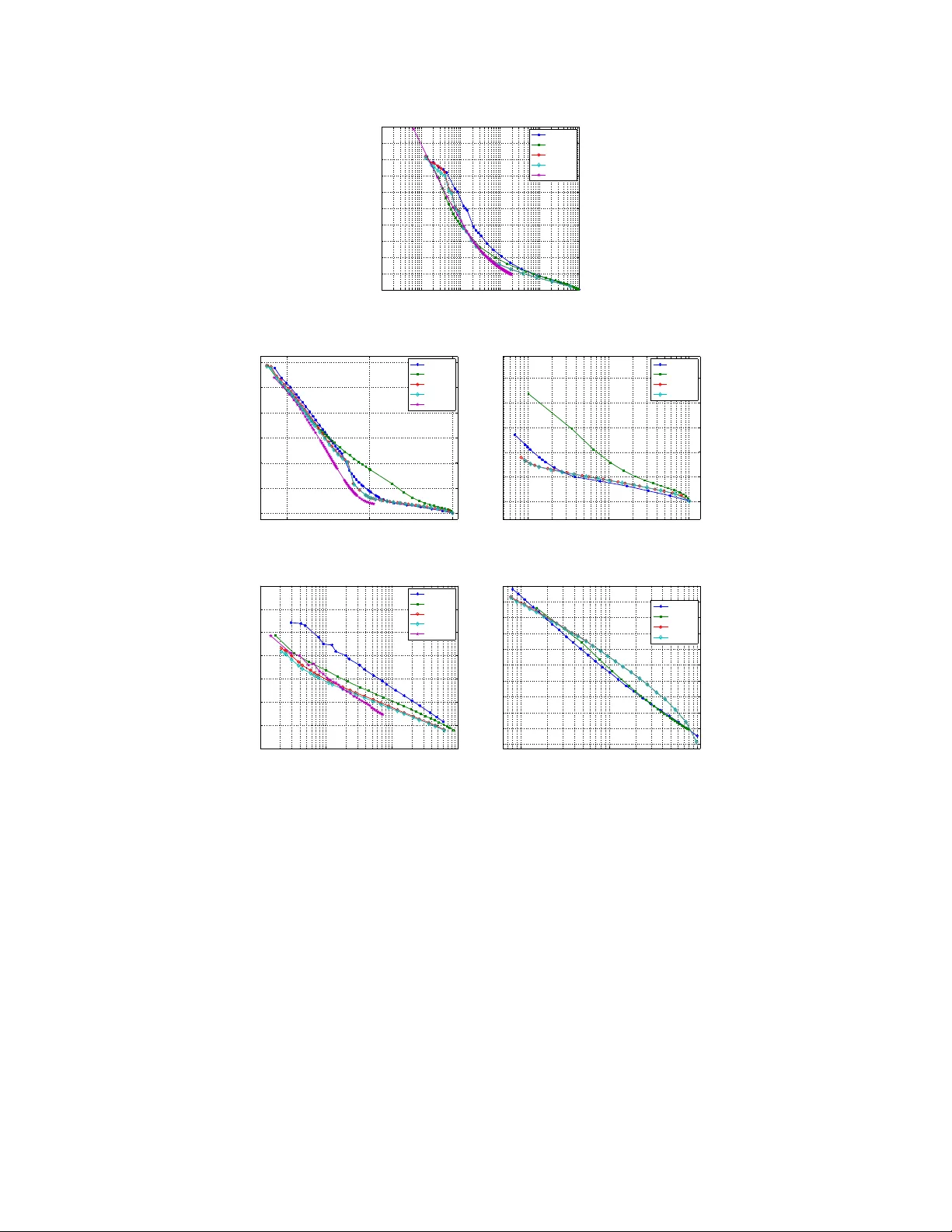
EXTENSION OF PCA TO HIGHER ORDER D A T A STR UCTURES: AN INTR ODUCTION TO TENSORS, TENSOR DECOMPOSITIONS, AND TENSOR PCA ALI ZARE, ALP OZDEMIR, MARK A. IWEN, AND SELIN A VIYENTE Abstract. The widespread use of multisensor technology and the emergence of big data sets hav e brough t the necessity to develop more versatile to ols to represent higher-order data with multiple asp ects and high dimensionalit y . Data in the form of multidimensional arrays, also referred to as tensors, arises in a v ariet y of applications including chemometrics, hypersp ectral imaging, high resolution videos, neuroimaging, biometrics, and so cial netw ork analysis. Early multiw ay data analysis approac hes reformatted such tensor data as large v ectors or matrices and then resorted to dimensionalit y reduction methods developed for classical t wo-w ay analysis suc h as PCA. Ho wev er, one cannot disco v er hidden components within m ultiw ay data using con v en tional PCA. T o this end, tensor decomp osition metho ds which are ﬂexible in the choice of the constraints and that extract more general laten t comp onen ts ha ve b een prop osed. In this pap er, we review the ma jor tensor decomp osition metho ds with a fo cus on problems targeted by classical PCA. In particular, w e presen t tensor metho ds that aim to solve three imp ortant challenges typically addressed by PCA: dimensionalit y reduction, i.e. lo w-rank tensor appro ximation, sup ervised learning, i.e. learning linear subspaces for feature extraction, and robust low-rank tensor reco v ery . W e also pro vide exp erimen tal results to compare diﬀerent tensor mo dels for both dimensionalit y reduction and sup ervised learning applications. Index T erms: PCA, T ensor, Multilinear Algebra, T ensor Decomp osition, T ensor PCA. 1. Introduction Principal Comp onent Analysis (PCA) is one of the oldest and widely used metho ds for dimen- sionalit y reduction in data science. The goal of PCA is to reduce the dimensionalit y of a data set, i.e. extract lo w-dimensional subspaces from high dimensional data, while preserving as muc h v ariability as possible [1]. Ov er the past decades, thanks to its simple, non-parametric nature, PCA has been used as a descriptiv e and adaptiv e exploratory method on n umerical data of v arious t ypes. Curren tly , PCA is commonly used to address three ma jor problems in data science: 1) Dimension- alit y reduction for large and high dimensional data sets, i.e. low-rank subspace appro ximation [2]; 2) Subspace learning for machine learning applications [3]; and 3) Robust low-rank matrix recov ery from missing samples or grossly corrupted data [4, 5]. How ever, these adv ances hav e b een mostly limited to v ector or matrix type data despite the fact that con tinued adv ances in information and sensing technology hav e b een making large-scale, multi-modal, and m ulti-relational datasets ever- more commonplace. Indeed, such m ultimo dal data sets are now commonly encoun tered in a h uge A. Zare (zareali@msu.edu) is with the Department of Computational Mathematics, Science and Engineering (CMSE), Mic higan State Universit y , East Lansing, MI, 48824, USA. A. Ozdemir (ozdemira@egr.msu.edu), and S. Aviyen te (aviy en te@egr.msu.edu) are with the Electrical and Com- puter Engineering, Mic higan State Universit y , East Lansing, MI, 48824, USA. Mark A. Iw en (markiw en@math.msu.edu) is with the Departmen t of Mathematics, and the Departmen t of Compu- tational Mathematics, Science and Engineering (CMSE), Michigan State Universit y , East Lansing, MI, 48824, USA. This w ork was supp orted in part by NSF CCF-1615489. v ariety of applications including c hemometrics [6], h yp erspectral imaging [7], high resolution videos [8], neuroimaging (EEG, fMRI) [9], biometrics [10, 11] and so cial net w ork analysis [12, 13]. When applied to these higher order data sets, standard vector and matrix mo dels such as PCA hav e b een sho wn to b e inadequate at capturing the cross-couplings across the diﬀeren t mo des and burdened b y the increasing storage and computational costs [14, 15, 16]. Therefore, there is a growing need for PCA type metho ds that can learn from tensor data while resp ecting its inherent multi-modal structure for multilinear dimensionality reduction and subspace estimation. The purp ose of this survey article is to introduce those who are well familiar with PCA metho ds for v ector type data to tensors with an eye tow ard discussing extensions of PCA and its v ariants for tensor type data. Although there are many excellen t review articles, tutorials and b o ok chap- ters written on tensor decomp osition (e.g. [15, 16, 17, 18, 19]), the fo cus of this review article is on extensions of PCA-based metho ds developed to address the current c hallenges listed ab ov e to tensors. F or example, [17] provides the fundamen tal theory and metho ds for tensor decomposi- tion/compression fo cusing on t w o particular mo dels, P ARAF A C and T uck er mo dels, without m uc h emphasis on tensor netw ork topologies, sup ervised learning and numerical examples that contrast the diﬀeren t mo dels. Similarly , [16] focuses on P ARAF A C and T uck er models with a special empha- sis on the uniqueness of the representations and computational algorithms to learn these mo dels from real data. Cic ho c ki et al. [19], on the other hand, mostly fo cus on tensor decomp osition metho ds for big data applications, providing an in depth review of tensor netw orks and diﬀerent net w ork top ologies. The current survey diﬀers from these in tw o key w a ys. First, the fo cus of the curren t surv ey is to in tro duce metho ds that can address the three main c hallenges or application areas that are currently b eing targeted by PCA for tensor t yp e data. Therefore, the current sur- v ey reviews dimensionality reduction and linear subspace learning metho ds for tensor t ype data as w ell as extensions of robust PCA to tensor t yp e data. Second, while the current surv ey attempts to giv e a comprehensiv e and concise theoretical o v erview of diﬀeren t tensor structures and repre- sen tations, it also pro vides exp erimen tal comparisons b et w een diﬀerent tensor structures for b oth dimensionalit y reduction and sup ervised learning applications. In order to accomplish these goals, w e review three main lines of researc h in tensor decomp ositions herein. First, we presen t methods for tensor decomp osition aimed at lo w-dimensional/lo w-rank appro ximation of higher order tensors. Early m ultiw a y data analysis relied on reshaping tensor data as a matrix and resorted to classical matrix factorization metho ds. How ev er, the matricization of tensor data cannot alw ays capture the in teractions and couplings across the diﬀeren t mo des. F or this reason, extensions of t w o-w a y matrix analysis tec hniques suc h as PCA, SVD and non- negativ e matrix factorization w ere developed in order to better address the issue of dimensionality reduction in tensors. After reviewing basic tensor algebra in Section 2, we then discuss these extensions in Section 3. In particular, we review the ma jor tensor representation mo dels including the CANonical DECOMPosition (CANDECOMP), also known as P ARAllel F A Ctor (P ARAF A C) mo del, the T uc k er, or multilinear singular v alue, decomp osition [20] and tensor net works, including the T ensor-T rain, Hierarc hical T uck er and other ma jor top ologies. These methods are discussed with resp ect to their dimensionality reduction capabilities, uniqueness and storage requirements. Section 3 concludes with an empirical comparison of several tensor decomp osition metho ds’ ability to compress several example datasets. Second, in Section 4, we summarize extensions of PCA and linear subspace learning methods in the con text of tensors. These include Multilinear Principal Comp onen t Analysis (MPCA), the T ensor Rank-One Decomp osition (TR OD), T ensor-T rain PCA (TT-PCA) and Hierarc hical T uc k er PCA (HT-PCA) metho ds which utilize the models in tro duced in Section 3 in order to learn a common subspace for a collection of tensors in a giv en training set. This common subspace is then used to pro ject test tensor samples in to low er-dimensional spaces and classify them [21, 22]. This framew ork has found applications in sup ervised learning settings, in particular for face and ob ject recognition images collected across diﬀerent mo dalities and 2 angles [23, 24, 25, 26]. Next, in Section 5, we address the issue of robust low-rank tensor recov ery for grossly corrupted and noisy higher order data for the diﬀerent tensor mo dels in tro duced in Section 3. Finally , in Section 6 w e pro vide an o v erview of ongoing w ork in the area of large tensor data factorization and computationally eﬃcien t implemen tation of the existing metho ds. 2. Not a tion, Tensor Basics, and Preludes to Tensor PCA Let [ n ] := { 1 , . . . , n } for all n ∈ N . A d -mo de , or d th-or der , tensor is simply a d -dimensional arra y of complex v alued data A ∈ C n 1 × n 2 ×···× n d for given dimension sizes n 1 , n 2 , . . . , n d ∈ N . Given this, each entry of a tensor is indexed b y an index vector i = ( i 1 , i 1 , . . . , i d ) ∈ [ n 1 ] × [ n 2 ] × · · · × [ n d ]. The entry of A indexed by i will alw a ys b e denoted by a ( i ) = a ( i 1 , i 2 , . . . , i d ) = a i 1 ,i 2 ,...,i d ∈ C . The j th en try p osition of the index v ector i for a tensor A will alw a ys b e referred to as the j th -mo de of A . In the remainder of this paper v ectors are alw ays b olded, matrices capitalized, tensors of order p oten tially ≥ 3 italicized, and tensor entries/scalars written in lo wer case. 2.1. Fib ers, Slices, and Other Sub-tensors. When encoun tered with a higher order tensor A it is often b eneﬁcial to lo ok for correlations across its diﬀeren t mo des. F or this reason, some of the many lo w er-order sub-tensors contained within any giv en higher-order tensor ha v e b een given sp ecial names and thereb y elev ated to special status. In this subsection w e will deﬁne a few of these. (a) (b) (c) Figure 1. T ensor, ﬁb ers and slices. (a) A 3-mo de tensor with a ﬁb er and slice. (b) Left: mo de-3 ﬁbers. Right: mo de-1 ﬁb ers. (c) mo de-3 slices. Fib ers are 1-mo de sub-tensors (i.e., sub-vectors) of a giv en d -mode tensor A ∈ C n 1 × n 2 ×···× n d . More sp eciﬁcally , a mo de- j ﬁb er of A is a 1-mo de sub-tensor indexed b y the j th mo de of A for an y giv en c hoices of j ∈ [ d ] and i ` ∈ [ n ` ] for all ` ∈ [ d ] \ { j } . Each such mo de- j ﬁb er is denoted b y (1) a ( i 1 , . . . , i j − 1 , : , i j +1 , . . . , i d ) = a i 1 ,...,i j − 1 , : ,i j +1 ,...,i d ∈ C n j . The k th en try of a mo de- j ﬁb er is a ( i 1 , . . . , i j − 1 , k , i j +1 , . . . , i d ) = a i 1 ,...,i j − 1 ,k,i j +1 ,...,i d ∈ C for each k ∈ [ n j ]. Note that there are Q k ∈ [ d ] \{ j } n k mo de- j ﬁb ers of an y given A ∈ C n 1 × n 2 ×···× n d . Example 1. Consider a 3 -mo de tensor A ∈ C m × n × p . Its mo de- 3 ﬁb er for any given ( i, j ) ∈ [ m ] × [ n ] is the 1 -mo de sub-tensor a ( i, j , :) = a i,j, : ∈ C p . Ther e ar e mn such mo de- 3 ﬁb ers of A . Fib ers of a 3 -mo de tensor A ∈ C 3 × 4 × 5 ar e depicte d in Figur e 1(b). In this pap er slic es , will alwa ys b e ( d − 1)-mode sub-tensors of a given d -mo de tensor A ∈ C n 1 × n 2 ×···× n d . In particular, a mo de- j slic e of A is a ( d − 1)-mo de sub-tensor indexed by all but the j th mo de of A for an y giv en choice of j ∈ [ d ]. Each suc h mo de- j slice is denoted b y (2) A i j = k = A (: , . . . , : , k , : , . . . , :) = A : ,..., : ,k, : ,..., : ∈ C n 1 ×···× n j − 1 × n j +1 ×···× n d for an y choice of k ∈ [ n j ]. The ( i 1 , . . . , i j − 1 , i j +1 , . . . , i d ) th en try of a mo de- j slice is (3) ( a i j = k )( i 1 , . . . , i j − 1 , i j +1 , . . . , i d ) = a ( i 1 , . . . , i j − 1 , k , i j +1 , . . . , i d ) = a i 1 ,...,i j − 1 ,k,i j +1 ,...,i d ∈ C 3 for eac h ( i 1 , . . . , i j − 1 , i j +1 , . . . , i d ) ∈ [ n 1 ] × · · · × [ n j − 1 ] × [ n j +1 ] × · · · × [ n d ]. It is easy to see that there are alwa ys just n j mo de- j slices of an y giv en A ∈ C n 1 × n 2 ×···× n d . Example 2. Consider a 3 -mo de tensor A ∈ C m × n × p . Its mo de- 3 slic e for any given k ∈ [ p ] is the 2 -mo de sub-tensor (i.e., matrix) A i 3 = k = A (: , : , k ) = A : , : ,k ∈ C m × n . Ther e ar e p such mo de- 3 slic es of A . In Figur e 1(c), the 5 mo de- 3 slic es of A ∈ C 3 × 4 × 5 c an b e viewe d. 2.2. T ensor V ectorization, Flattening, and Reshaping. There are a tremendous m ultitude of w ays one can reshap e a d -mo de tensor into another tensor with a diﬀerent num b er of modes. P erhaps most imp ortan t among these are the transformation of a given tensor A ∈ C n 1 × n 2 ×···× n d in to a v ector or matrix so that metho ds from standard n umerical linear algebra can b e applied to the reshaped tensor data thereafter. The ve ctorization of A ∈ C n 1 × n 2 ×···× n d will alw a ys reshap e A into a v ector (i.e., 1st-order tensor) denoted by a ∈ C n 1 n 2 ··· n d . This pro cess can b e accomplished n umerically by , e.g., recursiv ely v ectorizing the last tw o mo des of A (i.e., each matrix A ( i 1 , . . . , i d − 2 , : , :)) according to their ro w- ma jor order un til only one mode remains. When done in this fashion the en tries of the v ectorization a can b e rapidly retrieved from A via the formula (4) a j = A ( g 1 ( j ) , . . . , g d ( j )) , where eac h of the index functions g m : [ n 1 n 2 · · · n d ] → [ n m ] is deﬁned for all m ∈ [ d ] b y (5) g m ( j ) := & j Q ` ∈ [ d ] \ [ m ] n ` ' mo d n m + 1 . Herein we will alw a ys use the con ven tion that Q ` ∈∅ n ` := 1 to handle the case where, e.g., [ d ] \ [ m ] is the empty set ab o v e. The pro cess of reshaping a ( d > 2)-mo de tensor in to a matrix is kno wn as matricizing , ﬂattening , or unfolding , the tensor. There are 2 d − 2 nontrivial wa ys in which one may create a matrix from a d -mo de tensor by partitioning its d mo des into t w o diﬀeren t “ro w” and “column” subsets of mo des (eac h of which is then implicitly vectorized separately). 1 The most often considered of these are the mo de- j v ariants mentioned below (excluding, p erhaps, the alternate matricizations utilized as part of, e.g., the tensor train [27] and hierarchical SVD [28] decomposition metho ds.) The mo de- j matricization , mo de- j ﬂattening , or mo de- j unfolding of a tensor A ∈ C n 1 × n 2 ×···× n d , denoted by A ( j ) ∈ C n j × Q ` ∈ [ d ] \{ j } n ` , is a matrix whose columns consist of all the mo de- j ﬁb ers of A . More explicitly , A ( j ) is determined herein by deﬁning its en tries to b e (6)  a ( j )  k,l := A ( h 1 ( l ) , h 2 ( l ) , . . . , h j − 1 ( l ) , k , h j +1 ( l ) , . . . , h d − 1 ( l ) , h d ( l )) , where, e.g., the index functions h m : h Q ` ∈ [ d ] \{ j } n ` i → [ n m ] are deﬁned by (7) h m ( l ) := & l Q ` ∈ [ d ] \ ([ m ] ∪{ j } ) n ` ' mo d n m + 1 for all m ∈ [ d ] \ { j } and l ∈ Q ` ∈ [ d ] \{ j } n ` . Note that A ( j ) ’s columns are ordered b y v arying the index of the largest non- j mode ( d unless a mo de- d unfolding is b eing constructed) fastest, follo w ed b y v arying the second largest non- j mo de second fastest, etc.. In Figure 2, the mo de-1 matricization of A ∈ C 3 × 4 × 5 is formed in this w ay using its mode-1 ﬁb ers. 1 One can use Stirling num b ers of the second kind to easily enumerate all p ossible mo de partitions. 4 Figure 2. F ormation of the mode-1 unfolding (b elo w) using the mo de-1 ﬁb ers of a 3-mode tensor (ab o v e). Example 3. As an example, c onsider a 3 -mo de tensor A ∈ C n 1 × n 2 × n 3 . Its mo de- 1 matricization is (8) A (1) = h ( A i 2 =1 ) (1)    ( A i 2 =2 ) (1)    . . .    ( A i 2 = n 2 ) (1) i ∈ C n 1 × n 2 n 3 wher e ( A i 2 = c ) (1) ∈ C n 1 × n 3 is the mo de- 1 matricization of the mo de- 2 slic e of A at i 2 = c for e ach c ∈ [ n 2 ] . Note that we stil l c onsider e ach mo de- 2 slic e A i 2 = c to b e indexe d by i 1 and i 3 ab ove. As a r esult, e.g., ( A i 2 =1 ) (3) wil l b e c onsider e d me aningful while ( A i 2 =1 ) (2) wil l b e c onsider e d me aningless in the same way that, e.g., ( A i 2 =1 ) (100) is me aningless. That is, even though A i 2 = c only has two mo des, we wil l stil l c onsider them to b e its “ﬁrst” and “thir d” mo des (i.e., its two mo de p ositions ar e stil l indexe d by 1 and 3 , r esp e ctively). Though p otential ly c ounterintuitive at ﬁrst, this notational c onvention wil l simplify the interpr etation of expr essions like (8) – (10) going forwar d. Given this c onvention, we also have that (9) A (2) = h ( A i 1 =1 ) (2)    ( A i 1 =2 ) (2)    . . .    ( A i 1 = n 1 ) (2) i ∈ C n 2 × n 1 n 3 , and (10) A (3) = h ( A i 1 =1 ) (3)    ( A i 1 =2 ) (3)    . . .    ( A i 1 = n 1 ) (3) i ∈ C n 3 × n 1 n 2 . 2.3. The Standard Inner Product Space of d -mo de T ensors. The set of all d th-order tensors A ∈ C n 1 × n 2 ×···× n d forms a vector space o v er the complex num b ers when equipped with comp onen- t wise addition and scalar m ultiplication. This v ector space is usually endo w ed with the Euclidean inner pro duct. More sp eciﬁcally , the inner pro duct of A , B ∈ C n 1 × n 2 × ... × n d will alwa ys be giv en by (11) hA , B i := n 1 X i 1 =1 n 2 X i 2 =1 . . . n d X i d =1 a ( i 1 , i 2 , . . . , i d ) b ( i 1 , i 2 , . . . , i d ) , where ( · ) denotes the complex conjugation operation. This inner pro duct then giv es rise to the standard Euclidean norm (12) kAk := p hA , Ai = v u u t n 1 X i 1 =1 n 2 X i 2 =1 . . . n d X i d =1 | a ( i 1 , i 2 , . . . , i d ) | 2 . If hA , B i = 0 we will say that A and B are ortho gonal . If A and B are orthogonal and also hav e unit norm (i.e., hav e kAk = kB k = 1) we will sa y that they are orthonormal . 5 It is w orth noting that trivial inner pro duct preserving isomorphisms exist betw een this standard inner pro duct space and any of its reshap ed versions (i.e., reshaping can b e view ed as an isomor- phism b et w een the original d -mo de tensor v ector space and its reshap ed target vector space). In particular, the pro cess of reshaping tensors is linear. If, for example, A , B ∈ C n 1 × n 2 × ... × n d then one can see that the mo de- j unfolding of A + B ∈ C n 1 × n 2 × ... × n d is ( A + B ) ( j ) = A ( j ) + B ( j ) for all j ∈ [ d ]. Similarly , the vectorization of A + B is alwa ys exactly a + b . 2.4. T ensor Pro ducts and j -Mo de Pro ducts. It is o ccasionally desirable to build one’s o wn higher order tensor using t w o low er order tensors. This is particularly true when one builds them up using v ectors as part of, e.g., P ARAF AC/CANDECOMP decomp osition techniques [29, 30, 31, 32, 33]. T o w ard this end we will utilize the tensor pr o duct of tw o tensors A ∈ C n 1 × n 2 ×···× n d and B ∈ C n 0 1 × n 0 2 ×···× n 0 d 0 . The result of the tensor pro duct, A ⊗ B ∈ C n 1 × n 2 ×···× n d × n 0 1 × n 0 2 ×···× n 0 d 0 , is a ( d + d 0 )-mo de tensor whose en tries are giv en by (13) ( A ⊗ B ) i 1 ,...,i d ,i 0 1 ,...,i 0 d 0 = a ( i 1 , . . . , i d ) b ( i 0 1 , . . . , i 0 d 0 ) . A d th-order tensor whic h is built up from d vectors using the tensor pro duct is called a r ank- 1 tensor . F or example, N 4 k =1 a k = a 1 ⊗ a 2 ⊗ a 3 ⊗ a 4 ∈ C n 1 × n 2 × n 3 × n 4 is a rank-1 tensor with 4 mo des whic h is built from a 1 ∈ C n 1 , a 2 ∈ C n 2 , a 3 ∈ C n 3 , and a 4 ∈ C n 4 . Note that this 4th-order tensor is unam biguously called “rank-1” due to the fact that a 1 ⊗ a 2 ⊗ a 3 ⊗ a 4 ∈ C n 1 × n 2 × n 3 × n 4 is b oth built up from rank-1 tensors, and b ecause every mode- j unfolding of a 1 ⊗ a 2 ⊗ a 3 ⊗ a 4 is also a rank-1 matrix. Finally , the mo de- j pr o duct of d -mo de tensor A ∈ C n 1 ×···× n j − 1 × n j × n j +1 ×···× n d with a matrix U ∈ C m j × n j is another d -mo de tensor A × j U ∈ C n 1 ×···× n j − 1 × m j × n j +1 ×···× n d . Its entries are given b y (14) ( A × j U ) i 1 ,...,i j − 1 ,`,i j +1 ,...,i d = n j X i j =1 a i 1 ,...,i j ,...,i d u `,i j for all ( i 1 , . . . , i j − 1 , `, i j +1 , . . . , i d ) ∈ [ n 1 ] × · · · × [ n j − 1 ] × [ m j ] × [ n j +1 ] × · · · × [ n d ]. Lo oking at the mo de- j unfoldings of A × j U and A one can easily see that ( A × j U ) ( j ) = U A ( j ) holds for all j ∈ [ d ]. Mo de- j pro ducts pla y a particularly imp ortant role in man y tensor PCA and tensor factorization metho ds [34, 20, 23, 33]. F or this reason it is worth stating some of their basic properties: mainly , mo de- j pro ducts are bilinear, commute on diﬀerent mo des, and combine in reverse order on the same mode. The follo wing simple lemma formally lists these imp ortant prop erties. Lemma 1. L et A , B ∈ C n 1 × n 2 ×···× n d , α, β ∈ C , and U ` , V ` ∈ C m ` × n ` for al l ` ∈ [ d ] . The fol lowing four pr op erties hold: ( † ) ( α A + β B ) × j U j = α ( A × j U j ) + β ( B × j U j ) . ( †† ) A × j ( αU j + β V j ) = α ( A × j U j ) + β ( A × j V j ) . ( † † † ) If j 6 = ` then A × j U j × ` V ` = ( A × j U j ) × ` V ` = ( A × ` V ` ) × j U j = A × ` V ` × j U j . ( † † †† ) If W ∈ C p × m j then A × j U j × j W = ( A × j U j ) × j W = A × j ( W U j ) = A × j W U j . Another w ay to represent tensor pro ducts is to deﬁne index contractions. An index c ontr action is the sum o v er all the p ossible v alues of the rep eated indices of a set of tensors. F or example, the ma- trix pro duct C αγ = P D β =1 A αβ B β γ can b e thought of the con traction of index β . One can also con- sider tensor pro ducts through index contractions suc h as F γ ω ρσ = P D α,β ,δ,ν,µ =1 A αβ δ σ B β γ µ C δ ν µω E ν ρα , where the indices α, β , δ, ν, µ are con tracted to produce a new four-mo de tensor. The representation 6 of a tensor through the contraction of indices of other tensors will b e particularly imp ortan t for the study of tensor net works (TNs). 3. Tensor F actoriza tion and Compression Methods In this section, we focus on tensor decomp osition metho ds that provide lo w-rank approximations for m ultilinear datasets by reducing their complexity similar to the wa y PCA/SVD do es for matri- ces. Adv an tages of using multiw a y analysis ov er t w o-w ay analysis in terms of uniqueness, robustness to noise, and computational complexity hav e b een shown in man y studies (see, e.g., [18, 35, 36]). In this section w e review some of the most commonly used tensor mo dels for represen tation and compression and presen t results on their uniqueness and storage complexities. W e then empirically ev aluate the compression versus approximation error p erformance of sev eral of these metho ds for three diﬀeren t higher order datasets. 3.1. CANDECOMP/P ARAF A C Decomp osition (CPD). CPD is a generalization of PCA to higher order array and represents a d -mo de tensor X ∈ R n 1 × n 2 × ... × n d as a combination of rank-one tensors [37]. (15) X = R X r =1 λ r a (1) r ⊗ a (2) r ⊗ .... ⊗ a ( d ) r , where R is a p ositiv e integer, λ r is the w eigh t of the r th rank-one tensor, a ( i ) r ∈ R n i is the r th factor of i th mo de with unit norm where i ∈ [ d ] and r ∈ [ R ]. Alternatively , X can b e represented as mo de products of a diagonal core tensor S with en tries s ( i, i, ..., i ) = λ i and factor matrices A ( i ) = [ a ( i ) 1 a ( i ) 2 ... a ( i ) R ] for i ∈ [ d ]: (16) X = S × 1 A (1) × 2 A (2) ... × d A ( d ) . The main restriction of the P ARAF AC mo del is that the factors across diﬀerent mo des only interact factorwise. F or example, for a 3-mo de tensor, the i th factor corresp onding to the ﬁrst mo de only in teracts with the i th factors of the second and third modes. Rank-R approximation of a d th-order tensor X ∈ R n 1 × n 2 ... × n d with n 1 = n 2 = . . . = n d = n obtained b y CPD is represented using O ( Rdn ) parameters, which is less than the num b er of parameters required for PCA applied to an unfolded matrix. Uniqueness : In a recen t review article, Sidirop oulos et al. [16] pro vided t wo alternative pro ofs for the uniqueness of the P ARAF AC model. Given a tensor X of rank R , its P ARAF AC decomposition is essen tially unique, i.e. the factor matrices A (1) , . . . , A ( d ) are unique up to a common p ermutation and scaling of columns for the given num b er of terms. Alternativ ely , Krusk al provided results on uniqueness of 3-mo de CPD depending on matrix k -rank as: (17) k A (1) + k A (2) + k A (3) ≥ 2 R + 2 , where k A ( i ) is the maxim um v alue k such that any k columns of A ( i ) are linearly indep enden t [37]. This result is later generalized for d -mode tensors in [38] as: (18) d X i =1 k A ( i ) ≥ 2 R + d − 1 . Under these conditions, the CPD solution is unique and the estimated model cannot be rotated without a loss of ﬁt. Computational Issues : CPD is most commonly computed b y alternating least squares (ALS) b y successively assuming the factors in d − 1 modes kno wn and then estimating the unkno wn set of parameters of the last mo de. F or each mo de and each iteration, the F rob enious norm of 7 the diﬀerence b et w een input tensor and CPD appro ximation is minimized. ALS is an attractive metho d since it ensures the improv emen t of the solution in ev ery iteration. How ever, in practice, the existence of large amount of noise or the high order of the mo del may preven t ALS to conv erge to global minima or require sev eral thousands of iterations [33, 15, 39]. Diﬀerent metho ds hav e b een proposed to impro v e p erformance and accelerate conv ergence rate of CPD algorithms [40, 41]. A n um b er of particular tec hniques exist, such as line searc h extrapolation metho ds [42, 43, 44] and compression [45]. Instead of alternating estimation, all-at-once algorithms such as the OPT algorithm [46], the conjugate gradien t algorithm for nonnegative CP [47], the PMF3, damp ed Gauss-Newton (dGN) algorithms [48] and fast dGN [49] ha v e been studied to deal with problems of a slow conv ergence of the ALS in some cases. Another approach is to consider the CP decomp osition as a joint diagonalization problem [50, 51]. 3.2. T uc k er Decomp osition and HoSVD. T uc k er decomp osition is a natural extension of the SVD to d -mo de tensors and decomposes the tensor in to a core tensor m ultiplied b y a matrix along eac h mode [52, 15, 39]. T uck er decomp osition of a d -mo de tensor X ∈ R n 1 × n 2 × ... × n d is w ritten as: (19) X = P n 1 i 1 =1 ... P n d i d =1 s i 1 ,i 2 ,...,i d  u (1) i 1 ⊗ u (2) i 2 ⊗ ... ⊗ u ( d ) i d  , X = S × 1 U (1) × 2 U (2) ... × d U ( d ) , where the matrices U ( i ) = [ u ( i ) 1 u ( i ) 2 ... u ( i ) n d ]s are square factor matrices and the core tensor S is obtained by S = X × 1 U (1) , > × 2 U (2) , > ... × d U ( d ) , > , where U ( i ) , > denotes the transp ose of the factor matrix along each mo de. It is common for the T uc k er decomp osition to assume the rank of U ( i ) s to b e less than n i so that S is a compression of X . Multilinear-rank-R appro ximation of a d th-order tensor X ∈ R n 1 × n... × n d with n 1 = n 2 = . . . = n d = n is represented using O ( Rnd + R d ) parameters in the T uc k er mo del. In contrast to P ARAF AC, T uck er mo dels allo w interactions b etw een the factors obtained across the mo des and the core tensor includes the strength of these in teractions. In summary , both CPD and T uck er are sum-of-outer pro ducts mo dels, and one can argue that the most general form of one con tains the other. How ev er, what distinguishes the t w o is uniqueness. Uniqueness: As it can b e seen in (19), one can linearly transform the columns of U ( i ) and absorb the inv erse transformation in the core tensor S . The subspaces deﬁned by the factor matrices in T uck er decomp osition are unique, while the bases in these subspaces ma y b e c hosen arbitrarily – their c hoice is comp ensated for within the core tensor. F or this reason, the T uc k er mo del is not unique unless additional constraints are placed on U ( i ) s and/or the core tensor. Constrain ts such as orthogonalit y , nonnegativ eness, sparsit y , indep endence and smo othness hav e been imp osed on the factor matrices to obtain unique decompositions [53, 54, 55, 56]. The Higher Order SVD (HoSVD) is a sp ecial case of T uc ker decomp osition obtained b y adding an orthogonalit y constrain t to the component matrices. In HoSVD, the factor matrices, U ( i ) s, are the left singular v ectors of eac h ﬂattening X ( i ) . In HoSVD, lo w n-rank approximation of X can be obtained b y truncating the orthogonal factor matrices of HoSVD resulting in truncated HoSVD. Due to the orthogonality of the core tensor, HoSVD is unique for a sp eciﬁc m ultilinear rank. As opp osed to the SVD for matrices, the ( R 1 , R 2 , . . . , R d ) truncation of the HoSVD is not the best ( R 1 , R 2 , . . . , R d ) appro ximation of X . The b est ( R 1 , R 2 , . . . , R d ) − rank appro ximation is obtained b y solving the following optimization problem. (20) min S ,U (1) ,U (2) ,...,U ( d )   X − S × 1 U (1) × 2 U (2) . . . × d U ( d )   sub ject to S ∈ R R 1 × R 2 × ... × R d , U ( i ) ∈ R n i × R i and column wise orthogonal for all i ∈ [ d ] . 8 Computational Issues: It has b een shown that this optimization problem can b e solved by the ALS approac h iteratively and the metho d is known as higher-order orthogonal iteration (HOOI) [52]. F or man y applications, HoSVD is considered to b e suﬃciently go od, or it can serv e as an initial v alue in algorithms for ﬁnding the best approximation [57]. T o identify hidden nonnegativ e patterns in a tensor, nonnegative matrix factorization algorithms ha v e b een adapted to T uc k er mo del [56, 58, 59, 60, 53]. NTD of a tensor X ∈ R n 1 × n 2 × ... × n d can b e obtained by solving: (21) min S ,U (1) ,U (2) ,...,U ( d )   X − S × 1 U (1) × 2 U (2) . . . × d U ( d )   sub ject to S ∈ R R 1 × R 2 × ... × R d + , U ( i ) ∈ R n i × R i + ; i ∈ [ d ] . This optimization problem can b e solved using nonnegativ e ALS and up dating the core tensor S and factor matrices U ( i ) at each iteration dep ending on diﬀerent up dating rules suc h as alpha and beta divergences [60, 59] or lo w-rank NMF [56, 54]. 3.3. T ensor Net works. T ensor decomp ositions such as P ARAF AC and T uck er decomp ose com- plex high dimensional data tensors into their factor tensors and matrices. T ensor net w orks (TNs), on the other hand, represent a higher-order tensor as a set of sparsely in terconnected low er-order tensors, t ypically 3rd-order and 4th-order tensors called core and pro vide computational and stor- age b eneﬁts [61, 14, 19]. More formally , a TN is a se t of tensors where some, or all, of its indices are contracted according to some pattern. The contraction of a TN with some op en indices results in another tensor. One imp ortan t prop ert y of TN is that the total num b er of op erations that must b e done to obtain the ﬁnal result of a TN contraction dep ends on the order in which indices in the TN are con tracted, i.e., for a given tensor there are many diﬀerent TN represen tations and ﬁnding the optimal order of indices to b e contracted is a crucial step in the eﬃciency of TN decomp osition. The optimized top ologies yield simpliﬁed and con v enien t graphical representations of higher-order tensor data [62, 63]. Some commonly encoun tered tensor net work top ologies include Hierarc hical T uck er (HT), T ree T ensor Net work State (TTNS), T ensor T rain (TT) and tensor net works with cycles such as Pro jected En tangled Pair States (PEPS) and Pro jected En tangled Pair Op erators (PEPO). Uniqueness: As noted ab o v e, for a given tensor there are many diﬀerent TN represen tations, so in general, there is not a unique representation. The uniqueness of v arious TN mo dels under diﬀerent constrain ts is still an active ﬁeld of researc h [19]. 3.3.1. Hier ar chic al T ensor De c omp osition. T o reduce the memory requirements of T uc k er decom- p osition, hierarc hical T uc k er (HT) decomp osition (also called hierarc hical tensor represen tation) has been prop osed [64, 28, 39]. Hierarc hical T uck er Decomp osition recursively splits the modes based on a hierarch y and creates a binary tree T containing a subset of the mo des t ⊂ [ d ] at each no de [28]. F actor matrices U t s are obtained from the SVD of X ( t ) whic h is the matricization of a tensor X corresp onding to the subset of the mo des t at eac h no de. How ever, this matricization is diﬀerent from mo de-n matricization of the tensor, and rows of X ( t ) corresp ond to the mo des in the set of t while columns of X ( t ) store indices of the remaining mo des. Constructed tree structure yields hierarc h y amongst the factor matrices U t whose columns span X ( t ) for eac h t . Let t 1 and t 2 b e children of t . F or t = t 1 ∪ t 2 and t 1 ∩ t 2 = ∅ , there exists a transfer matrix B t suc h that U t = ( U t 1 ⊗ U t 2 ) B t , where B t ∈ R R t 1 R t 2 × R t . By assuming R t = R , HT-rank-R appro ximation of X ∈ R n 1 × n 2 × ... × n d with n 1 = n 2 = . . . = n d = n requires storing U t s for the leaf nodes and B t s for the other no des in T with O ( dnR + dR 3 ) parameters [39]. 9 3.3.2. T ensor T r ain De c omp osition. T ensor T rain (TT) Decomp osition can b e interpreted as a sp ecial case of the HT, where all no des of the underlying tensor netw ork are connected in a cascade or train. It has b een prop osed to compress large tensor data in to smaller core tensors [27]. This mo del allo ws users to av oid the exp onen tial growth of T uck er mo del and provides more eﬃcient storage complexit y . TT decomp osition of a tensor X ∈ R n 1 × n 2 × ... × n d is written as: (22) X i 1 ,...i d = G 1 ( i 1 ) · G 2 ( i 2 ) · · · G d ( i d ) , where G m ( i m ) ∈ R R m − 1 × R m is the i m th lateral slice of the core G m ∈ R R m − 1 × n m × R m , R m s b eing the TT-rank with R 0 = R d = 1. Computational Issues: TT decomp osition of X is obtained through a sequence of SVDs. First, G 1 is obtained from SVD of mo de-1 matricization of X as (23) X (1) = U S V > where G 1 = U ∈ R n 1 × M 1 and r ank ( U ) = R 1 ≤ n 1 . Note that, S V > ∈ R R 1 × n 2 n 3 ...n d . Let W ∈ R R 1 n 2 × n 3 ...n d b e a reshap ed version of S V > . Then, G 2 ∈ R R 1 × n 2 × R 2 is obtained b y reshaping left-singular v ectors of W , where W = U S V > and U ∈ R R 1 n 2 × R 2 , r ank ( U ) = R 2 ≤ r ank ( W ) and S V > ∈ R R 2 × n 3 ...n d . By rep eating this pro cedure, all of the core tensors G i s are obtained by a sequence of SVD decomp ositions of sp eciﬁc matricizations of X . The storage complexity of TT- rank-R appro ximation of a d th-order tensor X ∈ R n 1 × n 2 ... × n d with n 1 = n 2 = . . . = n d = n is O ( dnR 2 ). It is imp ortan t to note that the TT format is kno wn as the Matrix Pro duct State (MPS) rep- resen tation with the Op en Boundary Conditions (OBC) in the quan tum physics communit y [61]. Some of the adv antages of the TT/MPS mo del ov er HT are its simpler practical implementation as no binary tree needs to b e determined, the simplicity of the computation, computational eﬃciency (linear in the tensor order). Although TT format has b een used widely in signal pro cessing and machine learning, it suﬀers from a couple of limitations. First, TT mo del requires rank-1 constraints on the b order factors, i.e. they ha v e to be matrices. Second and most imp ortantly , the multiplications of the TT cores are not p erm utation in v ariant requiring the optimization of the ordering using pro cedures such as mutual information estimation [65, 66]. These drawbac ks hav e b een recently addressed by the tensor ring (TR) decomp osition [67, 68]. TR decomp osition remov es the unit rank constrain ts for the boundary cores and utilizes a trace op eration in the decomp osition, which remov es the dep endency on the core order. 3.4. T ensor Singular V alue Decomp osition (t-SVD). t-SVD is deﬁned for 3rd order tensors based on t-pro duct [69]. Algebra b ehind t-SVD is diﬀerent than regular m ultilinear algebra and dep ends on linear operators deﬁned on third-order tensors. In this approac h, third-order tensor X ∈ R n 1 × n 2 × n 3 is decomposed as (24) X = U ∗ S ∗ V T , where U ∈ R n 1 × n 1 × n 3 and V ∈ R n 2 × n 2 × n 3 are orthogonal tensors with resp ect to the 0 ∗ 0 op eration, S n 1 × n 2 × n 3 is a tensor whose rectangular frontal slices are diagonal, and the entries in S are called the singular v alues of X . 0 ∗ 0 denotes the t-pro duct and deﬁned as the circular con v olution b et w een mo de-3 ﬁbers of same size. One can obtain this decomp osition by computing matrix SVDs in the F ourier domain. t-SVD deﬁnes the notion of tubal rank, where the tubal rank of X is deﬁned to b e the n um b er of non-zero singular tub es of S . Moreov er, unlik e CPD and T uc ker mo dels, truncated t-SVD with a given rank can b e sho wn b e the optimal appro ximation in terms of minimizing the F rob enius norm of the error. rank-R approximation of X ∈ R n 1 × n 2 × n 3 can b e represented using O ( Rn 3 ( n 1 + n 2 + 1)) entries. 10 3.5. An Empirical Comparison of Diﬀerent T ensor Decomp osition Metho ds. In this section the CANDECOMP/P ARAF A C, T uck er (HOOI), HoSVD, HT, and TT decomp ositions are compared in terms of data reduction rate and normalized reconstruction error. The data sets used for this purp ose are: (1) PIE data set: This database con tains 138 images taken from one individual under diﬀeren t illumination conditions and from 6 diﬀerent angles [70]. All 244 × 320 images of the individual form a 3-mode tensor X ∈ R 244 × 320 × 138 . (2) Hyp ersp e ctr al Image (HSI) data set: This database contains 100 images tak en at 148 wa v elengths [71]. Images consist of 801 × 1000 pixels, forming a 3-mo de tensor X ∈ R 801 × 1000 × 148 . (3) COIL-100 data set: This database includes 7200 images tak en from 100 ob jects [72]. Eac h ob ject w as imaged at 72 diﬀeren t angles separated b y 5 degrees, resulting in 72 images p er ob ject, eac h one consisting of 128 × 128 pixels. The original database is a 128 × 128 × 7200 tensor whic h w as reshaped as a 4-mo de tensor X ∈ R 128 × 128 × 72 × 100 for the exp eriments. Sample images from the ab o v e data sets can b e viewed in Figure 3. 100 200 300 400 500 600 50 100 150 200 (a) 100 200 300 400 500 600 700 800 900 1000 100 200 300 400 500 600 700 800 (b) (c) Figure 3. Sample images from data sets used in exp erimen ts. (a) The PIE data set. (b) The Hypersp ectral Image. (c) The COIL-100 data set. Sev eral soft ware pac k ages were used to generate the results. The T uc k er (HOOI) and CPD metho ds were ev aluated using the T ensorL ab pack age [73]. F or CPD, the structure detection and exploitation option w as disabled in order to a v oid complications on the larger datasets ( COIL-100 and HSI ). 2 F or CPD, the n um b er of rank-1 tensors in the decomp osition, R , is given as the input parameter to ev aluate the appro ximation error with resp ect to compression rate. F or HOOI, the input is a cell array of factor matrices for diﬀeren t modes that are used as initialization for the main algorithm. T o generate the initial factor matrices, HoSVD w as computed with the TP T o ol [74]. The original version of the co de w as slightly mo diﬁed in a wa y that the input parameter to HoSVD is the threshold 0 ≤ τ ≤ 1 deﬁned in (25), where n 0 is the minimum num ber of singular v alues that allow the inequality to hold for mo de i . The same threshold v alue, τ , was chosen for 2 T o disable the structure exploitation option, the ﬁeld options.ExploitStructur e w as set to false in cp d.m. The large-scale memory threshold was also changed from 2 GB to 16 GB in mtkrprod.m to preven t the large intermediate solutions from causing memory issues. 11 all modes. (25) n 0 P k =1 σ k n i P k =1 σ k ≥ τ . The T ensor-T r ain T o olb ox [75] w as used to generate results for the T ensor-T rain (TT) metho d. The input parameter for TT is the accuracy (error) with which the data should b e stored in the T ensor-T rain format. Similarly , the Hier ar chic al T ucker T o olb ox [76] w as used to generate results for the Hierarchical T uck er (HT) metho d. The input parameter for HT is the maximal hierarchical rank. The diﬀeren t ranges of input parameters for eac h metho d hav e b een summarized in T able 1. These parameters hav e b een chosen to yield comparable reconstruction errors and compression rates across diﬀerent metho ds. The experimental results are given in Figure 4. Here, compression is deﬁned as the ratio of size of the output data to the size of input data. 3 The relativ e error was calculated using (26) E = k input − output k k input k , where input denotes the input tensor and output denotes the (compressed) tensor reconstructed using the given metho d. T able 1. Range of input parameter v alues used for the diﬀerent metho ds to gen- erate the results shown in Figure 4. Data PIE HSI COIL-100 Figure 5(a) 5(b) 5(c) 5(d) 5(e) TT (error) 0.001-0.5 0.001-0.5 0.001-0.0555 0.21-0.5 0.0831-0.2 HT (max. H. rank) 2-300 2-960 100-960 1-80 100-3500 HoSVD (threshold τ ) 0.2-0.99 0.15-0.9999 0.8841-0.9999 0.4-0.76 0.77-0.999 HOOI (threshold τ ) 0.2-0.99 0.15-0.9999 0.8864-0.9999 0.4-0.76 0.77-0.999 CPD (rank R ) 1-300 3-767 - 4-200 - The following observ ations can b e made from Figure 4. CPD has diﬃculty conv erging when the input rank parameter, R , is large especially for larger data sets. How ev er, it provides the b est compression p erformance when it con v erges. F or the PIE data set, HT and sp eciﬁcally TT do not p erform w ell for most compression ranges. How ever, HT outp erforms the other metho ds with resp ect to appro ximation error for compression rates b elo w 10 − 2 . F or the HSI data set, TT and HT again do not p erform very w ell, particularly for compression v alues around 10 − 2 . HT con tin ues to p erform po orly for larger compression rates as well. F or the COIL-100 data set, TT and HT generate v ery go o d results for compression rates ab o v e 10 − 2 , but fail to do so for low er compression rates. This is esp ecially the case for TT. It should b e noted that the largest num ber of mo des for the tensors considered in this pap er is only 4. T ensor netw ork mo dels such as TT and HT are exp ected to perform b etter for higher n um b er of mo des. HoSVD and HOOI pro vide very similar results in all data sets, with HOOI performing slightly b etter. They generally app ear to pro vide the b est compression versus error results of all the metho ds in regimes where CPD do es not w ork well, with the exception of the COIL dataset where HT and TT outp erform them at higher compression rates. 3 No other data compression metho ds were used to help reduce the size of the data. Data size was compared in terms of bytes needed to represen t each metho d’s output v ersus its input. When the same precision is used for all data, this is equal to measuring the total num b er of elements of the input and output arrays. 12 10 −5 10 −4 10 −3 10 −2 10 −1 10 0 0 0.05 0.1 0.15 0.2 0.25 0.3 0.35 0.4 0.45 0.5 Compression Relative error PIE data TT HT HoSVD HOOI CPD (a) 10 −4 10 −2 10 0 0 0.05 0.1 0.15 0.2 0.25 0.3 Compression Relative error HSI data TT HT HoSVD HOOI CPD (b) 10 −2 10 −1 10 0 0 0.02 0.04 0.06 0.08 0.1 Compression Relative error HSI data TT HT HoSVD HOOI (c) 10 −5 10 −4 10 −3 10 −2 0.2 0.25 0.3 0.35 0.4 0.45 0.5 Compression Relative error COIL data TT HT HoSVD HOOI CPD (d) 10 −2 10 −1 10 0 0 0.02 0.04 0.06 0.08 0.1 0.12 0.14 0.16 0.18 Compression Relative error COIL data TT HT HoSVD HOOI (e) Figure 4. Exp erimen tal results. Compression versus error performance of CPD, TT, HT, HOOI and the HoSVD on: (a) the PIE data set. (b) HSI data results for all 5 methods. (c) HSI data results without CPD for higher compression v alues. (d) COIL-100 data results for all 5 metho ds. (e) COIL-100 data without CPD for higher compression v alues. 4. Tensor PCA Appr oa ches In this section, we will review some of the recen t developmen ts in supervised learning using tensor subspace estimation metho ds. The metho ds that will b e discussed in this section aim to employ tensor decomp osition methods for tensor subspace learning to extract lo w-dimensional features. W e will ﬁrst start out by giving an ov erview of T rivial PCA based on tensor vectorization. Next, w e will review PCA-like feature extraction metho ds extended for T uck er, CPD, TT and HT tensor 13 mo dels. Finally , w e will give an ov erview of the tensor embedding metho ds for mac hine learning applications. 4.1. T rivial PCA for T ensors Based on Implicit V ectorization. Some of the ﬁrst engineering metho dologies inv olving PCA for d th-order ( d ≥ 3) tensor data w ere dev elop ed in the late 1980’s in order to aid in facial recognition, computer vision, and image processing tasks (see, e.g., [77, 78, 79, 80] for several v arian ts of suc h methods). In these applications prepro cessed pictures of m individuals w ere treated as individual 2-mo de tensors. In order to help provide additional information eac h individual might further b e imaged under several diﬀeren t conditions (e.g., from a few diﬀeren t angles, etc.). The collection of each individual’s images across each additional condition’s mode (e.g., camera angle) w ould then result in a d th-order ( d ≥ 3) tensor of image data for each individual. The ob jective would then b e to p erform PCA across the individuals’ face image data (treating eac h individual’s image data as a separate data p oint) in order to come up with a reduced face mo del that could later b e used for v arious computer vision tasks (e.g., face recognition/classiﬁcation). Mathematically these early metho ds p erform implicitly vectorized PCA on d -mo de tensors A 1 , . . . , A m ∈ R n 1 × n 2 ×···× n d eac h of which represents an individual’s image(s). Assuming that the image data has b een centered so that P m j =1 A j = 0, this problem reduces to ﬁnding a set of R < m orthonormal “eigenface” basis tensors B 1 , . . . , B R ∈ R n 1 × n 2 ×···× n d whose sp an S , S :=    R X j =1 α j B j   α ∈ R R    ⊂ R n 1 × n 2 ×···× n d , minimizes the error (27) E PCA ( S ) := m X j =1 min X j ∈ S kA j − X j k 2 , where X j pro vides appro ximation for each of the original individual’s image data, A j , in compressed form via a sum (28) A j ≈ X j = R X ` =1 α j,` B ` for some optimal α j, 1 , . . . , α j,R ∈ R . It is not to o diﬃcult to see that this problem can b e solved in v ectorized form by (partially) computing the Singular V alue Decomp osition (SVD) of an R n 1 n 2 ...n d × m matrix whose columns are the v ectorized image tensors a 1 , . . . , a m ∈ R n 1 n 2 ...n d . As a result one will obtain a vectorized “eigenface” basis b 1 , . . . , b r ∈ R n 1 n 2 ...n d eac h of which can then b e reshap ed back into an image tensor ∈ R n 1 × n 2 ×···× n d . Though conceptually simple this approach still encounters signiﬁcant com- putational c hallenges. In particular, the total dimensionality of eac h tensor, n 1 n 2 . . . n d , can be extremely large making b oth the computation of the SVD ab o v e very exp ensiv e, and the storage of the basis tensors B 1 , . . . , B R ineﬃcien t. The challenges inv olving computation of the SVD in such situations can b e addressed using to ols from numerical linear algebra (see, e.g., [81, 82]). The chal- lenges in volving eﬃcient storage and computation with the high dimensional tensors B j obtained b y this (or an y other approach discussed b elo w) can b e addressed using the tensor factorization and compression metho ds discussed in Section 3. 4.2. Multilinear Principal Comp onen t Analysis (MPCA). The ﬁrst T ensor PCA approac h w e will discuss, MPCA [22, 83], is closely related to the T uc k er decomp osition of a d th-order tensor [34, 20]. MPCA has b een indep enden tly discov ered in sev eral diﬀerent settings ov er the last tw o 14 decades. The ﬁrst MPCA v ariants to app ear in the signal pro cessing communit y fo cused on 2nd- order tensors, e.g. 2DPCA, with the aim of improving image classiﬁcation and database querying applications [84, 85, 86, 87]. The methods w ere then later generalized to handle tensors of an y order [22, 83]. Subsequent work then tailored these general methods to several diﬀeren t applications including v ariants based on non-negativ e factorizations for audio engineering [88], weigh ted v ersions for EEG signal classiﬁcation [89], online v ersions for tracking [90], v arian ts for binary tensors [91], and incremen tal versions for streamed tensor data [92]. MPCA performs feature extraction b y determining a m ultilinear pro jection that captures most of the original tensorial input v ariation, similar to the goals of PCA for v ector type data. The solution is iterativ e in nature and it pro ceeds by decomp osing the original problem to a series of multiple pro jection subproblems. Mathematically , all of the general MPCA metho ds [84, 85, 86, 87, 22, 83] aim to solv e the following problem (see, e.g., [21] for additional details): Giv en a set of higher-order cen tered data as in 4.1, A 1 , . . . , A m ∈ R n 1 × n 2 ×···× n d , MPCA aims to ﬁnd d low-rank orthogonal pro jection matrices U ( j ) ∈ R n j × R j of rank R j ≤ n j for all j ∈ [ d ] such that the pro jections of the ten- sor ob jects to the lo w er dimensional subspace, S :=  B × 1 U (1) · · · × d U ( d )   B ∈ R n 1 × n 2 ×···× n d  ⊂ R R 1 × R 2 ×···× R d , minimize the error (29) E MPCA ( S ) := m X j =1 min X j ∈ S kA j − X j k 2 = min U (1) , U (2) ,..., U ( d ) m X j =1 kA j − A j × 1 U (1) ,T · · · × d U ( d ) ,T k 2 . This error can b e equiv alently written in terms of the tensor ob ject pro jections deﬁned as X j = A j × 1 U (1) ,T × 2 . . . × d U ( d ) ,T , where X j ∈ R R 1 × R 2 × ... × R d capture most of the v ariation observed in the original tensor ob jects. When the v ariation is quan tiﬁed as the total scatter of the pro- jected tensor ob jects, then [22, 21] hav e shown that for given all the other pro jection matrices U (1) , . . . , U ( n − 1) , U ( n +1) , . . . , U ( d ) , the matrix U ( n ) consists of the R n eigen v ectors corresp ond- ing to the largest R n eigen v alues of the matrix Φ n = P m k =1 A k, ( n ) U Φ n U T Φ n A T k, ( n ) where U Φ n = ( U ( n +1) ⊗ U ( n +2) ⊗ . . . ⊗ U ( d ) ⊗ U (1) ⊗ U (2) . . . ⊗ U ( n − 1) ). Since the optimization of U ( n ) dep ends on the pro jections in other mo des and there is no closed form solution to this maximization problem. A subspace minimizing (29) can b e approximated using Alternating P artial Pro jections (APP). This iterativ e approac h simply ﬁxes d − 1 of the curren t mode pro jection matrices before optimizing the single remaining free mo de’s pro jection matrix in order to minimize (29) as muc h as p ossible. Optimizing o ver a single free mo de can b e accomplished exactly b y computing (a partial) SVD of a matricized version of the tensor data. In the next iteration, the previously free mode is then ﬁxed while a diﬀerent mode’s pro jection matrix is optimized instead, etc.. Although there are no theoretical guaran tees for the conv ergence of MPCA, as the total scatter is a non-decreasing function MPCA con v erges fast as sho wn through m ultiple empirical studies. It has also been shown that MPCA reduces to PCA for d = 1 and to 2DPCA for d = 2. Recen tly , MPCA has been generalized under a uniﬁed framew ork called generalized tensor PCA (GTPCA) [93], whic h includes MPCA, robust MPCA [94], simultaneous lo w-rank approximation of tensors (SLRA T) and robust SLRA T [95] as its sp ecial cases. This generalization is obtained by considering diﬀeren t cost functions in tensor approximation, i.e. change in (29), and diﬀerent wa ys of cen tering the data. There are a couple of imp ortant p oints that distinguish MPCA from HoSVD/T uck er mo del dis- cussed in Section 3. First, the goal of MPCA is to ﬁnd a common lo w-dimensional subspace across m ultiple tensor ob jects such that the resulting pro jections capture the maxim um total v ariation of the input tensorial space. HoSVD, on the other hand, fo cuses on the low-dimensional represen- tation of a single tensor ob ject with the goal of obtaining a low-rank appro ximation with a small reconstruction error, i.e. compression. Second, the issue of cen tering has b een ignored in tensor decomp osition as the fo cus is predominan tly on tensor approximation and reconstruction. F or the 15 appro ximation/reconstruction problem, centering is not essen tial, as the (sample) mean is the main fo cus of attention. How ever, in mac hine learning applications where the solutions in volv e eigenprob- lems, non-cen tering can p oten tially aﬀect the p er-mo de eigendecomp osition and lead to a solution that captures the v ariation with resp ect to the origin rather than capturing the true v ariation of the data. Finally , while the initialization of U ( i ) s are usually done using HoSVD, where the ﬁrst R n columns of the full T uck er decomp osition are kept, equiv alent to the HoSVD-based low-rank tensor appro ximation, the ﬁnal pro jection matrices are diﬀerent than the solution of HoSVD. 4.3. T ensor Rank-One Decomp osition (TROD). As mentioned ab ov e, MPCA appro ximates the given data with subspaces that are reminiscen t of the T uck er decomp osition (i.e., subspaces deﬁned in terms of j -mo de pro ducts). Similarly , the TR OD approach [96] form ulates PCA for tensors in terms of subspaces that are reminiscent of the P ARAF AC/CANDECOMP decompo- sition [29, 30, 31, 32] (i.e., subspaces whose bases are rank-1 tensors). Giv en higher-order data A 1 , . . . , A m ∈ R n 1 × n 2 ×···× n d TR OD aims to ﬁnd dR vectors u (1) j , . . . , u ( R ) j ∈ R n j for all j ∈ [ d ] such that the resulting subspace S :=    R X k =1 α k d O j =1 u ( k ) j    α ∈ R R    ⊂ R n 1 × n 2 ×···× n d minimizes the error (30) E TROD ( S ) := m X j =1 min X j ∈ S kA j − X j k 2 . A subspace minimizing (30) can again b e found by using a greedy least squares minimization pro cedure to iterativ ely compute eac h u ( k ) j v ector while leaving all the others ﬁxed. If the un- derlying tensor ob jects do not conform to a low CPD rank mo del, this metho d suﬀers from high computational complexit y and slow conv ergence rate [96]. 4.4. T ensor T rain PCA (TT-PCA). As T ensor T rain (TT) and hierarchical T uc ker represen ta- tion hav e b een shown to provide alleviations to the storage requiremen ts of T uck er represen tation, recen tly , these decomposition metho ds hav e b een extended for feature extraction and machine learning applications [24, 25, 26]. Giv en a set of tensor data A 1 , . . . , A m ∈ R n 1 × n 2 × ... × n d , the ob- jectiv e is to ﬁnd 3-mo de tensors U 1 , U 2 , . . . , U n suc h that the distance of p oin ts from the subspace is minimized, i.e. (31) E TT := min U i ,i ∈ [ n ] ,A k L ( U 1 . . . U n ) A − D k 2 , where L is the left unfolding op erator resulting in a matrix that takes the ﬁrst tw o mo de indices as row indices and the third mo de indices as column indices, D is a matrix that concatenates the v ectorizations of the sample p oin ts and A is the represen tation matrix. W ang et al. [25] prop ose an approach based on successiv e SVD-algorithm for computing TT decomp osition follow ed by thresholding the singular v alues. The obtained subspaces across eac h mo de are left-orthogonal whic h pro vides a simple wa y to ﬁnd the representation of a data p oin t in the subspace L ( U 1 . . . U n ) through a pro jection op eration. A similar TT-PCA algorithm w as in tro duced in [24] with the main diﬀerence b eing the ordering of the training samples to obtain the d + 1 mo de tensor, X . Unlik e [25] whic h places the samples in the last mode of the tensor, in this approach ﬁrst all modes of the tensor are permuted such that n 1 ≥ n 2 . . . ≥ n i − 1 and n i ≤ . . . ≤ n d . The elements of X can then be presen ted in a mixed-canonical form of the tensor train decomp osition, i.e. through a pro duct of left and right common factors which satisfy left- and righ t-orthogonalit y conditions. By optimizing the positions 16 of tensor mo des, one can obtain a reduced rank represen tation of the tensor and extract features. The implementation of the algorithm relies on successive sequences of SVDs just as in [25] follow ed b y thresholding. Finally , subspaces across eac h mo de are extracted similar to [25]. 4.5. Hierarc hical tensor PCA (HT-PCA). Based on the Hierarchical T uc k er (HT) decomp o- sition, one can construct tensor subspaces in a hierarc hical manner. Given a set of tensor data A i ∈ R n 1 × n 2 × ... × n d , i ∈ [ m ], a dimension tree T and the ranks corresp onding to the no des in the tree, the problem is to ﬁnd the b est HT subspace, i.e. U t ∈ R n t × R t and the transfer matrices, B t that minimizes the mean square error. As estimating b oth the dimension tree and the subspaces is a NP hard problem, the current applications hav e considered balanced tree and TT-tree using a sub optimal algorithm [26]. The prop osed algorithm is a v ariation of the Hierarchical SVD comput- ing HT representation as a single tensor ob ject. The algorithm takes th e collection of m tensors and computes the hierarc hical space using the given tree. The subspaces corresp onding to eac h no de are computed using a truncated SVD on the no de unfolding and the transfer tensors are computed using the pro jections on the tensor pro duct of subspace of the no de’s children. Empirical results indicate that TT-PCA p erforms b etter than HT-PCA in terms of classiﬁcation error for a given n um b er training samples [26]. 4.6. T ensor Em b edding Metho ds. Ov er the past decade, embedding metho ds dev eloped for feature extraction and dimensionalit y reduction in v arious mac hine learning tasks hav e been ex- tended to tensor ob jects [97, 98, 99, 100, 101]. These metho ds take data directly in the form of tensors and allo w the relationships b et ween dimensions of tensor representation to be eﬃcien tly c haracterized. Moreo ver, these metho ds estimate the intrinsic lo cal geometric and top ological prop- erties of the manifold embedded in a tensor space. Some examples include tensor neighborho o d preserving em bedding (TNPE), tensor lo calit y preserving pro jection (TLPP) and tensor lo cal dis- criminan t embedding (TLDE) [98, 99]. In these metho ds, optimal pro jections that preserv e the lo cal topological structure of the manifold embedded in a tensor space are determined through iterativ e algorithms. The early w ork in [98] has focused on the T uck er mo del to deﬁne the optimal pro jections, while more recen tly TNPE has b een extended to the TT mo del (TTNPE) [101]. 4.7. An Empirical Comparison of Two T ensor PCA Approac hes. In this section, w e ev alu- ate the p erformance of T ensor PCA based on tw o tensor mo dels; T uc k er and T ensor T rain resulting in MPCA [21] and TT-PCA [24] approaches as these are currently the t w o metho ds that are widely used for sup ervised learning. T o assess the p erformance of these metho ds, binary classiﬁcation is p erformed on three data sets, including the COIL-100 , EYFDB 4 [102] and MNIST 5 [103] databases. COIL-100: This data set was reshap ed to its original structure, i.e., a 3-dimensional tensor X ∈ R 128 × 128 × 7200 with 72 samples p er class av ailable. Ob jects with lab els 65 and 99 were pic k ed for the exp eriment. EYFDB: This data set is a 4-dimensional tensor including images from 28 sub jects with diﬀerent p ose angles and under v arious illumination conditions. Eac h sub ject is imaged at 9 p ose angles, and at eac h angle, 64 ligh ting conditions are used to generate images of size 128 × 128. This leads to a tensor X ∈ R 128 × 128 × 64 × 252 con taining samples from all 28 classes. How ev er, with this data structure, only 9 samples are a v ailable in each class, whic h makes the p erformance analysis of classiﬁcation diﬃcult. Therefore, the data w ere reshap ed to X ∈ R 128 × 128 × 9 × 1792 pro viding 64 samples per class. Sub jects with lab els 3 and 25 w ere selected for the exp erimen t. MNIST: This data set contains 20 × 20 pixel images of handwritten digits from 0 to 9, with each digit (class) consisting of 7000 samples, resulting in a 3-mo de tensor X ∈ R 20 × 20 × 70000 . Digits 5 and 8 were chosen for classiﬁcation. 4 Extended Y ale F ace Database B 5 Mo diﬁed National Institute of Standards and T echnology 17 T able 2. Binary Classiﬁ- cation results (percent) for COIL-100 . Ob jects with la- b els 65 and 99 w ere used. γ t τ CSR(MPS) CSR(MPCA) 0.5 0.9 100 100 0.8 100 100 0.75 100 99.86 ± 0.44 0.65 100 100 0.2 0.9 100 98.02 ± 2.87 0.8 100 97.59 ± 3.25 0.75 99.04 ± 2.47 97.07 ± 4.81 0.65 100 96.12 ± 2.94 0.1 0.9 99.61 ± 0.98 94.15 ± 6.02 0.8 98.29 ± 2.84 95.54 ± 5.35 0.75 97.83 ± 3.67 91.92 ± 6.06 0.65 99.15 ± 1.65 91.31 ± 4.47 0.05 0.9 91.25 ± 7.29 80.29 ± 13.05 0.8 96.99 ± 4.38 85.11 ± 11.45 0.75 92.79 ± 6.05 82.7 ± 13.5 0.65 94.78 ± 5.41 86.86 ± 6.12 T able 3. Binary Classiﬁ- cation results (percent) for EYFDB . F aces with labels 3 and 25 were used. γ t τ CSR(MPS) CSR(MPCA) 0.5 0.9 99.25 ± 1.23 98.32 ± 2.16 0.8 99.81 ± 0.51 99.34 ± 0.99 0.75 99.84 ± 0.47 99.38 ± 0.99 0.65 99.84 ± 0.47 99.49 ± 0.74 0.2 0.9 97.51 ± 2.26 94.42 ± 3.92 0.8 98.12 ± 1.57 97.67 ± 1.78 0.75 98.45 ± 1.36 97.65 ± 3.02 0.65 98.7 ± 1.05 97.16 ± 3.05 0.1 0.9 95.07 ± 3.83 90.06 ± 4.72 0.8 95.17 ± 3.88 91.29 ± 6.02 0.75 95.4 ± 3.81 94.27 ± 5.78 0.65 95.26 ± 3.88 90.5 ± 10.3 0.05 0.9 88.31 ± 8.48 81.41 ± 9.64 0.8 88.34 ± 8.86 84.14 ± 9.72 0.75 88.52 ± 8.48 84.94 ± 8.03 0.65 88.28 ± 9.44 82.19 ± 13.72 In each case, t w o classes w ere pick ed randomly , and the nearest neighbor classiﬁer was used for ev aluating the classiﬁer accuracy . F or n t training samples and n h holdout (test) samples, the training ratio γ t = n t / ( n t + n h ) was v aried, and for each v alue of γ t , the threshold τ in (25) w as also v aried to see the eﬀect of num b er of training samples and compression ratio on the Classiﬁcation Success Rate (CSR). In addition, for eac h data set, classiﬁcation w as rep eated multiple times by randomly selecting the training samples. The classiﬁcation exp erimen ts for COIL-100 , EYFDB and MNIST data w ere rep eated 10, 50 and 10 times, resp ectiv ely . The a v erage and standard deviation of CSR v alues can be viewed in T ables 2-4. As can be observ ed, for the COIL-100 and EYFDB data, MPS p erforms b etter compared to MPCA across diﬀerent sizes of the training set and compression ratios, esp ecially for smaller training ratios γ t . In the case of MNIST data, the performance of the tw o approaches are almost identical, with MPCA p erforming slightly b etter. This ma y b e due to the fact that MNIST ﬁts the T uck er mo del b etter as the v ariations across the samples within the class can b e appro ximated well with a few num ber of factor matrices across eac h mode. These results illustrate that with tensor net work mo dels, it is p ossible to obtain high compression and learn discriminativ e low-dimensional features, simultaneously . 5. R obust Tensor PCA An in trinsic limitation of b oth vector and tensor based dimensionalit y reduction metho ds is the sensitivit y to the presence of outliers as the current decomp ositions fo cus on getting the b est appro ximation to the tensor b y minimizing the F robenius norm of the error. In practice, the underlying tensor data is often low-rank, ev en though the actual data may not b e due to outliers 18 T able 4. Binary Classiﬁcation results (p ercen t) for MNIST . Digits 5 and 8 were used. γ t τ CSR(MPS) CSR(MPCA) 0.5 0.9 98.69 ± 0.09 98.92 ± 0.14 0.8 98.83 ± 0.08 99 ± 0.08 0.75 98.81 ± 0.1 98.95 ± 0.13 0.65 98.77 ± 0.12 98.82 ± 0.08 0.2 0.9 98.02 ± 0.11 98.3 ± 0.05 0.8 98.1 ± 0.12 98.49 ± 0.1 0.75 98.3 ± 0.07 98.45 ± 0.1 0.65 98.27 ± 0.14 98.34 ± 0.13 0.1 0.9 97.21 ± 0.22 97.63 ± 0.15 0.8 97.4 ± 0.15 97.9 ± 0.17 0.75 97.65 ± 0.18 97.85 ± 0.12 0.65 97.67 ± 0.13 97.71 ± 0.15 0.05 0.9 96.39 ± 0.33 96.7 ± 0.34 0.8 96.61 ± 0.22 97.04 ± 0.14 0.75 96.69 ± 0.27 97.2 ± 0.21 0.65 96.93 ± 0.23 97.15 ± 0.22 and arbitrary errors. It is th us p ossible to robustify tensor decomp ositions by reconstructing the lo w-rank part from its corrupted version. Recent years hav e seen the emergence of robust tensor decomp osition metho ds [104, 105, 106, 94, 95, 107, 108]. The early attempts fo cused on solving the robust tensor problem using matrix metho ds, i.e. applying robust PCA (RPCA) to eac h matrix slice of the tensor or to the matrix obtained by ﬂattening the tensor. Ho w ev er, suc h matrix methods ignore the tensor algebraic constraints suc h as the tensor rank which diﬀers from the matrix rank constrain ts. Recently , the problem of low-rank robust tensor reco v ery has b een addressed within CPD, HoSVD and t-SVD framew orks. 5.1. Robust CPD. The lo w-rank robust tensor recov ery problem has b een addressed in the con- text of CP mo del. Given an input tensor X = L + S , the goal is to reco v er b oth L and S , where L = P R i =1 σ i u i ⊗ u i ⊗ u i is a lo w-rank 3-mo de tensor in the CP mo del and S is a sparse tensor. Anandkumar et al. [105] prop osed a robust tensor decomp osition (R TD) for the sub-class of or- thogonal low-rank tensors where h u i , u j i = 0 for i 6 = j . The prop osed algorithm uses a non-conv ex iterativ e algorithm that main tains lo w rank and sparse estimates whic h are alternately up dated. The low rank estimate ˆ L is up dated through the eigenv ector computation of X − ˆ S , and the sparse estimate is up dated through thresholding of the residual X − ˆ L . The algorithm pro ceeds in stages, l = 1 , . . . , R , where R is the target rank of the lo w rank estimate. In the l th stage, alternating steps of low rank pro jection to the l-rank space P l ( · ) and hard thresholding of the residual are considered and the low rank pro jection is obtained through a gradien t ascent method. The conv ergence of this algorithm is prov en for rank-R orthogonal tensor L with blo c k sparse corruption tensor S . 5.2. Robust HoSVD. In the con text of HoSVD, robust low-rank tensor recov ery metho ds that rely on principal comp onent pursuit (PCP) ha ve b een proposed [104]. This method, referred to as Higher-order robust PCA, is a direct application of RPCA and deﬁnes the rank of the tensor based 19 on the T uc k er-rank (T rank). The corresp onding tensor PCP optimization problem is (32) min L , S T rank ( L ) + λ kS k 0 , s.t. L + S = X . This problem is NP-hard similar to PCP and can b e con v exiﬁed by replacing T rank( L ) with the con v ex surrogate C T r ank ( L ) and kS k 0 with kS k 1 : (33) min L , S C T r ank ( L ) + λ kS k 1 , s.t. L + S = X . Goldfarb and Qin [104] considered v ariations of this problem based on diﬀerent deﬁnitions of the tensor rank. In the ﬁrst mo del, the Singleton mo del, the tensor rank regularization term is the sum of the d nuclear norms of the mo de-i unfoldings, i.e. C T r ank ( L ) = P d i =1 k L ( i ) k ∗ . This deﬁnition of Ctrank leads to the follo wing optimization problem: (34) min L , S d X i =1 k L ( i ) k ∗ + λ kS k 1 , s.t. L + S = X . This problem can b e solv ed using an alternating direction augmented Lagrangian (AD AL) method. The second mo del, Mixture mo del, requires the tensor to b e the sum of a set of comp onen t tensors, each of which is lo w-rank in the corresp onding mo de, i.e. L = P d i =1 L i , where L ( i ) i is a lo w-rank matrix for each i . This is a relaxed v ersion of the Singleton mo del whic h requires tensor to b e lo w-rank in all mo des simultaneously . This deﬁnition of the tensor rank leads to the following con v ex optimization problem (35) min L , S d X i =1 k L i i k ∗ + λ kS k 1 , s.t. N X i =1 L i + S = X . This is a more diﬃcult optimization problem to solve than the Singleton mo del, but can be solv ed using an inexact ADAL algorithm. Gu et al. [106] exte nded Goldfarb’s framew ork to the case that the low-rank tensor is corrupted b oth b y a sparse corruption tensor as well as a dense noise tensor, i.e. X = L + S + E where L is a lo w-rank tensor, S is a sparse corruption tensor, with the lo cations of nonzero en tries unkno wn, and the magnitudes of the nonzero en tries can b e arbitrarily large, and E is a noise tensor with i.i.d Gaussian en tries. A conv ex optimization problem is proposed to estimate the low-rank and sparse tensors sim ultaneously: (36) arg min L , S kX − L − S k 2 + λ kLk S 1 + µ kS k 1 , where k · k S 1 is tensor Sc hatten-1 norm, k · k 1 is en try-wise ` 1 norm of tensors. Instead of considering this observ ation mo del, the authors consider a more general linear observ ation mo del and obtain the estimation error b ounds on eac h tensor, i.e. the lo w-rank and the sparse tensor. This equiv alen t problem is solved using ADMM. 5.3. Robust t-SVD. More recen tly , tensor RPCA problem has b een extended to the t-SVD and its induced tensor tubal rank and tensor nuclear norm [109]. The lo w-rank tensor recov ery problem is posed b y minimizing the lo w tubal rank comp onen t instead of the sum of the nuclear norms of the unfolded matrices. This results in a conv ex optimization problem. Lu et al. [109] prov e that under certain incoherence conditions, the solution to 33 with conv ex surrogate T uck er rank replaced b y the tubal rank perfectly reco v ers the lo w-rank and sparse comp onents, pro vided that the tubal rank of L is not to o large and S is reasonably sparse. Zhou and F eng [110] address the same problem using an outlier-robust tensor PCA (OR-TPCA) metho d for sim ultaneous lo w-rank tensor reco v ery and outlier detection. OR-TPCA recov ers the low-rank tensor comp onent by minimizing the tubal rank of L and the ` 2 , 1 norm of S . Similar to [109], exact subspace recov ery guarantees for tensor column-incoherence conditions are given. 20 The main adv an tage of t-SVD based robust tensor reco v ery metho ds with resp ect to robust HoSVD metho ds is the use of the tensor n uclear norm instead of the T uc k er rank in the optimization problem. It can b e shown that the tensor nuclear norm is equiv alent to the nuclear norm of the blo c k circulan t matrix whic h preserves relationships among mo des and b etter depicts the low- rank structure of the tensor. Moreo v er, minimizing the tensor nuclear norm of L is equiv alent to reco v ering the underlying low-rank structure of eac h fron tal slice in the F ourier domain [109]. 6. Conclusion In this pap er we provided an o v erview of the main tensor decomp osition metho ds for data re- duction and compared their p erformance for diﬀeren t size tensor data. W e also introduced tensor PCA metho ds and their extensions to learning and robust lo w-rank tensor recov ery applications. Of particular note, the empirical results in Section 3 illustrate that the most often used tensor decomp osition metho ds dep end hea vily on the c haracteristics of the data (i.e., v ariation across the slices, the n um b er of mo des, data size, . . . ) and th us p oin t to the need for improv ed decomp osi- tion algorithms and metho ds that com bine the adv antages of diﬀeren t existing metho ds for larger datasets. Recen t research has fo cused on tec hniques such as the block term decomp ositions (BTDs) [111, 112, 113, 114] in order to achiev e such results. BTDs admit the mo deling of more complex data structures and represent a given tensor in terms of low rank factors that are not necessarily of rank one. This enhances the p otential for mo deling more general phenomena and can b e seen as a com bination of the T uck er and CP decomp ositions. The a v ailabilit y of ﬂexible and computationally eﬃcien t tensor representation to ols will also hav e an impact on the ﬁeld of sup ervised and unsup ervised tensor subspace learning. Even though the fo cus of this pap er has b een mostly on tensor data reduction metho ds and not learning approaches, it is imp ortan t to note that recen t years hav e seen a growth in learning algorithms for tensor t yp e data. Some of these are simple extensions of subspace learning metho ds such as LDA for v ector t yp e data to tensors [115, 99] whereas others extend manifold learning [116, 117, 118, 119] to tensor t yp e data for computer vision applications. As the dimensionalit y of tensor t yp e data increases, there will also be a growing need for hi- erarc hical tensor decomp osition metho ds for b oth visualization and representational purp oses. In particular, in the area of large volumetric data visualization, tensor based m ultiresolution hierarc hi- cal metho ds such as T AMRESH [120] ha v e b een considered, and in the area of data reduction and denoising m ultiscale HoSVD metho ds ha v e been prop osed [121, 122, 123, 124]. This increase in ten- sor data dimensionalit y will also require the dev elopmen t of parallel, distributed implementations of the diﬀerent decomp osition metho ds [125, 126]. Diﬀerent strategies for the SVD of large-scale matrices encountered b oth for v ector and tensor t yp e data [81, 82, 14, 127, 128] ha v e already b een considered for eﬃcient implementation of the decomp osition metho ds. References [1] J. Shlens, “A tutorial on principal comp onen t analysis,” arXiv pr eprint arXiv:1404.1100 , 2014. [2] J. P . Cunningham and Z. Ghahramani, “Linear dimensionality reduction: surv ey , insigh ts, and generalizations.,” Journal of Machine L e arning R ese ar ch , vol. 16, no. 1, pp. 2859–2900, 2015. [3] X. Jiang, “Linear subspace learning-based dimensionality reduction,” IEEE Signal Pr o c essing Magazine , vol. 28, no. 2, pp. 16–26, 2011. [4] E. J. Cand ` es, X. Li, Y. Ma, and J. W righ t, “Robust principal comp onent analysis?,” Journal of the ACM (JACM) , vol. 58, no. 3, pp. 11, 2011. [5] J. W right, A. Ganesh, S. Rao, Y. Peng, and Y. Ma, “Robust principal comp onent analysis: Exact recov ery of corrupted low-rank matrices via conv ex optimization,” in A dvanc es in neur al information pr o c essing systems , 2009, pp. 2080–2088. [6] H. L. W u, J. F. Nie, Y. J. Y u, and R. Q. Y u, “Multi-wa y c hemometric methodologies and applications: a cen tral summary of our researc h work,” Analytic a chimic a acta , vol. 650, no. 1, pp. 131–142, 2009. 21 [7] D. Letexier, S. Bourennane, and J. Blanc-T alon, “Nonorthogonal tensor matricization for hypersp ectral image ﬁltering,” IEEE Ge oscienc e and R emote Sensing L etters , vol. 5, no. 1, pp. 3–7, 2008. [8] T. Kim and R. Cip olla, “Canonical correlation analysis of video v olume tensors for action categorization and detection,” IEEE T r ansactions on Pattern Analysis and Machine Intel ligenc e , vol. 31, no. 8, pp. 1415–1428, 2009. [9] F. Miwak eic hi, E. Martınez-Mon tes, P . A. V ald ´ es-Sosa, N. Nishiyama, H. Mizuhara, and Y. Y amaguchi, “De- comp osing eeg data in to space–time–frequency components using parallel factor analysis,” Neur oImage , vol. 22, no. 3, pp. 1035–1045, 2004. [10] D. T ao, X. Li, X. W u, and S. J. Maybank, “General tensor discriminant analysis and gabor features for gait recognition,” IEEE T r ansactions on Pattern Analysis and Machine Intel ligenc e , v ol. 29, no. 10, 2007. [11] H. F ronthaler, K. Kollreider, J. Bigun, J. Fierrez, F. Alonso-F ernandez, J. Ortega-Garcia, and J. Gonzalez- Ro driguez, “Fingerprint image-quality estimation and its application to multialgorithm veriﬁcation,” IEEE T r ansactions on Information F or ensics and Se curity , vol. 3, no. 2, pp. 331–338, 2008. [12] Y. Zhang, M. Chen, S. Mao, L. Hu, and V. Leung, “Cap: Communit y activity prediction based on big data analysis,” Ie ee Network , vol. 28, no. 4, pp. 52–57, 2014. [13] K. Maruhashi, F. Guo, and C. F aloutsos, “Multiasp ectforensics: P attern mining on large-scale heterogeneous net works with tensor analysis,” in A dvanc es in So cial Networks Analysis and Mining (ASONAM), 2011 Inter- national Confer enc e on . IEEE, 2011, pp. 203–210. [14] A. Cichocki, “Era of big data pro cessing: A new approach via tensor netw orks and tensor decomp ositions,” arXiv pr eprint arXiv:1403.2048 , 2014. [15] A. Cichocki, D. Mandic, L. De Lathauw er, G. Zhou, Q. Zhao, C. Caiafa, and H. A. Phan, “T ensor decompositions for signal pro cessing applications: F rom tw o-wa y to multiw a y comp onen t analysis,” IEEE Signal Pro c essing Magazine , v ol. 32, no. 2, pp. 145–163, 2015. [16] N. D. Sidirop oulos, L. De Lathauw er, X. F u, K. Huang, E. E. Papalexakis, and C. F aloutsos, “T ensor decom- p osition for signal pro cessing and machine learning,” IEEE T r ansactions on Signal Pr o c essing , vol. 65, no. 13, pp. 3551–3582, 2017. [17] T. G. Kolda and B. W. Bader, “T ensor decomp ositions and applications,” SIAM r eview , vol. 51, no. 3, pp. 455–500, 2009. [18] E. Acar and B. Y ener, “Unsup ervised multiw a y data analysis: A literature surv ey ,” Know le dge and Data Engine ering, IEEE T r ansactions on , vol. 21, no. 1, pp. 6–20, 2009. [19] A. Cichocki, N. Lee, I. Oseledets, A. H. Phan, Q. Zhao, D. P . Mandic, et al., “T ensor netw orks for dimensionality reduction and large-scale optimization: Part 1 low-ra nk tensor decomp ositions,” F oundations and T r ends R  in Machine L e arning , vol. 9, no. 4-5, pp. 249–429, 2016. [20] L. De Lathau wer, De Moor. B., and J. V andewalle, “A m ultilinear singular v alue decomposition,” SIAM Journal on Matrix Analysis and Applic ations , vol. 21, no. 4, pp. 1253–1278, 2000. [21] H. Lu, K. N. Plataniotis, and A. N. V enetsanop oulos, Multiline ar Subsp ac e L e arning: Dimensionality R e duction of Multidimensional Data , CRC Press, 2013. [22] H. Lu, K. N. Plataniotis, and A. N. V enetsanop oulos, “MPCA: Multilinear principal comp onen t analysis of tensor ob jects,” IEEE T r ansactions on Neur al Networks , vol. 19, no. 1, pp. 18–39, Jan 2008. [23] M. A. O. V asilescu and D. T erzop oulos, “Multilinear analysis of image ensembles: T ensorfaces,” in Pr o c of Eur ope an Confer enc e on Computer Vision, Part I , Berlin, Heidelb erg, 2002, pp. 447–460, Springer Berlin Heidelb erg. [24] J. A. Bengua, P . N. Ho, H. D. T uan, and M. N. Do, “Matrix pro duct state for higher-order tensor compression and classiﬁcation,” IEEE T r ansactions on Signal Pr o c essing , vol. 65, no. 15, pp. 4019–4030, 2017. [25] W. W ang, V. Aggarw al, and S. Aeron, “Principal component analysis with tensor train subspace,” arXiv pr eprint arXiv:1803.05026 , 2018. [26] M. Chaghazardi and S. Aeron, “Sample, computation vs storage tradeoﬀs for classiﬁcation using tensor subspace mo dels,” arXiv pr eprint arXiv:1706.05599 , 2017. [27] I. V. Oseledets, “T ensor-train decomp osition,” SIAM Journal on Scientiﬁc Computing , vol. 33, no. 5, pp. 2295–2317, 2011. [28] L. Grasedyck, “Hierarchical singular v alue decomp osition of tensors,” SIAM Journal on Matrix A nalysis and Applic ations , vol. 31, no. 4, pp. 2029–2054, 2010. [29] R. A. Harshman, “F oundations of the P ARAF AC pro cedure: Mo dels and conditions for an explanatory multi- mo dal factor analysis,” UCLA Working Pap ers in Phonetics , vol. 16, pp. 1–84, 1970. [30] J. B. Krusk al, “Three-wa y arrays: rank and uniqueness of trilinear decomp ositions, with application to arith- metic complexit y and statistics,” Line ar Algebr a and its Applic ations , vol. 18, no. 2, pp. 95 – 138, 1977. [31] R. Bro, “Parafac. tutorial and applications,” Chemometrics and Intel ligent L ab or atory Systems , vol. 38, no. 2, pp. 149 – 171, 1997. 22 [32] N. M. F ab er, R. Bro, and P . K. Hopke, “Recent developmen ts in CANDECOMP/P ARAF AC algorithms: a critical review,” Chemometrics and Intel ligent L ab or atory Systems , vol. 65, no. 1, pp. 119 – 137, 2003. [33] T. G. Kolda and B. W. Bader, “T ensor decomp ositions and applications,” SIAM R eview , vol. 51, no. 3, pp. 455–500, 2009. [34] L. R. T uc ker, “The extension of factor analysis to three-dimensional matrices,” in Contributions to Mathematic al Psycholo gy . 1964, p. 109?127, Holt, Rinehart & Winston. [35] E. Acar, S. A. C ¸ amtepe, M. S. Krishnamo orthy , and B. Y ener, “Mo deling and multiw a y analysis of chatroom tensors,” in Intel ligenc e and Se curity Informatics , pp. 256–268. Springer, 2005. [36] F. Estienne, N. Matthijs, D. L. Massart, P . Ricoux, and D. Leib o vici, “Multi-wa y mo delling of high- dimensionalit y electroencephalographic data,” Chemometrics and Intel ligent L ab or atory Systems , v ol. 58, no. 1, pp. 59–72, 2001. [37] J. B. Krusk al, “Three-wa y arrays: rank and uniqueness of trilinear decomp ositions, with application to arith- metic complexit y and statistics,” Line ar algebr a and its applic ations , vol. 18, no. 2, pp. 95–138, 1977. [38] N. D. Sidirop oulos and R. Bro, “On the uniqueness of multilinear decomp osition of n-wa y arrays,” Journal of chemometrics , v ol. 14, no. 3, pp. 229–239, 2000. [39] L. Grasedyck, D. Kressner, and C. T obler, “A literature survey of low-rank tensor approximation techniques,” GAMM-Mitteilungen , v ol. 36, no. 1, pp. 53–78, 2013. [40] A. H. Phan, P . Ticha vsk` y, and A. Cichocki, “F ast alternating ls algorithms for high order candecomp/parafac tensor factorizations,” IEEE T r ansactions on Signal Pr o c essing , vol. 61, no. 19, pp. 4834–4846, 2013. [41] D. Chen, Y. Hu, L. W ang, A. Y. Zomay a, and X. Li, “H-parafac: hierarc hical parallel factor analysis of m ultidimensional big data,” IEEE T ransactions on Par al lel and Distribute d Systems , v ol. 28, no. 4, pp. 1091– 1104, 2017. [42] C. A. Andersson and R. Bro, “The n-w ay toolb o x for matlab,” Chemometrics and intel ligent labor atory systems , v ol. 52, no. 1, pp. 1–4, 2000. [43] M. Ra jih, P . Comon, and R. A. Harshman, “Enhanced line search: A nov el metho d to accelerate parafac,” SIAM journal on matrix analysis and appl ic ations , vol. 30, no. 3, pp. 1128–1147, 2008. [44] Y. Chen, D. Han, and L. Qi, “New als metho ds with extrap olating search directions and optimal step size for complex-v alued tensor decomp ositions,” IEEE T r ansactions on Signal Pr o c essing , v ol. 59, no. 12, pp. 5888–5898, 2011. [45] H. A. Kiers, “A three-step algorithm for candecomp/parafac analysis of large data sets with multicollinearit y ,” Journal of Chemometrics , vol. 12, no. 3, pp. 155–171, 1998. [46] E. Acar, D. M. Dunlavy , and T. G. Kolda, “A scalable optimization approach for ﬁtting canonical tensor decomp ositions,” Journal of Chemometrics , v ol. 25, no. 2, pp. 67–86, 2011. [47] J. Cohen, R. C. F arias, and P . Comon, “F ast decomp osition of large nonnegative tensors,” IEEE Signal Pr o- c essing L etters , vol. 22, no. 7, pp. 862–866, 2015. [48] P . Paatero, “A w eighted non-negative least squares algorithm for three-wa y parafacfactor analysis,” Chemo- metrics and Intel ligent L ab or atory Systems , vol. 38, no. 2, pp. 223–242, 1997. [49] A. H. Phan, P . Tic havsky , and A. Cichocki, “Lo w complexity damp ed gauss–newton algorithms for cande- comp/parafac,” SIAM Journal on Matrix Analysis and Applic ations , vol. 34, no. 1, pp. 126–147, 2013. [50] L. De Lathauw er, “A link b et w een the canonical decomp osition in multilinear algebra and simultaneous matrix diagonalization,” SIAM journal on Matrix Analysis and Applic ations , vol. 28, no. 3, pp. 642–666, 2006. [51] L. De Lathauw er and J. Castaing, “Blind identiﬁcation of underdetermined mixtures by simultaneous matrix diagonalization,” IEEE T r ansactions on Signal Pr o c essing , vol. 56, no. 3, pp. 1096–1105, 2008. [52] L. De Lathauw er, B. De Mo or, and J. V andew alle, “A multilinear singular v alue decomp osition,” SIAM journal on Matrix Analysis and Applic ations , vol. 21, no. 4, pp. 1253–1278, 2000. [53] A. Cichocki, R. Zdunek, A. H. Phan, and S. I. Amari, Nonne gative matrix and tensor factorizations: applic ations to explor atory multi-way data analysis and blind sour c e sep ar ation , John Wiley & Sons, 2009. [54] G. Zhou, A. Cichocki, and S. Xie, “F ast nonnegative matrix/tensor factorization based on low-rank approxi- mation,” IEEE T r ansactions on Signal Pr o c essing , vol. 60, no. 6, pp. 2928–2940, 2012. [55] S. Zubair and W. W ang, “T ensor dictionary learning with sparse tuck er decomposition,” in Digital Signal Pr oc essing (DSP), 2013 18th International Confer enc e on . IEEE, 2013, pp. 1–6. [56] M. Mørup, L. K. Hansen, and S. M. Arnfred, “Algorithms for sparse nonnegative tuck er decomp ositions,” Neur al c omputation , vol. 20, no. 8, pp. 2112–2131, 2008. [57] G. Bergqvist and E. G. Larsson, “The higher-order singular v alue decomp osition: Theory and an application [lecture notes],” IEEE Signal Pr o c essing Magazine , vol. 27, no. 3, pp. 151–154, 2010. [58] Y. D. Kim and S. Choi, “Nonnegative tuck er decomposition,” in Computer Vision and Pattern R ec o gnition, 2007. CVPR’07. IEEE Confer enc e on . IEEE, 2007, pp. 1–8. 23 [59] Y. D. Kim, A. Cichocki, and S. Choi, “Nonnegative tuc k er decomp osition with alpha-divergence,” in A c oustics, Sp ee ch and Signal Pr o c essing, 2008. ICASSP 2008. IEEE International Confer enc e on . IEEE, 2008, pp. 1829– 1832. [60] A. Cic hocki, R. Zdunek, S. Choi, R. Plemmons, and S. I. Amari, “Non-negative tensor factorization using alpha and beta divergences,” in A c oustics, Sp e e ch and Signal Pr oc essing, 2007. ICASSP 2007. IEEE International Confer ence on . IEEE, 2007, vol. 3, pp. I I I–1393. [61] R. Or ´ us, “A practical introduction to tensor netw orks: Matrix product states and pro jected entangled pair states,” Annals of Physics , vol. 349, pp. 117–158, 2014. [62] S. Handsch uh, “Changing the top ology of tensor netw orks,” arXiv pr eprint arXiv:1203.1503 , 2012. [63] R. H ¨ ubener, V. Neb endahl, and W. D ¨ ur, “Concatenated tensor netw ork states,” New Journal of Physics , vol. 12, no. 2, pp. 025004, 2010. [64] W. Hackbusc h and S. K¨ uhn, “A new scheme for the tensor represen tation,” Journal of F ourier analysis and applic ations , vol. 15, no. 5, pp. 706–722, 2009. [65] G. Barcza, ¨ O. Legeza, K. H. Marti, and M. Reiher, “Quan tum-information analysis of electronic states of diﬀeren t molecular structures,” Physic al R eview A , vol. 83, no. 1, pp. 012508, 2011. [66] G. Ehlers, J. S´ olyom, ¨ O. Legeza, and R. M. Noack, “Entanglemen t structure of the hubbard mo del in momen tum space,” Physic al R eview B , v ol. 92, no. 23, pp. 235116, 2015. [67] Q. Zhao, G. Zhou, S. Xie, L. Zhang, and A. Cichocki, “T ensor ring decomp osition,” arXiv pr eprint arXiv:1606.05535 , 2016. [68] W. W ang, V. Aggarw al, and S. Aeron, “Eﬃcient low rank tensor ring completion,” Rn , vol. 1, no. r1, pp. 1, 2017. [69] M. E. Kilmer, K. Braman, N. Hao, and R. C. Hoov er, “Third-order tensors as op erators on matrices: A theoretical and computational framework with applications in imaging,” SIAM Journal on Matrix Analysis and Applic ations , vol. 34, no. 1, pp. 148–172, 2013. [70] T. Sim, S. Baker, and M. Bsat, “The cmu p ose, illumination, and expression database,” IEEE T r ansactions on Pattern Analysis and Machine Intel ligenc e , vol. 25, no. 12, pp. 1615–1618, 2003. [71] T. Sk auli and J. F arrell, “A collection of hypersp ectral images for imaging systems research,” 2013. [72] S. A. Nene, S. K. Nay ar, and H. Murase, “Columbia ob ject image library (coil-100),” 1996. [73] “T ensorlab: A matlab pack age for tensor computations.,” https://www.tensorlab.net . [74] “Tp to ol.,” https://www.mathworks.com/matlabcentral/fileexchange/25514- tp- tool . [75] “Tt-toolb o x,” https://github.com/oseledets/TT- Toolbox . [76] “Hierarc hical tuck er to olb o x,” https://anchp.epfl.ch/htucker . [77] L. Sirovic h and M. Kirby , “Low-dimensional pro cedure for the c haracterization of human faces,” J. Opt. So c. Am. A , vol. 4, no. 3, pp. 519–524, Mar 1987. [78] M. T urk and A. Pen tland, “Eigenfaces for Recognition,” Journal of Co gnitive Neur oscienc e , vol. 3, no. 1, pp. 71–86, 1991. [79] M. H. Y ang, N. Ahuja, and D. Kriegman, “F ace Recognition Using Kernel Eigenfaces,” in Pr o c e edings 2000 International Confer enc e on Image Pr o c essing , 2000, pp. 37–40. [80] S. Merhi, P . O’Donnell, and X. W ang, “F ace Recognition Using M -Band W a v elet Analysis,” in Pr o c. World A cademy of Scienc e, Engine ering and T e chnolo gy , 2012, vol. 68. [81] N. Halko, P . G. Martinsson, and J. A. T ropp, “Finding structure with randomness: Probabilistic algorithms for constructing appro ximate matrix decomp ositions,” SIAM R eview , vol. 53, no. 2, pp. 217–288, 2011. [82] M. A. Iwen and B. W. Ong, “A distributed and incremental SVD algorithm for agglomerative data analysis on large net works,” SIAM Journal on Matrix Analysis and Applic ations , vol. 37, no. 4, pp. 1699–1718, 2016. [83] D. Xu, S. Y an, L. Zhang, S. Lin, H. J. Zhang, and T. S. Huang, “Reconstruction and recognition of tensor-based ob jects with concurrent subspaces analysis,” IEEE T r ansactions on Cir cuits and Systems for Video T e chnolo gy , v ol. 18, no. 1, pp. 36–47, Jan 2008. [84] J. Y ang, D. Zhang, A. F. F rangi, and J. Y. Y ang, “Two-dimensional p ca: a new approach to app earance-based face represen tation and recognition,” IEEE T r ansactions on Pattern Analysis and Machine Intel ligenc e , vol. 26, no. 1, pp. 131–137, Jan 2004. [85] J. Y e, R. Janardan, and Q. Li, “Gpca: An eﬃcient dimension reduction scheme for image compression and retriev al,” in Pr o c e e dings of the T enth ACM SIGKDD International Confer enc e on Know le dge Disc overy and Data Mining , New Y ork, NY, USA, 2004, KDD ’04, pp. 354–363, ACM. [86] J. Y e, “Generalized low rank approximations of matrices,” Machine L e arning , vol. 61, no. 1, pp. 167–191, Nov 2005. [87] J. Liu, S. Chen, Z. H. Zhou, and X. T an, “Generalized low-rank approximations of matrices revisited,” IEEE T r ansactions on Neur al Networks , vol. 21, no. 4, pp. 621–632, April 2010. 24 [88] Y. Panagakis, C. Kotrop oulos, and G. R. Arce, “Non-negativ e m ultilinear principal component analysis of audi- tory temp oral mo dulations for music genre classiﬁcation,” IEEE T r ansactions on Audio, Sp e e ch, and L anguage Pr oc essing , v ol. 18, no. 3, pp. 576–588, March 2010. [89] Y. W ashiza wa, H. Higashi, T. Rutk owski, T. T anak a, and A. Cichocki, T ensor Base d Simultane ous F e ature Extr action and Sample Weighting for EEG Classiﬁc ation , pp. 26–33, Springer Berlin Heidelb erg, Berlin, Hei- delb erg, 2010. [90] Q. W ang, F. Chen, and W. Xu, “T racking by third-order tensor representation,” IEEE T r ansactions on Systems, Man, and Cyb ernetics, Part B (Cyb ernetics) , v ol. 41, no. 2, pp. 385–396, April 2011. [91] J. Mazgut, Peter Tino, Mik ael Bo d´ en, and Hong Y an, “Dimensionality reduction and top ographic mapping of binary tensors,” Pattern Analysis and Applic ations , v ol. 17, no. 3, pp. 497–515, Aug 2014. [92] J. Sun, D. T ao, S. Papadimitriou, P . S. Y u, and C. F aloutsos, “Incremental tensor analysis: Theory and applications,” ACM T rans. Know l. Disc ov. Data , vol. 2, no. 3, pp. 11:1–11:37, Oct. 2008. [93] K. Inoue, “Generalized tensor p ca and its applications to image analysis,” in Applie d Matrix and T ensor V ariate Data Analysis , pp. 51–71. Springer, 2016. [94] K. Inoue, K. Hara, and K. Urahama, “Robust multilinear principal comp onent analysis,” in Computer Vision, 2009 IEEE 12th International Confer enc e on . IEEE, 2009, pp. 591–597. [95] K. Inoue, K. Hara, and K. Urahama, “Robust simultaneous lo w rank approximation of tensors,” in Paciﬁc-Rim Symp osium on Image and Vide o T e chnolo gy . Springer, 2009, pp. 574–584. [96] A. Shashua and A. Levin, “Linear image coding for regression and classiﬁcation using the tensor-rank principle,” in Pr o c e e dings of the 2001 IEEE Computer So ciety Confer ence on Computer Vision and Pattern R e c o gnition. CVPR 2001 , 2001, vol. 1, pp. I–42–I–49. [97] X. He, D. Cai, and P . Niy ogi, “T ensor subspace analysis,” in A dvanc es in neur al information pr oc essing systems , 2006, pp. 499–506. [98] G. Dai and D. Y. Y eung, “T ensor embedding metho ds,” in AAAI , 2006, vol. 6, pp. 330–335. [99] X. Li, S. Lin, S. Y an, and D. Xu, “Discriminan t lo cally linear embedding with high-order tensor data,” IEEE T r ansactions on Systems, Man, and Cyb ernetics, Part B (Cyb ernetics) , vol. 38, no. 2, pp. 342–352, 2008. [100] Y. Liu, Y. Liu, and K. C. Chan, “T ensor distance based multilinear lo calit y-preserv ed maximum information em b edding,” IEEE T r ansactions on Neur al Networks , vol. 21, no. 11, pp. 1848–1854, 2010. [101] W. W ang, V. Aggarwal, and S. Aeron, “T ensor train neighborho od preserving embedding,” arXiv pr eprint arXiv:1712.00828 , 2017. [102] A. S. Georghiades, P . N. Belhumeur, and D. J. Kriegman, “F rom few to many: Illumination cone mo dels for face recognition under v ariable lighting and p ose,” IEEE T r ans. Pattern Anal. Mach. Intel ligenc e , v ol. 23, no. 6, pp. 643–660, 2001. [103] “Mnist handwritten digit database.,” http://yann.lecun.com/exdb/mnist/ . [104] D. Goldfarb and Z. Qin, “Robust low-rank tensor recov ery: Mo dels and algorithms,” SIAM Journal on Matrix Analysis and Applic ations , vol. 35, no. 1, pp. 225–253, 2014. [105] A. Anandkumar, P . Jain, Y. Shi, and U. N. Niranjan, “T ensor vs. matrix methods: Robust tensor decomposition under blo c k sparse p erturbations,” in Artiﬁcial Intel ligenc e and Statistics , 2016, pp. 268–276. [106] Q. Gu, H. Gui, and J. Han, “Robust tensor decomposition with gross corruption,” in A dvanc es in Neur al Information Pr o c essing Systems , 2014, pp. 1422–1430. [107] H. Huang and C. Ding, “Robust tensor factorization using r 1 norm,” in Computer Vision and Pattern R e c o g- nition, 2008. CVPR 2008. IEEE Confer enc e on . IEEE, 2008, pp. 1–8. [108] Y. P ang, X. Li, and Y. Y uan, “Robust tensor analysis with l1-norm,” IEEE T r ansactions on Circuits and Systems for Vide o T echnolo gy , v ol. 20, no. 2, pp. 172–178, 2010. [109] C. Lu, J. F eng, Y. Chen, W. Liu, Z. Lin, and S. Y an, “T ensor robust principal comp onent analysis: Exact reco very of corrupted low-rank tensors via conv ex optimization,” in Pr o c e e dings of the IEEE Confer enc e on Computer Vision and Pattern R e c o gnition , 2016, pp. 5249–5257. [110] P . Zhou and J. F eng, “Outlier-robust tensor p ca,” in Pr o c. IEEE Conf. Comput. Vis. Pattern R ec o gnit. , 2017, pp. 1–9. [111] L. Sorber, M. V an Barel, and L. De Lathauw er, “Optimization-based algorithms for tensor decomp ositions: Canonical p oly adic decomp osition, decomp osition in rank-( l r , l r ,1) terms, and a new generalization,” SIAM Journal on Optimization , vol. 23, no. 2, pp. 695–720, 2013. [112] L. De Lathauw er, “Decomp ositions of a higher-order tensor in blo c k termspart ii: Deﬁnitions and uniqueness,” SIAM Journal on Matrix Analysis and Applic ations , vol. 30, no. 3, pp. 1033–1066, 2008. [113] L. De Lathauw er and D. Nion, “Decomp ositions of a higher-order tensor in blo ck termspart iii: Alternating least squares algorithms,” SIAM journal on Matrix Analysis and Applic ations , v ol. 30, no. 3, pp. 1067–1083, 2008. 25 [114] L. De Lathauw er, “Blind separation of exp onen tial p olynomials and the decomp osition of a tensor in rank- ( L r , L r , 1) terms,” SIAM Journal on Matrix Analysis and Applic ations , vol. 32, no. 4, pp. 1451–1474, 2011. [115] D. T ao, X. Li, W. Hu, S. Maybank, and X. W u, “Sup ervised tensor learning,” in Data Mining, Fifth IEEE International Confer enc e on . IEEE, 2005, pp. 8–pp. [116] P . Mordohai and G. Medioni, “Dimensionality estimation, manifold learning and function approximation using tensor v oting,” Journal of Machine L e arning R ese ar ch , vol. 11, no. Jan, pp. 411–450, 2010. [117] Y. Guo, D. T ao, J. Cheng, A. Dougherty , Y. Li, K. Y ue, and B. Zhang, “T ensor manifold discriminant pro jections for acceleration-based human activity recognition,” IEEE T r ansactions on Multimedia , vol. 18, no. 10, pp. 1977– 1987, 2016. [118] G. Zhong and M. Cheriet, “Low rank tensor manifold learning,” in L ow-R ank and Sp arse Mo deling for Visual Analysis , pp. 133–150. Springer, 2014. [119] S. W u, Z. W ei, X. Jing, J. Y ang, and J. Y ang, “Learning compact representation for image with t ensor manifold p erspective,” in International Confer enc e on Intel ligent Scienc e and Intel ligent Data Engine ering . Springer, 2012, pp. 664–671. [120] S. K. Suter, M. Makhynia, and R. Pa jarola, “T amresh–tensor approximation multiresolution hierarc hy for in teractive volume visualization,” in Computer Gr aphics F orum . Wiley Online Library , 2013, vol. 32, pp. 151– 160. [121] A. Ozdemir, M. A. Iw en, and S. Aviyen te, “Lo cally linear lo w-rank tensor appro ximation,” in 2015 IEEE Glob al Confer ence on Signal and Information Pr o c essing (Glob alSIP) , Dec 2015, pp. 839–843. [122] A. Ozdemir, M. A. Iwen, and S. Aviyen te, “Multiscale tensor decomposition,” in 2016 50th Asilomar Confer enc e on Signals, Systems and Computers , Nov 2016, pp. 625–629. [123] A. Ozdemir, M. A. Iw en, and S. Aviyen te, “A multiscale approach for tensor denoising,” in 2016 IEEE Statistic al Signal Pr o c essing Workshop (SSP) , June 2016, pp. 1–5. [124] A. Ozdemir, M. A. Iw en, and S. Aviy en te, “Multiscale analysis for higher-order tensors,” arXiv pr eprint arXiv:1704.08578 , 2017. [125] N. D. Sidirop oulos and A. Kyrillidis, “Multi-wa y compressed sensing for sparse low-rank tensors,” IEEE Signal Pr oc essing L etters , vol. 19, no. 11, pp. 757–760, 2012. [126] N. D. Sidirop oulos, E. E. Papalexakis, and C. F aloutsos, “Parallel randomly compressed cub es: A scalable distributed arc hitecture for big tensor decomp osition,” IEEE Signal Pr o c essing Magazine , vol. 31, no. 5, pp. 57–70, 2014. [127] C. F. Caiafa and A. Cichocki, “Generalizing the column–ro w matrix decomp osition to multi-w ay arrays,” Line ar Algebr a and its Applic ations , vol. 433, no. 3, pp. 557–573, 2010. [128] P . A. Huy and A. Cichocki, “Parafac algorithms for large-scale problems,” Neur oc omputing , vol. 74, no. 11, pp. 1970–1984, 2011. Ali Zare received his B.Sc. in Electrical Engineering and his M.Sc. in Electri- cal Engineering: Comm unication Systems from Shiraz Universit y , Shiraz, Iran, in 2006 and 2011, resp ectively . He is a Ph.D. student in Computational Mathemat- ics, Science and Engineering at Michigan State Universit y . His research interests include signal pro cessing, mac hine learning and pro cessing of higher-order data. Alp Ozdemir receiv ed the B.S. degree in Electrical and Electronics Engineering from Bogazici Univ ersit y , Istanbul in 2011 and the M.S. degree in Biomedical En- gineering from Bogazici Universit y , Istan bul in 2013. He received Ph.D. degree in Electrical and Computer Engineering at Michigan State Universit y , East Lansing in 2017. His research fo cuses on signal pro cessing, image pro cessing and machine learning with applications to tensors. 26 Mark Iwen earned a Ph.D. in 2008 from the Universit y of Michigan in Applied and In terdisciplinary Mathematics. F rom September 2008 through August 2010 he w as a postdo ctoral fello w at the Institute for Mathematics and its Applications (IMA), and then mo v ed to Duke Universit y as a visiting assistant professor from Septem b er of 2010 until August 2013. He has been an assistan t professor at Michi- gan State since the fall of 2013. His research in terests include signal pro cessing, computational harmonic analysis, and algorithms for the analysis of large and high dimensional data sets. Selin Aviy en te Selin Aviy en te received her B.S. degree with high honors in Electrical and Electronics engineering from Bogazici Universit y , Istanbul in 1997. She received her M.S. and Ph.D. degrees, both in Electrical Engineering: Systems, from the Univ ersit y of Mic higan, Ann Arbor, in 1999 and 2002, resp ectively . She joined the Departmen t of Electrical and Computer Engineering at Michigan State Univ ersit y in 2002, where she is curren tly a Professor. Her researc h fo cuses on statistical signal pro cessing, higher-order data representations and complex netw ork analysis with applications to biological signals. She has authored more than 150 p eer-review ed journal and conference pap ers. She is the recipient of a 2005 Withro w T eaching Excellence Aw ard and a 2008 NSF CAREER Award. She is currently serving on several technical committees of IEEE Signal Pro cessing So ciety including the Signal Pro cessing Theory and Metho ds and Bio-imaging and Signal Pro cessing T echnical Committees. She is a Senior Area Editor for IEEE T ransactions on Signal Pro cessing and an Asso ciate Editor for IEEE T ransactions on Signal and Information Pro cessing in Net w orks. 27

Extension of PCA to Higher Order Data Structures: An Introduction to Tensors, Tensor Decompositions, and Tensor PCA

Original Paper

Comments & Academic Discussion

Leave a Comment

Original Paper

Related Papers

Comments & Academic Discussion

Leave a Comment