Conditional End-to-End Audio Transforms

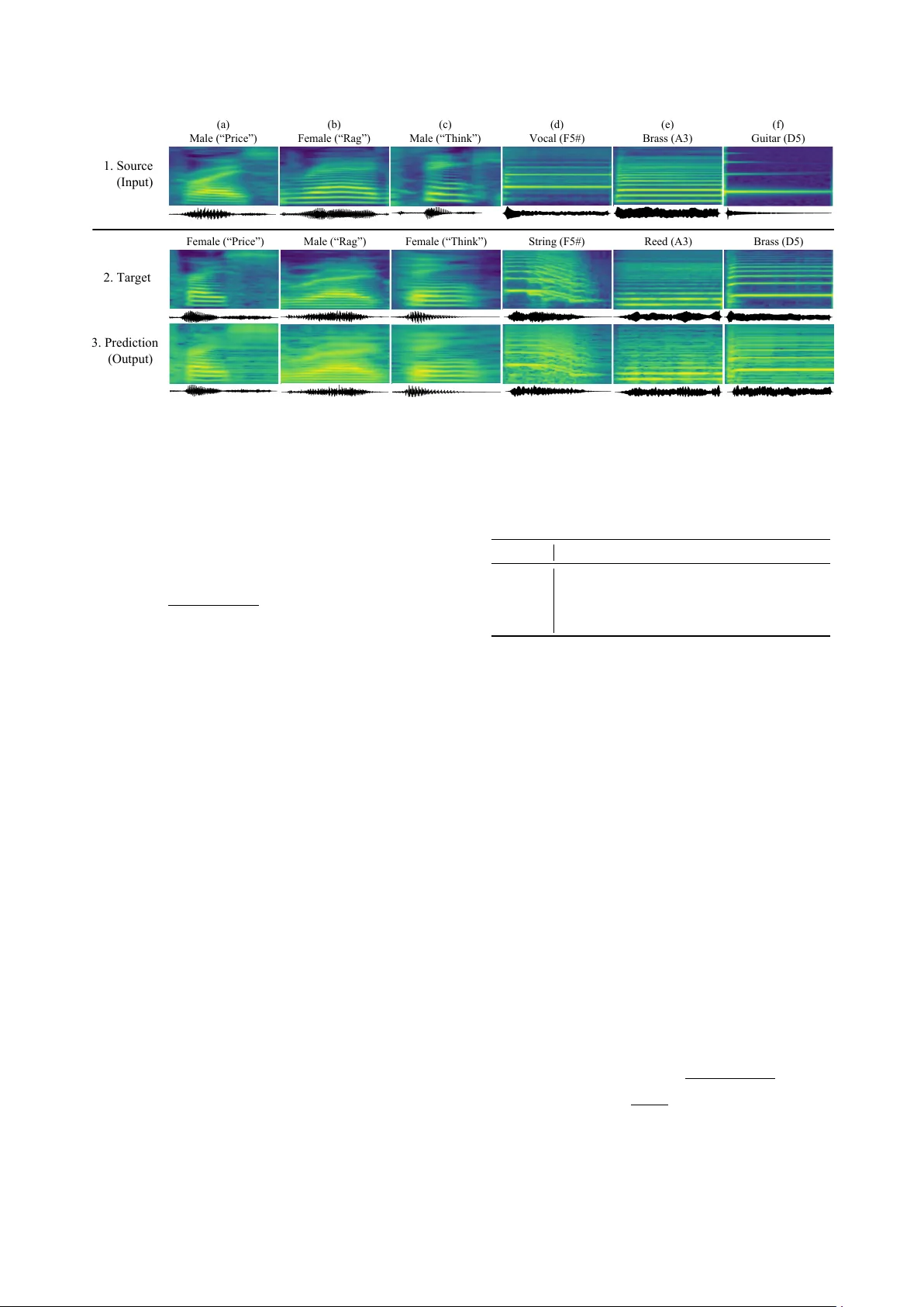
Conditional End-to-End A udio T ransf orms Albert Haque 1 ∗ , Michelle Guo 1 ∗ , Prateek V erma 2 1 Department of Computer Science 2 Center for Computer Research in Music and Acoustics Stanford Uni versity , USA Abstract W e present an end-to-end method for transforming audio from one style to another . For the case of speech, by conditioning on speaker identities, we can train a single model to transform words spoken by multiple people into multiple tar get voices. For the case of music, we can specify musical instruments and achiev e the same result. Architecturally , our method is a fully- differentiable sequence-to-sequence model based on con volu- tional and hierarchical recurrent neural networks. It is designed to capture long-term acoustic dependencies, requires minimal post-processing, and produces realistic audio transforms. Abla- tion studies confirm that our model can separate speak er and instrument properties from acoustic content at different con- text sizes. Empirically , our method achiev es competitiv e per- formance on community-standard datasets. 1. Introduction Humans are able to seamlessly process dif ferent audio repre- sentations despite syntactic, acoustic, and semantic variations. Inspired by humans, modern machine translation systems often use a word-le vel model to aid in the translation process [1, 2]. Many of these models are being used to model dependencies in music and speech for applications such as learning a latent space for representing speech, for text to speech and speech to text systems [3, 4]. In the case of text-based translation, learned word vectors or one-hot embeddings are the primary means of representing natural language [5, 6]. For speech and acoustic inputs ho wev er , word or phone embeddings are often used as a training con venience to provide multiple sources of informa- tion gradient flo w to the model [7, 8]. Spectrograms remain the dominant acoustic representation for both phoneme and word- lev el tasks since the high sampling rate and dimensionality of wa veforms is dif ficult to model [9]. In this paper , we address the task of end-to-end audio trans- formations, distinct from speech recognition (speech-to-text) and speech synthesis (text-to-speech). Specifically , we propose a fully-dif ferentiable audio transformation model. Given an au- dio input (e.g. spoken w ord, single music note) conditioned on the speaker or instrument, the model learns to predict a out- put spectrogram for any arbitrary target speaker or instrument. Our framew ork is generic and can be applied across multiple applications including timbre transfer , accent transfer, speaker morphing, audio effects, and emotion transformation. Current models often require complex pipelines consisting of domain-specific or fine-tuned features [10]. By contrast, our model does not require hand-crafted pipelines and only requires conditioning on input-output types. W e evaluate our model on two tasks: (i) transforming words spoken by a human into mul- tiple target voices, and (ii) playing a note on an instrument and transforming the note into another instrument’ s while retaining ∗ Equal contribution. the pitch. W e would like to make a key point: W e do not sup- ply the pitch variation, spectral or ener gy en velop to our model. Similarly for the output audio, parameters for synthesis are not provided b ut are instead learned from the desired mapping. Our method operates on spectrograms and takes inspira- tion from Listen-Attend-Spell [11] and T acoTron [4, 12], and is combined with ideas from natural language processing [13]. Our contributions are tw o fold: 1. W e present a fully differentiable end to end pipeline to per- form audio transformations by conditioning on specific in- puts and outputs for applications in speech and music. 2. W e demonstrate that our model’ s learned embeddings pro- duce a meaningful feature representation directly from speech. Our model transforms a spectrogram into a tar- get spectrogram, with the only supervision being the in- put speaker identity and the requested target speaker . Our method has the fle xibility to capture long term dependencies present in audio. 1.1. Related W ork V oice Con version. Our work is related to the problem of voice con version (VC) [14, 15]. Several works have approached VC using statistical methods based on Gaussian mixture mod- els, which typically inv olves using parallel data [16]. Other works have also used neural network-based frameworks using restricted Boltzmann machines or feed-forward neural networks [17]. While most VC approaches require parallel source and target speech data, collecting parallel data can be expensi ve. Thus, fe w works have proposed parallel-data-free frameworks [18]. In our proposed method, time-aligned source and target speech data is not a prerequisite. Recently , generative adversarial networks (GANs) hav e shown promise in image generatation and more recently in speech processing [19]. W e refer the reader to the voice con ver - sion challenge [20] for a more complete surv ey of VC methods. Style T ransfer . Our task of transforming audio from one style to another is closely related to the task of style transfer [21]. In visual style transfer [21, 22], the computed loss is typ- ically a linear combination of the style and content loss, ensur - ing that the output is semantically similar to the input, despite variations in color and texture. By contrast, our work directly computes the loss on the output and ground truth spectrograms. There have been works on similar lines for audio domain. In [23], V erma et al. provided an additional loss term, specific for audio, to transform musical instruments. Recent w ork on speech texture generation [24] shows promise of similar ideas and techniques for learning an end to end completely dif feren- tible pipeline. In [25], the authors introduced a version of vec- tor quantization using variational autoencoders, which learned a code for a particular speech utterance and were able to achie ve voice con version by passing on additional speaker cues. Devel- oped concurrently with our work, style tokens [26] and musical translation [27] show the capabilities of unsupervised learning in the audio domain. T ext-to-Speech. Also known as speech synthesis, text-to- speech (TTS) systems have just recently started to show promis- ing results. It has been sho wn that a pre-trained HMM com- bined with a sequence-to-sequence model can learn appropri- ate alignments [28]. Unfortunately this is not end-to-end as it predicts vocoder parameters and it is unclear ho w much perfor- mance is gained from the HMM aligner . Char2wa v [29] is an- other method, trained end-to-end on character inputs to produce audio but also predicts vocoder parameters. These models show promise of capturing semantic, speaker and word level informa- tion in an small latent space which can be used for conditioning the text in a sequence to sequence decoder . DeepV oice [30] improv es on this by replacing nearly all components in a stan- dard TTS pipeline with neural networks. While this is closer to- wards a fully differentiable solution, each component is trained in isolation with different optimization objectiv es. [24] showed a fully dif ferentiable end to end speech modification pipeline but the results were not con vincing in terms of audio quality and was more to sho w a proof of concept. W av eNet [9] is a powerful generativ e model of audio and generates realistic output speech. Howe ver it is slo w due to audio sample-lev el autoregressiv e nature and requires domain- specific linguistic feature engineering. Our work take cues from the work done for personalization of chatbot response which condition the output of sequence to sequence models [13] to achiev e consistent responses. W e deploy a similar strategy by conditioning on the type of audio transformation we need for the input audio. Also similar is T acotron line of work [4, 12]. In T acotron [4], the authors move even closer to a fully differen- tiable system. The input to T acotron [4] is a sequence of char- acter embeddings and the output is a linear-scale spectrogram. After applying Grif fin-Lim phase reconstruction [31], the wa ve- form is generated. 2. Method Our method is a sequence-to-sequence model [32] with atten- tion. The encoder consists of a con volutional and pyramidal recurrent network [33]. The decoder is a recurrent network. 2.1. Encoder Con volutional Network. Modeling the full spectrogram would require unrolling of the encoder RNN for an infeasibily large number of timesteps [34]. Even with truncated backpropaga- tion through time [35], this would be a challenging task on large datasets. Inspired by the Con volutional, Long Short-T erm Memory Deep Neural Network (CLDNN) [34] approach, we use a con volutional network to (i) reduce the temporal length of the input by using a learned con volutional filter bank. The stride, or hop size, controls the degree of length reduction. (ii) CNNs are good feature extractor that help the temporal unit bet- ter in modelling the longer dynamical features. Pyramidal Recurrent Network. Inspired by the Clock- work RNN [33], we use a pyramidal RNN to address the issue of learning from a lar ge number of timesteps [11]. A pyramidal RNN is the same as a standard multi-layer RNN but instead of each layer simply accepting the input from the previous layer , successiv ely higher layers in the network only compute, or “tick, ” during particular timesteps. This allows different layers of the RNN to operate at different temporal scales. W av eNet [9] Input Spectrogram Latent Code Source Conditioning CNN Target Conditioning Output Spectrogram (Transformed) Figure 1: Overview of our model. Y ellow and green boxes de- note one-hot vectors used to condition the input to each RNN. Solid lines indicate data flow . Dashed lines indicate temporal state sharing. Gray r ectangles denote learned r epr esentations. also controls the temporal receptiv e field at each layer of their network with dilated con volutions [36, 37]. Formally , let h j i de- note the hidden state of a long short-term memory (LSTM) cell at the i -th timestep of the j -th layer: h j i = LSTM ( h j i − 1 , h j − 1 i ) For a pyramidal LSTM (pLSTM ), the outputs from the immedi- ately preceding layer , which contains high-resolution temporal information, are concatenated: h j i = pLSTM  h j i − 1 , h h j − 1 2 i , h j − 1 2 i +1 i . (1) In (1), the output of a pLSTM unit is now a function of not only its previous hidden state, but also the outputs from two timesteps from the layer below . Not only does the pyramidal RNN provide higher-le vel temporal features, b ut it also reduces the inference comple xity . Only the first layer processes each input timestep as opposed to all layers. The input time slice into the encoder is conditioned on the speaker ID. This is done by concatenating a one-hot speak er encoding with the CNN output at each time step, before being fed into the recurrent network. 2.2. Decoder Attention . Learning long-range temporal dependencies can be challenging [38]. T o aid this process, we use an attention-based LSTM transducer [39, 40]. At each timestep, the transducer produces a probability distribution o ver the next spectrogram time-slice conditioned on all pre viously seen inputs. The dis- tribution for y i is a function of decoder state s i and context c i . (b) Female (“Rag”) Male (“Rag”) (d) Vocal (F5#) String (F5#) (a) Male (“Price”) Female (“Price”) (e) Brass (A3) Reed (A3) Brass (D5) (f) Guitar (D5) (c) Male (“Think”) Female (“Think”) 1. Source (Input) 2. Target 3. Prediction (Output) Figure 2: Spectrogram results. Examples on TIMIT (2a-c) and NSynth (2d-f). The speakers and instruments wer e pr esent in the training set b ut the test set contained unseen vocabulary wor ds or notes. The x axis denotes time and the y axis denotes fr equency . The input, gr ound truth tar get, and our model’ s pr ediction ar e shown. The corresponding waveform is shown beneath eac h spectr ogr am. The decoder state s i is a function of previous state s i 1 , previ- ously emitted time-slice y i 1 , context c i 1 and one hot encoding of the desired output transformation similar to [13]. The context vector c i is produced by an attention mecha- nism [11]. Specifically , we define: α i,j = exp( e i,j ) P L j =1 exp( e i,j ) and c i = X u α i,u h u (2) where attention α i,j is defined as the alignment between the current decoder time-slice i and a time-slice j from the encoder input. The score between the output of the encoder (i.e., hid- den states), h j , and the previous state of the decoder cell, s i − 1 is computed with: e i,u = h φ ( s i ) , ϕ ( h u ) i where φ and ϕ are multi-layer perceptrons: e i,j = w T tanh( W s i − 1 + V h j + b ) with learnable parameters w , W and V . 3. Experiments Datasets. W e evaluate our model on two audio transforma- tion tasks: (i) voice con version and (ii) musical style transfer . The TIMIT [41] and NSynth [42] datasets were used (T able 1). Speech examples from AudioSet [43] were used to pre-train the model as an autoencoder . W e condition our model on the source and target style. For the case of speech, style refers to the speaker . For NSynth, it refers to the instrument type. For all experiments, we focus on transformations on a word- or pitch-lev el. This was primarily for demonstration – adding sentence level transformations would have limited the number of training examples. Howe ver , we note that sequence- to-sequence models are capable of encoding sentence lev el in- formation in a small latent encoding vector [11]. Similarly , the decoder can model full sentences, as shown in T acotron [4]. A udio Format. All experiments used a sampling rate of 16 kHz with pre-emphasis of 0.97. Audio spectrograms were com- puted with Hann windowing, 50 ms window size, 12.5 ms hop size, and a 2048-point Fourier transform. Mel-spectrograms were visualized using an 80 channel mel-filterbank. Optimization. The model was optimized with Adam [44] with β 1 = 0 . 9 , β 2 = 0 . 999 and  = 10 − 8 . The mean squared error was used as the loss objectiv e. A learning rate of 10 − 3 was T able 1: Overview of datasets. W e evaluate our method on voice con version and musical style transfer . TIMIT [41] NSynth [42] AudioSet [43] Styles 630 speakers 1,006 types 7 classes Content 6,102 words 88 pitches — T rain 39,834 289,205 1,010,480 T est 14,553 4,096 — used with an exponential decay factor of 0.99 after e very epoch. The batch size for all datasets was 128. Models were trained for 20 epochs on NSynth and 50 epochs on TIMIT . T o train the decoder , we apply the standard maximum-likelihood training procedure, also known as teacher-forcing [45], which has been shown to improv e con ver gence. The model was implemented and trained with T ensorflow on a single Nvidia V100 GPU. Baselines. W e e valuate three methods for audio transfor- mations. First, we ev aluate the classical sequence-to-sequence (Seq2Seq) model [32] which consists of a vanilla RNN as the encoder and a different RNN as the decoder . Second, we ev al- uate Listen, Atten, and Spell (LAS) [11]. This is the same as the seq2seq model but the decoder is equipped with an atten- tion mechanism that allows it to “peek” at the encoder outputs. Additionally they use a pyramidal RNN. Third, we ev aluate a conditional sequence-to-sequence model (C-Seq2Seq). This is the same as Seq2Seq but with our conditioning mechanism. Evaluation Metrics. W e use subjective and objecti ve met- rics for both voice con version and musical style transfer: • Mean opinion score (MOS), higher is better . • Mel-cepstral distortion (MCD), lower is better . • Side-by-side rating, higher is better . Mel-Cepstral Distortion. Let y and ˆ y denote the ground truth and predicted mel-spectorgram, respecti vely . The MCD is: MCD ( y , ˆ y ) = 10 ln(10) v u u t 2 T X t =1 || y t − ˆ y t || (3) where T is the number of timesteps and t is the timestep slice. T able 2: Comparison to existing methods. W e measure mean opinion scor e (MOS) and mel-cepstral distortion (MCD) on voice con version and musical style tr ansfer . Higher MOS is better . Lower MCD is better . The 95% confidence interval for TIMIT MOS and MCD values ar e ± 0 . 024 and ± 0 . 017 , r espec- tively , and for NSynth, ± 0 . 016 and ± 0 . 053 . C-Seq2Seq is a vanilla conditioned seq-to sequence model. MOS MCD Method TIMIT NSynth TIMIT NSynth Ground T ruth 4.65 4.16 — — Seq2Seq [32] 3.37 3.13 7.31 11.18 LAS [11] 3.52 3.23 7.40 11.24 C-Seq2Seq 3.50 3.36 7.26 10.81 Our Method 3.88 3.43 6.49 10.35 3.1. Results W e present results on no vel v ocabulary w ords and pitches. Fig- ure 2 shows results on the test set, which contain words and pitches not present in the training set. Our model is able to capture fundamental phonetic properties of each speaker or in- strument and apply these properties to nov el words and pitches. 3.1.1. Mean Opinion Score T o evaluate generativ e models, subjecti ve scores [12] or percep- tual metrics [22] are often used. W e follow this same procedure for audio generated by our model by randomly selecting a fixed set of 50 test set examples. Audio generated from all baseline models on this set were rated by at least three normal-hearing human raters. A total of 10 raters participated in the study and listened to the generated audio with the same over -ear head- phones. The rating scale is a 5-point numeric scale: 1. bad, 2. poor , 3. fair , 4. good, and 5. excellent. Higher v alues are better . The results of this study are shown in T able 2. Also shown in T able 2 are the mel-cepstral distances. 3.1.2. Side-by-Side Evaluation W e also conducted a side-by-side ev aluation between audio generated by our system and the ground truth. For each prediction-ground truth audio pair , we asked raters to gi ve a score ranging from -1 (generated audio is worse than ground truth) to +1 (generated audio is better than ground truth). The mean score was − 0 . 74 ± 0 . 22 , where 0.22 denotes the 95% confidence interval. This indicates that raters have a preference tow ards the ground truth. 3.1.3. Learned Style Representations Figure 3 shows the learned representations for the musical trans- formation task. Our model can successfully cluster sounds belonging to pitch classes, rather than individual frequencies. More interestingly , from an acoustic signals perspective, a mu- sical octave is denoted by plus/minus 12, where 12 is the stan- dard MIDI pitch number . MIDI pitch 74 is one octave above MIDI 62. The resulting pitch 74 is double the frequency of pitch 62. Howe ver , pitch 74 is closer to 62 than 67, despite 67 being closer to 64 in absolute pitch. This is because 62 and 74 hav e high amounts of harmonic overlap. For audio transforms, this confirms our model can learn acoustic attributes without explicit supervision. Figure 3: Learned representations. Each dot denotes an audio clip. Colors denote pitches. The x and y axes are T -SNE [46] pr ojections. Colored text denotes the musical pitch (e.g., D#2 r efers to the note D#, 2nd octave). Dashed cir cles indicate pitc h classes. Despite not given any explicit pitch labels, the model was able to cluster similar musical notes. 3.1.4. Acoustic Context Size Music demonstrates dif ferent acoustic properties compared to speech [47]. For example, speech often contains more variances in pitch whereas musical notes are held constant on the order of tens to hundreds of milliseconds. The acoustic context size denotes t he conte xtual windo w modeled by each hidden state of our network. Larger conte xts capture more acoustic content. As shown in T able 3, the context size does not significantly alter the mel-cepstral distance. All MCD values are between 10.3 and 10.7. Compare this to speech on TIMIT : a context size of 50 ms captures enough temporal context without ov erwhelming (i.e., smoothing) the hidden state. Larger fields of size 100-200 ms produce lower quality transforms. T able 3: Acoustic context size. W e varied the per timestep context size and measured MCD. Lower values ar e better . Plus/minus values denote the 95% confidence interval. Context Size TIMIT NSynth 12.5 ms 7 . 28 ± 0 . 02 10 . 35 ± 0 . 05 25 ms 7 . 03 ± 0 . 02 10 . 47 ± 0 . 04 50 ms 6 . 49 ± 0 . 01 10 . 48 ± 0 . 05 100 ms 7 . 11 ± 0 . 02 10 . 69 ± 0 . 04 200 ms 7 . 32 ± 0 . 02 10 . 67 ± 0 . 05 4. Conclusion In this work, we presented an end-to-end method for transform- ing audio from one style to another . Our method is a sequence- to-sequence model consisting of con volutional and recurrent neural networks. By conditioning on the speaker or instrument, our method is able to transform audio for unseen words and mu- sical notes. Subjectiv e tests confirm the quality of our model’ s generated audio. Overall, this work alle viates the need for com- plex audio processing pipelines and sheds new insights on the capabilities of end-to-end audio transformations. W e hope oth- ers will build on this work and extend the capabilities of end-to- end audio transforms. Acknowledgements. W e would like to thank Malcolm Slaney and Dan Jurafsky for helpful feedback. Additionally , we thank members of the Stanford AI Lab for participating in subjectiv e experiments. 5. References [1] M.-T . Luong, H. Pham, and C. D. Manning, “Ef fectiv e approaches to attention-based neural machine translation, ” arXiv , 2015. [2] W . Y . Zou, R. Socher, D. M. Cer , and C. D. Manning, “Bilin- gual word embeddings for phrase-based machine translation. ” in EMNLP , 2013. [3] C.-C. Chiu, T . N. Sainath, Y . Wu, R. Prabhav alkar , P . Nguyen, Z. Chen, A. Kannan, R. J. W eiss, K. Rao, K. Gonina et al. , “State- of-the-art speech recognition with sequence-to-sequence models, ” arXiv , 2017. [4] Y . W ang, R. Skerry-Ryan, D. Stanton, Y . W u, R. J. W eiss, N. Jaitly , Z. Y ang, Y . Xiao, Z. Chen, S. Bengio et al. , “T acotron: T owards end-to-end speech synthesis, ” arXiv , 2017. [5] J. Pennington, R. Socher, and C. D. Manning, “Glove: Global vectors for word representation. ” in EMNLP , 2014. [6] T . Mikolov , K. Chen, G. Corrado, and J. Dean, “Efficient estima- tion of word representations in vector space, ” arXiv , 2013. [7] H. Bourlard and N. Morgan, “ A continuous speech recognition system embedding mlp into hmm, ” in NIPS , 1990. [8] J. G. W ilpon, L. R. Rabiner, C.-H. Lee, and E. Goldman, “ Au- tomatic recognition of keywords in unconstrained speech using hidden markov models, ” ICASSP , 1990. [9] A. v . d. Oord, S. Dieleman, H. Zen, K. Simonyan, O. V inyals, A. Grav es, N. Kalchbrenner , A. Senior , and K. Ka vukcuoglu, “W avenet: A generati ve model for raw audio, ” arXiv , 2016. [10] A. Kain and M. W . Macon, “Spectral voice con version for text-to- speech synthesis, ” in ICASSP . IEEE, 1998. [11] W . Chan, N. Jaitly , Q. Le, and O. V inyals, “Listen, attend and spell: A neural network for large vocabulary conv ersational speech recognition, ” in ICASSP , 2016. [12] J. Shen, R. Pang, R. J. W eiss, M. Schuster , N. Jaitly, Z. Y ang, Z. Chen, Y . Zhang, Y . W ang, R. Skerry-Ryan, R. A. Saurous, Y . Agiomyrgiannakis, and Y . W u, “Natural tts synthesis by condi- tioning wavenet on mel spectrogram predictions, ” in Interspeech , 2018. [13] J. Li, M. Galley , C. Brockett, G. P . Spithourakis, J. Gao, and B. Dolan, “ A persona-based neural conversation model, ” arXiv , 2016. [14] M. Abe, S. Nakamura, K. Shikano, and H. Kuw abara, “V oice con- version through vector quantization, ” Journal of the Acoustical Society of J apan , 1990. [15] Y . Stylianou, O. Capp ´ e, and E. Moulines, “Continuous probabilis- tic transform for voice con version, ” T rans. on speech and audio pr ocessing , 1998. [16] T . T oda, A. W . Black, and K. T okuda, “V oice con version based on maximum-likelihood estimation of spectral parameter trajectory , ” T ASLP , 2007. [17] S. H. Mohammadi and A. Kain, “V oice conversion using deep neural networks with speaker-independent pre-training, ” in Spo- ken Language T echnology W orkshop , 2014. [18] T . Kinnunen, L. Juvela, P . Alku, and J. Y amagishi, “Non-parallel voice con version using i-vector plda: T ow ards unifying speaker verification and transformation, ” in ICASSP , 2017. [19] T . Kaneko, H. Kameoka, K. Hiramatsu, and K. Kashino, “Sequence-to-sequence voice con version with similarity metric learned using generativ e adversarial networks, ” in Interspeech , 2017. [20] T . T oda, L.-H. Chen, D. Saito, F . V illavicencio, M. W ester , Z. Wu, and J. Y amagishi, “The voice conv ersion challenge 2016. ” in In- terspeech , 2016. [21] L. Gatys, A. S. Ecker , and M. Bethge, “T exture synthesis using con volutional neural networks, ” in NIPS , 2015. [22] J. Johnson, A. Alahi, and L. Fei-Fei, “Perceptual losses for real- time style transfer and super-resolution, ” in ECCV , 2016. [23] P . V erma and J. O. Smith, “Neural style transfer for audio spec- tograms, ” arXiv , 2018. [24] J. Chorowski, R. J. W eiss, R. A. Saurous, and S. Bengio, “On us- ing backpropagation for speech texture generation and voice con- version, ” arXiv , 2017. [25] A. van den Oord, O. V inyals et al. , “Neural discrete representation learning, ” in NIPS , 2017. [26] Y . W ang, D. Stanton, Y . Zhang, R. Skerry-Ryan, E. Battenberg, J. Shor, Y . Xiao, F . Ren, Y . Jia, and R. A. Saurous, “Style tokens: Unsupervised style modeling, control and transfer in end-to-end speech synthesis, ” arXiv , 2018. [27] N. Mor , L. W olf, A. Polyak, and Y . T aigman, “ A universal music translation network, ” arXiv , 2018. [28] W . W ang, S. Xu, and B. Xu, “First step tow ards end-to-end para- metric tts synthesis: Generating spectral parameters with neural attention, ” in Interspeech , 2016. [29] J. Sotelo, S. Mehri, K. Kumar, J. F . Santos, K. Kastner , A. Courville, and Y . Bengio, “Char2wav: End-to-end speech syn- thesis, ” arXiv , 2017. [30] S. O. Arik, M. Chrzano wski, A. Coates, G. Diamos, A. Gibiansky , Y . Kang, X. Li, J. Miller, J. Raiman, S. Sengupta et al. , “Deep voice: Real-time neural text-to-speech, ” arXiv , 2017. [31] S. Nawab, T . Quatieri, and J. Lim, “Signal reconstruction from short-time fourier transform magnitude, ” TASLP , 1983. [32] I. Sutske ver , O. V inyals, and Q. V . Le, “Sequence to sequence learning with neural networks, ” in NIPS , 2014. [33] J. K outnik, K. Greff, F . Gomez, and J. Schmidhuber, “ A clock- work rnn, ” arXiv , 2014. [34] T . N. Sainath, R. J. W eiss, A. Senior , K. W . Wilson, and O. V inyals, “Learning the speech front-end with raw wav eform cldnns, ” in Interspeech , 2015. [35] S. S. Haykin et al. , Kalman F iltering and Neural Networks . Wi- ley Online Library , 2001. [36] P . Dutilleux, “ An implementation of the algorithme ` a trous to compute the wav elet transform, ” in W avelets . Springer, 1990. [37] F . Y u and V . Koltun, “Multi-scale context aggregation by dilated con volutions, ” arXiv , 2015. [38] Y . Bengio, P . Simard, and P . Frasconi, “Learning long-term de- pendencies with gradient descent is difficult, ” T rans. on Neural Networks , 1994. [39] J. K. Chorowski, D. Bahdanau, D. Serdyuk, K. Cho, and Y . Ben- gio, “ Attention-based models for speech recognition, ” in NIPS , 2015. [40] D. Bahdanau, K. Cho, and Y . Bengio, “Neural machine translation by jointly learning to align and translate, ” arXiv , 2014. [41] J. S. Garofolo, L. F . Lamel, W . M. Fisher, J. G. Fiscus, and D. S. Pallett, “Darpa timit acoustic-phonetic continous speech corpus cd-rom. nist speech disc 1-1.1, ” NASA STI , 1993. [42] J. Engel, C. Resnick, A. Roberts, S. Dieleman, D. Eck, K. Si- monyan, and M. Norouzi, “Neural audio synthesis of musical notes with wav enet autoencoders, ” 2017. [43] J. F . Gemmeke, D. P . W . Ellis, D. Freedman, A. Jansen, W . Lawrence, R. C. Moore, M. Plakal, and M. Ritter , “ Audio set: An ontology and human-labeled dataset for audio events, ” in ICASSP , 2017. [44] D. P . Kingma and J. Ba, “ Adam: A method for stochastic opti- mization, ” ICLR , 2015. [45] R. J. W illiams and D. Zipser, “ A learning algorithm for contin- ually running fully recurrent neural networks, ” Neural computa- tion , 1989. [46] L. v . d. Maaten and G. Hinton, “V isualizing data using t-sne, ” JMLR , 2008. [47] B. Gold, N. Morgan, and D. Ellis, Speech and audio signal pro- cessing: processing and per ception of speech and music . John W iley & Sons, 2011.