Learning a Latent Space of Multitrack Measures
Discovering and exploring the underlying structure of multi-instrumental music using learning-based approaches remains an open problem. We extend the recent MusicVAE model to represent multitrack polyphonic measures as vectors in a latent space. Our …
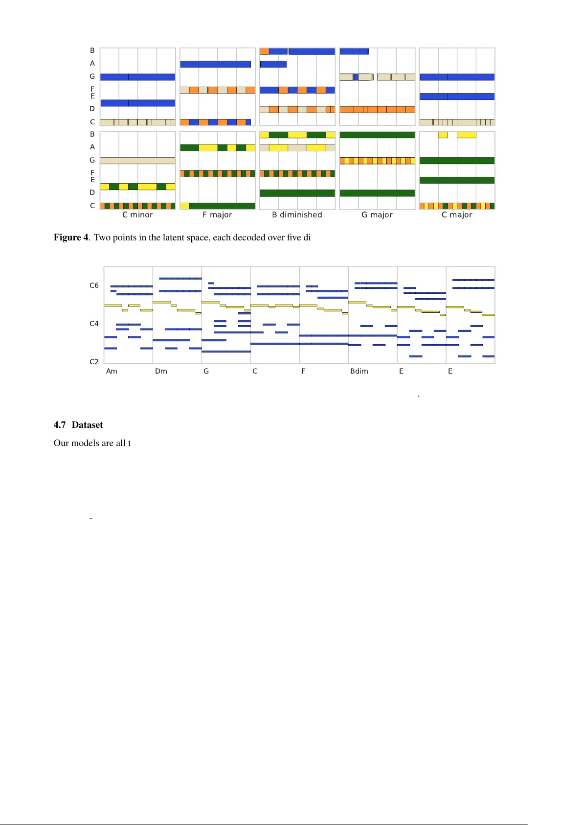
Authors: Ian Simon, Adam Roberts, Colin Raffel
LEARNING A LA TENT SP A CE OF MUL TITRA CK MEASURES Ian Simon Adam Roberts Colin Raffel Jesse Engel Curtis Hawthorne Douglas Eck Google Brain { iansimon,adarob,craffel,jesseengel,fjord,deck } @google.com ABSTRA CT Discov ering and exploring the underlying structure of multi-instrumental music using learning-based approaches remains an open problem. W e extend the recent MusicV AE model [33] to represent multitrack polyphonic measures as vectors in a latent space. Our approach enables sev- eral useful operations such as generating plausible mea- sures from scratch, interpolating between measures in a musically meaningful way , and manipulating specific mu- sical attributes. W e also introduce chord conditioning, which allo ws all of these operations to be performed while keeping harmony fixed, and allo ws chords to be changed while maintaining musical “style”. By generating a se- quence of measures ov er a predefined chord progression, our model can produce music with con vincing long-term structure. W e demonstrate that our latent space model makes it possible to intuitively control and generate mu- sical sequences with rich instrumentation (see https: //goo.gl/s2N7dV for generated audio). 1. INTR ODUCTION Recent advances in machine learning have made it possible to train generativ e models which can accurately represent and generate many different types of objects such as im- ages, sketches [15], and piano performances [37], to name a few . Some of these models learn a latent space : a lower- dimensional representation that can be mapped to and from the object space. A major advantage of such latent space models is that many operations that would be difficult to perform in the object space, like morphing between two objects in a semantically meaningful way , become straight- forward arithmetic in the latent space. It has ev en been claimed that latent space models can augment human un- derstanding of the object domain [6]. Latent space models hav e already been trained for several musical concepts in- cluding raw wa v eforms of notes [12], melodies and drum tracks [33], and playlists [38]. Such models are also fre- quently used for music recommendations [23], where both user “taste” and song “style” are reasoned about in terms of latent vectors. In this paper , we present a latent space model of indi vid- ual measures of music with multi-instrument polyphony and dynamics. One way to think about such objects is as musical textur es ; howe ver , we do not model the audio it- self b ut rather use a symbolic representation of the music. This latent space model allows us to perform a number of intuitiv e operations: • Sample a measure from the prior distribution to gen- erate nov el music from scratch. • Interpolate (i.e. slowly morph) between two mea- sures in a semantically meaningful way . • Apply attribute transformations to an existing mea- sure, e.g. “increase note density” or “add strings”. The latent space model can also be augmented with addi- tional conditioning variables, which we demonstrate with chords. Chord conditioning allo ws us to perform the abo ve operations while holding chords constant or to change chords while keeping musical texture constant. Even though this model only represents indi vidual mea- sures and thus is incapable of generating long-term struc- ture on its own, combining the latent space with chord conditioning makes it fairly easy to generate music with con vincing long-term dependencies; e.g. a composer could pick a single point in the latent space and then decode that point (or slo wly interpolate between two points) o ver a de- sired chord progression. The contrib utions of this paper are as follows: 1. An e xtension of the MusicV AE model [33] to handle up to 8 tracks played by arbitrary MIDI programs. 2. A nov el ev ent-based track representation that han- dles polyphony , micro-timing, dynamics, and instru- ment selection. 3. Introducing chord-conditioning to a latent space model, so that chords and arrangement/orchestration can be controlled independently . 2. RELA TED WORK Our work builds on a long history of past efforts at sym- bolic music generation, plus more recent interest in la- tent spaces and modeling interplay between instruments. Algorithmic music generation has been a topic of inter- est for at least 200 years [22, 27, 34]. Prior to the recent neural network renaissance, most systems, such as that of Cope [9], used human-encoded rules, Markov models, or a few other method categories as described by Fern ´ andez and V ico [13] and Papadopoulos and W iggins [29] in re- cent surve ys. The use of neural networks in symbolic music genera- tion has seen a resur gence in interest, as surv eyed by Briot et al. [4]. Early work on neural networks for symbolic music generation includes Bharucha and T odd [1], Mozer [28], Chen and Miikkulainen [7], and Eck and Schmid- huber [11]. One of the first effecti ve neural network sys- tems for generating polyphonic music is from Boulanger - Lew ando wski et al. [3], who use a recurrent model o ver a pianoroll representation to generate classical and folk music. The pianoroll is a fairly standard representation for polyphonic music generation; we instead use an e vent- based representation closer to the MIDI standard itself. Some work in music generation has been focused on specific domains. One such popular domain for poly- phonic music generation is Bach chorales: DeepBach [16], CoCoNet [18], and BachBot [24] are all different gener- ativ e models for polyphonic Bach chorales that can re- spond to user input. In contrast, our model presented in this paper works simultaneously across multiple W estern music styles including classical, jazz, and pop/rock; essen- tially any music e xpressible with MIDI notes and program changes is compatible. Because of its latent space rep- resentation, our model is also able to interpolate between these different domains. Other recent systems for generating polyphonic music include JamBot [5] which generates chords then notes in a two-step process, DeepJ [25] which generates polyphonic piano music where a user can control se veral style param- eters, a model from Roy et al. [35] that generates varia- tions on lead sheets, and Song from PI [8] which generates melody , chord, and drum tracks using a hierarchical recur - rent network combined with hand-engineered features. There are also commercial software systems such as PG Music’ s Band-in-a-Box [14] and T echnimo’ s iReal Pro [2] that generate multi-instrumental music over user-specified chord progressions. Howe v er , these products appear to support a limited and fixed number of preset arrangement styles combined with rule-based modifications. Perhaps the most similar systems to our current work are MusicV AE from Roberts et al. [33] (which we directly extend) and MuseGAN from Dong et al. [10] (which builds upon the work of Y ang et al. [42]). MuseGAN [10] is based on generativ e adversarial networks (GANs) and is capable of modeling multiple instruments over multiple bars. Like our work, the system uses a latent space shared across tracks to handle interdependencies between instru- ments. Howe v er , in MuseGAN the set of instruments is a fixed quintet consisting of bass, drums, guitar , piano, and strings, whereas our system handles arbitrary instru- ment combinations. Separately , MuseGAN is focused on accompaniment and generation and is unable to represent or manipulate preexisting music. Our system can also gen- erate from scratch, but in contrast with MuseGAN, it can also facilitate user-dri ven manipulation of existing music via the latent space. The MusicV AE architecture introduced by Roberts et al. [33] is able to learn a latent space of musical sequences using a novel hierarchical decoder that allo ws it to model long-term structure and multi-instrument sequences. Ho w- ev er , this w ork applies strict constraints to the sequences to reach its goals. In order to guarantee a constant number of ev ents per measure, non-drum tracks are limited to mono- piano C3 C4 C5 bass C2 C3 saxophone C4 C5 C6 drums C2 C3 C4 Figure 1 . A single measure consisting of 4 tracks, shown as separate pianorolls. Each track is represented as a MIDI- like sequence of note-on , note-off , time-shift , and velocity- change ev ents, with a single pr o gram-select event at the beginning and an end-tr ack event at the end. For all other figures in this paper, multiple tracks are combined into a single pianoroll, color-coded by instrument f amily . phonic sequences, and all tracks are represented with a sin- gle velocity and quantized at the le v el of 16 th notes. This reduces the challenge of modeling longer-term structure, but at the expense of expressi veness. Furthermore, while the “trio” MusicV AE is capable of modeling three broad instrument classes–melody , bass, and drums–it is limited to exactly three instruments, arbitrarily excluding poten- tially pivotal voices and disregarding the specific identity of each instrument (e.g. eletric guitar and piano are both considered “melody” instruments). Further, Roberts et al. do not consider modeling fine-grai ned timing and velocity , nor do the y develop a method for chord conditioning. Ne v- ertheless, the MusicV AE architecture and its implementa- tion provide a powerful basis for exploring a more expres- siv e and complete multitrack latent space, and thus we po- sition our work as an extension of it. 3. MEASURE REPRESENT A TION W e model measures with up to 8 tracks (see Figure 1 for an e xample with 4 tracks). Each track consists of a single “instrument” as extracted by pretty midi [31]. A track is represented as a MIDI-like sequence of events from an extension of the vocabulary used by Simon and Oore [37] to handle metric timing and choice of instrument: • 128 note-on events, one for each MIDI pitch. • 128 note-off events, one for each MIDI pitch. • 8 velocity-change ev ents, MIDI velocity quantized into 8 bins. These e vents set the v elocity for subse- quent note-on ev ents. • 96 time-shift ev ents that shift the current time for- ward by the corresponding number of quantized time steps, where 24 steps is the length of a quarter note. • 129 program-select ev ents (128 programs plus drums) that set the MIDI program number at the be- ginning of each track. • A single end-track event, used to mark the end of each track. F or measures with fe wer than 8 tracks, missing tracks consist solely of the end-track ev ent. For simplicity we only include measures with exactly 96 quantized time steps (4 quarter notes), as this is the most frequent measure size in our dataset. 4. MODEL Our model is a v ariational autoencoder (V AE) [21] ov er hierarchical sequences, extending the architecture of MusicV AE [33] to handle variable numbers of tracks and ev ents per track. The top lev el of the decoder hierarchy produces track embeddings from a single latent code and the bottom lev el produces the sequence for each track, in- cluding the choice of instrument as a MIDI program num- ber . The encoder (which is also hierarchical) works in re- verse, first con verting each track to a single vector then mapping this sequence of track vectors to the latent space. W e achie v e additional control over the output of the model by adding chord conditioning to both the encoder and de- coder (see Section 4.4 for details). In the following sub- sections, we provide a brief ov ervie w of our model; for a more in-depth description of our baseline, see [33]. 4.1 V ariational A utoencoders An autoencoder is a model that learns to “compress” or en- code objects to a lower -dimensional latent space and then decode these latent representations back into the original objects. Autoencoders are typically trained to optimize a r econstruction loss which measures how close the recon- structed version is to the original object. This encourages the model to produce a compressed representation that cap- tures the important variation among the objects. The variational autoencoder extends the basic autoen- coder in that it considers the latent representation z to be a random variable drawn from a prior distribution p ( z ) , usu- ally a multiv ariate Gaussian with diagonal cov ariance. The encoder approximates the posterior distribution p ( z | x ) , while the decoder models the likelihood p ( x | z ) . The V AE is thus a generative model with the follo wing gen- eration process: generate a latent vector z from the prior distribution by sampling z ∼ p ( z ) , then use the decoder to sample an output using the sampled z by x ∼ p ( x | z ) . In a variational autoencoder , the encoder and decoder are typically neural networks q λ ( z | x ) and p θ ( x | z ) pa- rameterized by θ and λ , respecti v ely . In our case where we are dealing with sequences, both the encoder and decoder are hierarchical LSTM [17] models as in MusicV AE. This architecture has two ke y benefits: First, it is a la- tent variable model ; we can sample new measures and we can map existing measures to the latent space and trans- form them in various ways. Second, it is hier ar c hical ; in- dividual tracks are independent conditional on their em- beddings. The use of track embeddings gi v es the model a way to represent complex dependencies between tracks, so that tracks will “fit together” when generated. 4.2 Loss Function The V AE model optimizes a loss function that is the dif- ference of two terms: the reconstruction loss, and the Kullback-Leibler (KL) di ver gence loss: E [log p θ ( x | z )] − D KL ( q λ ( z | x ) k p ( z )) (1) The reconstruction loss term E [log p θ ( x | z )] maximizes the log-likelihood of the training data. In our model, the reconstruction loss is computed as the sum of the cross entropy between the predicted output distribution and the ground truth value over all ev ents on all tracks in a given sequence. The KL diver gence loss term D KL ( q λ ( z | x ) k p ( z )) encourages q λ ( z | x ) (the distri- bution produced by the encoder) to be close to p ( z ) , the unit Gaussian prior . One implication of optimizing a combination of loss terms is that there’ s a core tradeoff between two desires: 1. reconstruction : The model should be able to faith- fully represent measures from the training set in the latent space, such that these measures can be repro- duced from their latent code. 2. sampling : The prior should be enforced; i.e. the pos- terior distributions for encoded measures from the training set should be close to the prior . This ensures that measures sampled from the prior are plausible. W e control this tradeof f by using the “free bits” method of Kingma et al. [20]; the KL loss term is allo wed a bud- get τ bits of entropy per training example before it be- gins accruing loss. Increasing τ therefore improves recon- struction fidelity with the drawback of less realistic sam- ples and semantically meaningless interpolation. W e found τ = 64 produced a good trade-off between reconstruction and sampling/interpolation in most cases. The only ex- ception was in the attribute vector experiments described in Section 5.3, for which we found better results by using τ = 256 . Perhaps surprisingly , providing chords (see Sec- tion 4.4) had little ef fect on reconstruction accuracy (for a giv en τ ) even though samples from the chord-conditioned model do respect the chord conditioning. 4.3 Architectur e In this section, we give a brief overvie w of our model’ s architecture; for specific details refer to [33] and our pub- lic source code 1 . Our encoder consists of two le vels of bidirectional LSTMs. The first level independently con- sumes each of the 8 track e vent streams, concatenating the final outputs from the forward and backward directions to produce 8 track embeddings. The second level consumes these 8 embeddings, outputting a single embedding that is the concatenation of final states of the forward and back- ward directions. This embedding is then fed through two 1 https://github.com/tensorflow/magenta 1 2 3 4 5 6 7 8 C1 C3 C5 Figure 2 . An interpolation between two measures generated by our model. original C1 C3 C5 reconstructed increase range strings only more tracks Figure 3 . Multiple transformations to a single measure via attrib ute vector arithmetic. On the left is the original measure, followed by its reconstruction from the latent space. After that are three transformations: increasing the pitch range, using only string instruments, and using more tracks. fully-connected layers to produce the µ and, after a soft- plus activ ation, the σ parameter for the autoencoder’ s la- tent distribution. A latent vector is then sampled from a multiv ariate Gaussian distrib ution with a diagonal covari- ance, parameterized by µ and σ . The decoder is made up of two le vels of unidirectional LSTMs. The first level (called the “conductor” by Roberts et al.) is initialized by setting its state to be the result of passing the latent vector though a linear layer with a tanh activ ation. This conductor LSTM is then run for 8 steps with a null input, outputting 8 track embeddings. For each of the 8 tracks, the lo wer-le v el LSTM is initialized in the same manner as the conductor using one of the 8 track em- beddings. The initial input to the LSTM for each track is a zero v ector concatenated with the track embedding, and subsequent inputs are the one-hot representation of the pre- vious ev ent concatenated with the track embedding. The outputs of the LSTM are then passed through a final soft- max layer ov er the ev ent v ocabulary . 4.4 Conditioning While the latent space allows for the manipulation of in- dividual attributes, it is sometimes dif ficult to avoid intro- ducing side effects on correlated attributes. By condition- ing both the encoder and decoder on chords, we encourage the model to “factor out” chord information from the latent representation. This allo ws us to control chords and other attributes independently , which supports both holding the “arrangement” of the sequence constant while changing the underlying chord progression and holding the chord progression constant while changing the arrangement. W e encode a chord as a one-hot vector over 49 chord types: major , minor , augmented, and diminished triads for all 12 pitch classes, plus a “no-chord” value. This chord vector is appended to the model input at each encoding and decoding step and can vary between steps; as such we are able to model harmonic changes within a single measure. 4.5 T raining The model is trained with the Adam optimizer [19] using a batch size of 256. W e anneal the learning rate from 1e-3 to 1e-5 with exponential decay rate 0.9999, for 100,000 gradient update steps. W e use teacher forcing and feed the ground truth output v alue back to the model (instead of using its own output) at each sequence step during training. For both le vels of the model hierarchy (measure-tracks and track-ev ents), we use a bidirectional LSTM encoder with 1024 nodes and a forward LSTM decoder with 3 lay- ers of 512 nodes each. Our latent space has dimension 512. 4.6 Inference Many strategies exist for producing a single output se- quence from the softmax distributions produced by the LSTM outputs, including beam search and sampling au- toregressi vely with a temperatur e parameter that controls the uniformity of the distrib ution. In all examples in this paper , we sample autoregressi v ely with a temperature of 0.2 until an end token is returned. C D E F G A B C minor C D E F G A B F major B diminished G major C major Figure 4 . T wo points in the latent space, each decoded over fi ve different chords. Drums and pitch octa ve information hav e been remov ed from the pianorolls to show that the model is respecting the chord conditioning. Am Dm G C F Bdim E E C2 C4 C6 Figure 5 . A single latent point decoded over a chord progression. 4.7 Dataset Our models are all trained on the Lakh MIDI Dataset [30], a collection of 176,581 MIDI files scraped from the web. The dataset is preprocessed as follows: The dataset is first split into measures, and measures with length different from 4 quarter notes are discarded. T racks are then extracted from each measure using the pretty midi Python library; each track consists of notes with a single MIDI program number (or drums), though multiple tracks may use the same program num- ber . Measures with fe wer than 2 or more than 8 tracks are discarded. The tracks are then sorted by increasing pro- gram number , with drums at the end. Measures where an y one track has more than 64 ev ents (from the vocabulary in Section 3) are discarded. Finally , the measures are deduped, resulting in a train- ing set of 4,092,681 examples. During training, each mea- sure is augmented by tranposing up or do wn within a mi- nor third by an amount chosen uniformly at random; notes falling outside the valid MIDI pitch range are dropped. W e perform this data augmentation step as the k ey distribution in the training data is far from uniform; around 50% of the data set is in C major or A minor . 4.7.1 Chor d Infer ence When conditioning on chords, we would ideally train using ground-truth labels. Since MIDI files do not typically con- tain such labels [32], we automatically infer chord labels using a heuristic process. First, each MIDI file is split into segments with a consis- tent tempo and time signature. For each segment, we infer chords at a frequency of 2 per measure using the V iterbi algorithm [39] ov er a heuristically-defined probability dis- tribution; as a byproduct we also infer the time-varying key of the sequence. This algorithm tak es time quadratic in the number of measures, so for efficienc y we discard MIDI segments longer than 500 measures. W e infer 8 different chord types (major , minor, aug- mented, diminished, dominant-se venth, major -se venth, minor-se v enth, and half-diminished) rooted at each of the 12 pitch classes plus a single “no-chord” designation, for a total of 97 chord classes. After chord inference is com- plete, the 8 chord types are projected down to the 4 triad types (49 total classes) used as model input. Our chord inference computes the maximum-likelihood chord and key sequence o ver the follo wing probability dis- tribution on k eys, chords, and notes: p ( h, y ) = p ( h 0 ) p ( y 0 | h 0 ) n Y t =1 p ( h t | h t − 1 ) p ( y t | h t ) (2) where h is the “harmon y” sequence (k ey and chord at each step) and y is a sequence of unit-normalized pitch class vectors o ver the duration-weighted notes at each step. For simplicity this heuristic approach was designed to minimize the number of parameters while penalizing key changes, chord changes, and key/chord/note pitch mis- matches. Besides the chord change frequency of 2 per bar we use 4 other parameters: • γ = 0 . 5 , the probability of a chord change • ρ = 0 . 001 , the probability of a key change • ψ = 0 . 01 , the probability that a chord note will be drawn from outside the current ke y • κ = 100 , the “concentration” of the pitch class dis- tribution under a chord; lower v alues are more for - giving of pitch mismatches W e define the harmony transition distrib ution as follo ws: p ( h t | h t − 1 ) = (1 − γ )(1 − ρ ) if no change γ (1 − ρ ) g ( h t , h t − 1 ) if chord change ρ 11 f ( h t ) if key change (3) where f ( h t ) is a binomial distribution on the number of chord pitches belonging to the key , and g ( h t , h t − 1 ) = f ( h t ) + f ( h t − 1 ) 48 (4) (11 is the number of k eys minus the current key , and 48 is the number of chords minus the current chord.) The note observation distrib ution is defined as: p ( y t | h t ) ∼ κ × ( y t · c ( h t )) (5) where c ( h t ) is a unit-normalized vector representing the (uniformly-weighted) pitch classes in the chord for h t . More complex MIDI-to-chord techniques exist in the literature [26, 36, 40], but we find our heuristic approach satisfactory for model conditioning even though it ignores many relev ant cues and likely makes basic errors. For e x- ample, even though our heuristic chord inference does not use the fact that the chord root is often played by the bass, the trained V AE model learns this pattern and usually gen- erates bass parts that play the root. 5. LA TENT SP A CE MANIPULA TIONS In this section we demonstrate sev eral types of musical manipulations that can be performed via the latent space. Examples of all of these manipulations can be heard at https://goo.gl/s2N7dV . 5.1 Sampling Most straightforwardly , we can sample from the model. By sampling latent codes from the prior distribution and then feeding them through the decoder, we obtain new measures of multitrack music. Because our model uses a flexible representation and is trained on a large corpus, the samples it generates can be quite div erse. 5.2 Interpolations As demonstrated by Roberts et al. [33], a latent space can be used to interpolate between two musical sequences in a more semantically meaningful way compared to nai v ely blending the notes together . Giv en two measures x 0 and x 1 , we can interpolate between them by applying the encoder to obtain latent codes z 0 and z 1 , then for any 0 ≤ α ≤ 1 constructing z α using spherical linear interpo- lation [41], as most of the probability mass of the Gaussian prior lies very close to the unit hypersphere. W e then de- code z α into x α to obtain the interpolated measure. Fig- ure 2 shows an 8-step interpolation between two measures constructed in the abov e manner . 5.3 Attribute V ector Arithmetic Our latent space also makes it fairly straightforw ard to ap- ply basic manipulations to a sequence. Gi ven a particular attribute (e.g. note density), we can compute the dif ference between the mean latent vectors of the set of e xamples that hav e the attribute and the set of examples that do not to get an attribute vector . Then, gi ven an example sequence that does not ha ve the attrib ute, we can add the attrib ute by a) encoding the sequence, b) adding the attribute vector to the latent code, and c) decoding the translated latent code. As observed by Carter and Nielsen [6], this is a rather primi- tiv e way to learn such an attribute transformation, b ut often works in practice. Figure 3 shows se veral attribute transformations to an example measure: increasing the pitch range, using only string instruments, and using more instruments. Note that none of these transformations is performed in a straightfor- wardly mechanical way; indeed, there is often no mechan- ical way to perform an operation like “add more tracks”. 5.4 Chord Conditioning Figure 4 sho ws the same latent vectors decoded under sev- eral different chords. Notice that for a giv en latent vec- tor , the instrumental choice and rhythmic pattern remain fairly consistent, while the harmon y changes. This allo ws us to concatenate multiple measures generated from a sin- gle latent vector to create a coherent multi-measure se- quence. W e find that this technique approximately matches the playing style of much popular modern music, where players shift a consistent rhythmic pattern–a “groo ve”–and modulate it over different repeating chord progressions. The model also naturally “vamps” by introducing small musically-related v ariations from the same latent vector and chord due to the autoregressi ve RNN sampling pro- cedure. Figure 5 shows such a sequence, which can be listened to at https://goo.gl/s2N7dV along with other sequences generated in similar fashion. 6. CONCLUSION W e hav e shown how to train and apply a latent space model ov er measures of symbolic music with multiple polyphonic instruments. W e believ e that ours is the first model ca- pable of generating full multitrack polyphonic sequences with arbitrary instrumentation. On top of this, many nat- ural musical operations are enabled by our latent space representation including interpolation, attribute manipula- tion, and (with side information) chord conditioning. Our source code is av ailable at https://github.com/ tensorflow/magenta . 7. A CKNO WLEDGEMENTS W e would like to thank Anna Huang and Erich Elsen for helpful re vie ws on drafts of the paper . SoundFont used in our audio examples created by John Nebauer . 8. REFERENCES [1] Jamshed J. Bharucha and Peter M. T odd. Modeling the perception of tonal structure with neural nets. Com- puter Music Journal , 13(4):44–53, 1989. [2] Massimo Biolcati. iReal Pro. T echnimo , 2008. https://irealpro.com/ [3] Nicolas Boulanger -Lew ando wski, Y oshua Bengio, and Pascal V incent. Modeling temporal dependen- cies in high-dimensional sequences: Application to polyphonic music generation and transcription. arXiv:1206.6392 , 2012. [4] Jean-Pierre Briot, Ga ¨ etan Hadjeres, and Franc ¸ ois Pa- chet. Deep learning techniques for music generation— a surve y . , 2017. [5] Gino Brunner, Y uyi W ang, Roger W attenhofer, and Jonas W iesendanger . JamBot: Music theory aware chord based generation of polyphonic music with LSTMs. , 2017. [6] Shan Carter and Michael Nielsen. Using artificial intel- ligence to augment human intelligence. Distill , 2017. https://distill.pub/2017/aia [7] Chun-Chi J. Chen and Risto Miikkulainen. Creating melodies with ev olving recurrent neural networks. In Pr oceedings of the International Joint Confer ence on Neural Networks , 2001. [8] Hang Chu, Raquel Urtasun, and Sanja Fidler . Song from PI: A musically plausible network for pop music generation. CoRR , abs/1611.03477, 2016. [9] David Cope. Computers and Musical Style . Oxford Univ ersity Press, 1991. [10] Hao-W en Dong, W en-Y i Hsiao, Li-Chia Y ang, and Y i- Hsuan Y ang. MuseGAN: Multi-track sequential gener - ativ e adversarial networks for symbolic music genera- tion and accompaniment. In Pr oc. AAAI , 2018. [11] Douglas Eck and J ¨ urgen Schmidhuber . Finding tempo- ral structure in music: Blues improvisation with LSTM recurrent networks. In Pr oceedings of the 12th IEEE W orkshop on Neural Networks for Signal Processing , 2002. [12] Jesse Engel, Cinjon Resnick, Adam Roberts, Sander Dieleman, Mohammad Norouzi, Douglas Eck, and Karen Simonyan. Neural audio synthesis of musical notes with W av eNet autoencoders. In Pr oc. ICML , 2017. [13] Jose D. Fern ´ andez and Francisco V ico. AI methods in algorithmic composition: A comprehensi ve surve y . Journal of Artificial Intellig ence Resear c h , 2013. [14] Peter Gannon. Band-in-a-Box. PG Music , 1990. http://www.pgmusic.com/ [15] David Ha and Douglas Eck. A neural representation of sketch drawings. , 2017. [16] Ga ¨ etan Hadjeres and Franc ¸ ois Pachet. DeepBach: a steerable model for Bach chorales generation. arXiv:1612.01010 , 2016. [17] Sepp Hochreiter and J ¨ urgen Schmidhuber . Long short- term memory . Neural Computation , 9(8):1735–1780, 1997. [18] Cheng-Zhi Anna Huang, Tim Cooijmans, Adam Roberts, Aaron Courville, and Douglas Eck. Counter - point by con v olution. In Pr oc. ISMIR , 2017. [19] Diederik P . Kingma and Jimmy Ba. Adam: A method for stochastic optimization. CoRR , abs/1412.6980, 2014. [20] Diederik P . Kingma, T im Salimans, Rafal Jozefo wicz, Xi Chen, Ilya Sutske ver , and Max W elling. Improved variational inference with in v erse autoregressiv e flow . In Pr oc. NIPS , 2016. [21] Diederik P . Kingma and Max W elling. Stochastic gra- dient VB and the variational auto-encoder . In Pr oc. ICLR , 2014. [22] Johann Philipp Kirnberger . Der allezeit fertige P olonaisen- und Menuettenkomponist . Berlin, 1767. [23] Y ehuda Koren, Robert Bell, and Chris V olinsky . Ma- trix factorization techniques for recommender systems. Computer , 42(8), 2009. [24] Feynman Liang, Mark Gotham, Matthew Johnson, and Jamie Shotton. Automatic stylistic composition of Bach chorales with deep LSTM. In Proc. ISMIR , 2017. [25] Huanru Henry Mao, T aylor Shin, and Garrison W Cottrell. DeepJ: Style-specific music generation. arXiv:1801.00887 , 2018. [26] Kristen Masada and Razv an C. Bunescu. Chord recog- nition in symbolic music using semi-Markov condi- tional random fields. In Pr oc. ISMIR , 2017. [27] Luigi Federico Menabrea and Countess of Lovelace Augusta Ada King-Noel. Sketch of the Analytical En- gine In vented by Charles Babbage, Esq . Richard and John E. T aylor , 1843. [28] Michael C. Mozer . Connectionist music composition based on melodic, stylistic and psychophysical con- straints. Music and Connectionism , 1991. [29] George Papadopoulos and Geraint W iggins. AI meth- ods for algorithmic composition: A survey , a critical view and future prospects. In AISB Symposium on Mu- sical Cr eativity . Edinb urgh, UK, 1999. [30] Colin Raf fel. Learning-based methods for comparing sequences, with applications to audio-to-midi align- ment and matching . Columbia Uni versity , 2016. [31] Colin Raffel and Daniel P . W . Ellis. Intuitiv e anal- ysis, creation and manipulation of MIDI data with pretty midi . In ISMIR Late Breaking and Demo P apers , 2014. [32] Colin Raffel and Daniel PW Ellis. Extracting ground- truth information from MIDI files: A MIDIfesto. In Pr oceedings of the 17th International Society for Mu- sic Information Retrieval Confer ence , 2016. [33] Adam Roberts, Jesse Engel, Colin Raffel, Curtis Hawthorne, and Douglas Eck. A hierarchical latent vector model for learning long-term structure in music. arXiv:1803.05428 , 2018. [34] David De Roure, Pip W illcox, and David M. W eigl. Numbers into notes: Cast your mind back 200 years. In 17th International Society for Music Information Re- trieval Conference Late Breaking and Demo P apers , 2016. [35] Pierre Roy , Alexandre Papadopoulos, and Franc ¸ ois Pachet. Sampling variations of lead sheets. CoRR , abs/1703.00760, 2017. [36] Ricardo Scholz and Geber Ramalho. COCHONUT : Recognizing complex chords from MIDI guitar se- quences. In Pr oc. ISMIR , 2008. [37] Ian Simon and Sageev Oore. Performance RNN: Generating music with expressi v e timing and dy- namics. Magenta , 2017. https://magenta. tensorflow.org/performance- rnn [38] Brett V intch. A generative model for music track playlists. iHeartRadio T ech Blog , 2017. https:// tech.iheart.com/a- generative- model- for- track- playlists- 4dba8b8515c [39] Andrew V iterbi. Error bounds for con volutional codes and an asymptotically optimum decoding algorithm. IEEE T ransactions on Information Theory , 13(2):260– 269, 1967. [40] Y un-Sheng W ang and Harry W echsler . Musical keys and chords recognition using unsupervised learning with infinite Gaussian mixture. In Pr oceedings of the 2nd A CM International Confer ence on Multimedia Re- trieval , 2012. [41] T om White. Sampling generativ e networks: Notes on a few ef fecti v e techniques. , 2016. [42] Li-Chia Y ang, Szu-Y u Chou, and Y i-Hsuan Y ang. Midinet: A con v olutional generati ve adversarial net- work for symbolic-domain music generation. In Pr oc. ISMIR , 2017.
Original Paper
Loading high-quality paper...
Comments & Academic Discussion
Loading comments...
Leave a Comment