WSNet: Compact and Efficient Networks Through Weight Sampling

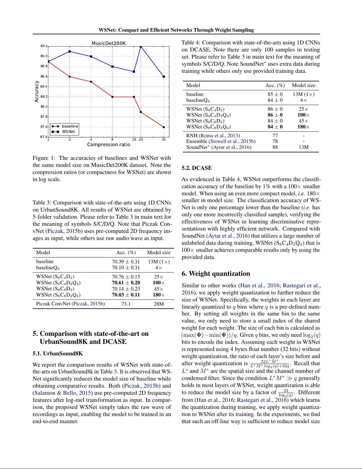
WSNet: Compact and Efficient Networks Thr ough W eight Sampling Xiaojie Jin 1 2 Y ingzhen Y ang 2 Ning Xu 2 Jianchao Y ang 3 Nebojsa Jojic 4 Jiashi Feng 1 Shuicheng Y an 5 1 Abstract W e present a new approach and a no vel architec- ture, termed WSNet, for learning compact and ef- ficient deep neural networks. Existing approaches con ventionally learn full model parameters inde- pendently and then compress them via ad hoc processing such as model pruning or filter factor - ization. Alternativ ely , WSNet proposes learning model parameters by sampling from a compact set of learnable parameters, which naturally enforces parameter sharing throughout the learning process. W e demonstrate that such a novel weight sampling approach (and induced WSNet) promotes both weights and computation sharing f av orably . By employing this method, we can more ef ficiently learn much smaller networks with competiti ve performance compared to baseline networks with equal numbers of con volution filters. Specifically , we consider learning compact and efficient 1D con volutional neural networks for audio classifi- cation. Extensiv e experiments on multiple audio classification datasets verify the effecti veness of WSNet. Combined with weight quantization, the resulted models are up to 180 × smaller and theo- retically up to 16 × faster than the well-established baselines, without noticeable performance drop. 1. Introduction Despite remarkable successes in various applications, deep neural networks (DNNs) usually suffer follo wing two prob- lems that stem from their inherent huge parameter space. First, most of state-of-the-art deep architectures are prone to ov er-fitting e ven when trained on lar ge datasets ( Simonyan & Zisserman , 2015 ; Szegedy et al. , 2015 ). Secondly , DNNs usually consume large amount of storage memory and en- ergy ( Han et al. , 2016 ), which makes it dif ficult to use them 1 National Univ ersity of Singapore, Singapore 2 Snap Inc. Re- search, Los Angeles, USA 3 Bytedance Inc., Menlo Park, USA 4 Microsoft Research, Redmond, USA 5 360 AI Institute, Beijing, China. Correspondence to: Xiaojie Jin < xjjin0731@gmail.com > . Pr oceedings of the 35 th International Confer ence on Machine Learning , Stockholm, Sweden, PMLR 80, 2018. Copyright 2018 by the author(s). in de vices with limited memory and power (such as portable devices or chips). Dif ferent from most existing works ( Han et al. , 2015 ; Li et al. , 2017 ; Jaderberg et al. , 2014 ; Lebede v et al. , 2014 ; Hinton et al. , 2015 ) on model compression and acceleration that ignore the strong dependencies among weights and learn filters independently based on existing network architectures, this paper proposes to explicitly en- force the parameter sharing among filters to more effecti vely learn compact and efficient deep netw orks. In this paper, we propose a W eight S ampling deep neu- ral network ( i.e. WSNet) to significantly reduce both the model size and computation cost, achie ving more than 100 × smaller size and up to 16 × speedup at negligible perfor- mance drop or e ven achie ving better performance than the baseline ( i.e. con v entional networks that learn filters inde- pendently). Specifically , WSNet is parameterized by layer - wise condensed filters from which each filter participating in actual con volutions can be directly sampled, in both spatial and channel dimensions. Since condensed filters ha ve signif- icantly fewer parameters than independently trained filters as in con ventional CNNs, learning by sampling from them makes WSNet a more compact model compared to con ven- tional CNNs. In addition, to reduce the ubiquitous computa- tional redundancy in con v olving the ov erlapped filters and input patches, we propose an inte gral image based method to dramatically reduce the computation cost of WSNet in both training and inference. The inte gral image method is also advantageous because it enables weight sampling with different filter size and minimizes computational overhead to enhance the learning capability of WSNet. In order to demonstrate the efficac y of WSNet, we con- duct extensi ve e xperiments on challenging audio classifica- tion tasks. On each test dataset, including ESC-50 ( Piczak , 2015a ), UrbanSound8K ( Salamon et al. , 2014 ), DCASE ( Stowell et al. , 2015 ) and MusicDet200K (a self-collected dataset, as detailed in Section 4 ), WSNet significantly re- duces the model size of the baseline by 100 × with com- parable or e ven higher classification accurac y . When com- pressing more than 180 × , WSNet is only subject to negligi- ble accuracy drop. At the same time, WSNet significantly reduces the computation cost (up to 16 × ). Such results strongly establish the capability of WSNet to learn compact and ef ficient networks. Last but not the least, we pro vide an intuitiv e method to extend WSNet from 1D CNNs to WSNet: Compact and Efficient Networks Through W eight Sampling 2D CNNs. Experimental results on MNIST and CIF AR10 strongly e vidence the potential capability of WSNet to learn efficient netw orks on 2D CNNs. 2. Related W orks 2.1. Deep Model Compression and Acceleration Recent works in network compression adopt weight prun- ing ( Han et al. , 2015 ; Collins & K ohli , 2014 ; Anw ar et al. , 2017 ; Lebede v & Lempitsky , 2016 ; Kim et al. , 2015 ; Luo et al. , 2017 ; Li et al. , 2017 ), filter decomposition ( Sindhw ani et al. , 2015 ; Denton et al. , 2014 ; Jaderberg et al. , 2014 ), hashed networks ( Chen et al. , 2015 ; 2016 ) and weight quan- tization ( Han et al. , 2016 ). Howe ver , although those works reduce model size, they also suf fer from large performance drop. Bucilu et al. ( 2006 ) and Ba & Caruana ( 2014 ) are based on student-teacher approches which may be dif ficult to apply in new tasks since they require training a teacher network in adv ance. Denil et al. ( 2013 ) predicts parameters based on a fe w number of weight v alues. Jin et al. ( 2016 ) proposes an iterative hard thresholding method, but only achiev e relati vely small compression ratios. Gong et al. ( 2014 ) uses a binning method which can only be applied ov er fully connected layers. Hinton et al. ( 2015 ) compresses deep models by transferring the knowledge from pre-trained larger netw orks to smaller networks. In terms of deep model acceleration, the factorization and quantization methods listed above can reduce computa- tion latenc y in inference. FFT ( Mathieu et al. , 2013 ) and LCNN ( Bagherinezhad et al. , 2016 ) are also used to speed up computation in pratice. Comparati vely , WSNet is supe- rior because it learns networks that ha ve both smaller model size and faster computation versus baselines. 2.2. Efficient Model Design WSNet presents a class of novel models with the appeal- ing properties of a small model size and small computation cost. Some recently proposed efficient model architectures include the class of Inception models ( Szegedy et al. , 2015 ; Ioffe & Szegedy , 2015 ; Chollet , 2016 ), the class of Resid- ual models ( He et al. , 2016 ; Xie et al. , 2017 ; Chen et al. , 2017 ) and the factorized networks which use fully f actorized con volutions. MobileNet ( Howard et al. , 2017 ) and Flat- tened networks ( Jin et al. , 2014 ) are based on factorization con volutions. ShuffleNet ( Zhang et al. , 2017 ) uses group con volution and channel shuffle to reduce computational cost. Compared with the abo ve works, WSNet presents a new model design strategy which is more fle xible and gen- eralizable: the parameters in deep networks can be obtained con veniently from a more compact representation through the proposed weight sampling method. 2.3. A udio classification Audio classification aims to classify the surrounding en- vironment where an audio stream is generated giv en the audio input ( Barchiesi et al. , 2015 ). Compared with other CNN based methods which use pre-computed features, e.g . MFCC ( Pols et al. , 1966 ; Davis & Mermelstein , 1980 ) and spectrogram ( Flanagan , 1972 ), recently proposed SoundNet ( A ytar et al. , 2016 ) yields significant the state-of-the-art re- sults by directly taking one dimensional raw wav e signals as input. In this paper , we demonstrate that the proposed WS- Net achiev es a comparable or ev en better performance than SoundNet at a significantly smaller size and faster speed. 3. Method 3.1. Notations Before diving into the details, we first introduce the nota- tions used in this paper . The traditional 1D conv olution layer takes as input the feature map F ∈ R T × M and produces an output feature map G ∈ R T × N where ( T , M , N ) denotes the spatial length of input, the channel of input and the num- ber of filters respecti vely . W e assume that the output has the same spatial size as input which holds true by using zero padded con volution. The 1D con v olution kernel K used in the actual con volution of WSNet has the shape of ( L, M , N ) where L is the kernel size. Let k n , n ∈ { 1 , · · · N } denotes a filter and f t , t ∈ { 1 , · · · T } denotes a input patch that spatially spans from t to t + L − 1 , then the con volution assuming stride one and zero padding is computed as: G t,n = f t · k n = L − 1 X l =0 M − 1 X m =0 F t + l,m × K l,m,n , (1) where · stands for the vector inner product. Note we omit the element-wise activ ation function to simplify the notation. In WSNet, instead of learning each weight independently , K is obtained by sampling from a learned condensed filter Φ which has the shape of ( L ∗ , M ∗ ) . The goal of training WSNet is thus cast to learn more compact DNNs which satisfy the condition of L ∗ M ∗ < LM N . WSNet uses a condensed filter per con volutional layer . T o quantize the advantage of WSNet in achieving compact networks, we define the compactness of K in a learned layer in WSNet w .r .t. the con ventional layer with independently learned weights as: compactness = LM N L ∗ M ∗ . (2) In the following section, we demonstrate WSNet learn com- pact networks by sampling weights in two dimensions: the spatial dimension and the channel dimension. WSNet: Compact and Efficient Networks Through W eight Sampling Channel Sampling Spatial Sampling Sampling Stride: S Shapes of Filters Figure 1: Illustration of WSNet that learns small condensed filters with weight sampling along two dimensions: spatial dimension (the bottom panel) and channel dimension (the top panel). The figure depicts procedure of generating two continuous filters (in pink and purple respectiv ely) that con volve with input. In spatial sampling , filters are extracted from the condensed filter with a stride of S . In channel sampling , the channel of each filter is sampled repeatedly for C times to achieve equal with the input channel. Please refer to Section 3.2 for detailed explanations. All figures in this paper are best viewed in zoomed-in pdf. 3.2. W eight sampling 3 . 2 . 1 . A LO N G S PA T I A L D I M E N S I O N In con ventional CNNs, the filters in a layer are learned in- dependently which presents two disadv antages. Firstly , the resulted DNNs have a large number of parameters, which im- pedes their deployment in computation resource constrained platforms. Second, such o ver -parameterization makes the network prone to overfitting and getting stuck in (e xtra intro- duced) local minima. T o solve these two problems, a nov el weight sampling method is proposed to efficiently reuse the weights among filters. Specifically , in each con volutional layer of WSNet, all conv olutional filters K are sampled from the condensed filter Φ , as illustrated in Figure 1 . By scanning the weight sharing filter with a windo w size of L and stride of S , we could sample out N filters with filter size of L . Formally , the equation between the filter size of the condensed filter and the sampled filters is: L ∗ = L + ( N − 1) S. (3) The compactness along spatial dimension is LM ∗ N L ∗ M ∗ ≈ L S . Note that since the minimal value of S is 1, the minimal value of L ∗ ( i.e. the minimum spatial length of the con- densed filter) is L + N − 1 and the maximal achievable compactness is therefore L . 3 . 2 . 2 . A L O N G C H A N N E L D I M E N S I O N Although it is experimentally verified that the weight sam- pling strategy could learn compact deep models with ne g- ligible loss of classification accuracy (see Section 4 ), the maximal compactness is limited by the filter size L , as men- tioned in Section 3.2.1 . In order to seek more compact networks without such limi- tation, we propose a channel sharing strategy for WSNet to learn by weight sampling along the channel dimension. As illustrated in Figure 1 (top panel), the actual filter used in con volution is generated by repeating sampling for C times. The relation between the channels of filters before and after channel sampling is: M = M ∗ × C , (4) Therefore, the compactness of WSNet along the channel dimension achie ves C . As introduced later in Experiments (Section 4 ), we observe that the repeated weight sampling along the channel dimension significantly reduces the model size of WSNet without significant performance drop. One notable adv antage of channel sharing is that the maximum compactness can be as large as M ( i.e. when the condensed filter has channel of 1), which paves the way for learning much more aggressiv ely smaller models ( e.g. more than 100 × smaller models than baselines). W e attrib ute the ef- fectiv eness of channel sharing to reducing the redundancy along the channel dimension, especially in top layers. In general architecture design, the number of filter channels grows linearly with the layer depth. Ho wev er , the spatial size of kernels becomes smaller or remains unchanged. This implies redundancy in higher layers mainly come from the channel dimension. The above analysis for weight sampling along spa- tial/channel dimensions can be conv eniently generalized from conv olution layers to fully connected layers. For a fully connected layer , we treat its weights as a flattened vec- tor with channel of 1, along which the spatial sampling (ref. Section 3.2.1 ) is performed to reduce the size of learnable parameters. For more details, please refer the supplementary material. 3 . 2 . 3 . T H E T R A I N I N G O F C O N D E N S E D FI LT E R S WSNet is trained from the scratch in a similar way to con- ventional deep con v olutional networks by using standard error back-propagation. Since every weight K l,m,n in the con volutional kernel K is sampled from the condensed filter Φ along the spatial and channel dimension, the only dif fer- ence is the gradient of Φ i,j is the summation of all gradients of weights that are tied to it. Therefore, by simply recording the position mapping M : ( i, j ) → ( l , m, n ) from Φ i,j to all the tied weights in K , the gradient of Φ i,j is calculated as: ∂ L ∂ Φ i,j = X s ∈M ( i,j ) ∂ L ∂ K s (5) where L is the con ventional cross-entropy loss function. In open-sourced machine learning libraries which represent computation as graphs, such as T ensorFlo w ( Abadi et al. , 2016 ), Equation ( 5 ) can be calculated automatically . WSNet: Compact and Efficient Networks Through W eight Sampling v 2 ... I (u 1 + L -1,v 1 + L -1) I (u 1 ,v 1 ) v 2 + L -1 v 1 + L -1 u 2 u 1 + L -1 u 2 + L -1 v 1 u 1 Figure 2: Illustration of ef ficient computation with integral image in WSNet. The inner product map P ∈ R T × L ∗ calculates the inner product of each row in F and each column in Φ as in Eq. ( 7 ) . The con volution result between a filter k 1 which is sampled from Φ and the input patch f 1 is then the summation of all values in the segment between ( u, v ) and ( u + L − 1 , v + L − 1) in P (recall that L is the con volutional filter size). Since there are repeated calculations when the filter and input patch are o verlapped, e .g. the green segment indicated by arrow when performing conv olution between k 2 and s 2 , we construct the integral image I using P according to Eq. ( 8 ) . Based on I , the con volutional results between any sampled filter and input patch can be retrieved directly in time complexity of O(1) according to Eq. ( 9 ) , e.g. the results of k 1 · s 1 is I ( u 1 + L − 1 , v 1 + L − 1) − I ( u 1 − 1 , v 1 − 1) . For notation definitions, please refer to Sec. 3.1 . The comparisons of computation costs between WSNet and the baselines using con ventional architectures are introduced in Section 3.4 . 3.3. Denser W eight Sampling The performance of WSNet might be adversely affected when the size of condensed filter is decreased aggressi vely ( i.e. when S and C are large). T o enhance the learning capability of WSNet, we could sample more filters from the condensed filter . Specifically , we use a smaller sampling stride ¯ S ( ¯ S < S ) when performing spatial sampling. In or- der to k eep the shape of weights unchanged in the follo wing layer , we append a 1 × 1 con volution layer with the shape of (1 , ¯ n, n ) to reduce the channels of densely sampled filters. It is experimentally verified that denser weight sampling can ef fectiv ely improve the performance of WSNet in Sec- tion 4 . Howe ver , since it also brings extra parameters and computational cost to WSNet, denser weight sampling is only used in lo wer layers of WSNet whose filter number ( n ) is small. Besides, one can also conduct channel sampling on the added 1 × 1 con volution layers to further reduce their sizes. 3.4. Efficient Computation with integral image According to Equation 1 , the computation cost in terms of the number of multiplications and adds ( i.e. Mult-Adds) in a con ventional con volutional layer is: T M LN (6) Howe ver , as illustrated in Figure 2 , since all filters in a layer in WSNet are sampled from a condensed filter Φ with stride S , calculating the results of conv olution in the channel wrapping v 2 + L -1 v 1 + L -1 u 1 + L -1 u 2 + L -1 v 1 v 2 u 1 u 2 Figure 3: A variant of the integral image method used in practice which is more efficient than that illustrated in Figure 2 . Instead of repeatedly sampling along the channel dimension of Φ to con volv e with the input F , we wrap the channels of F by summing up C matrixes that are evenly divided from F along the channels, i.e. ˜ F ( i, j ) = P C − 1 c =0 F ( i, j + cM ∗ ) . Since the channle of ˜ F is only 1 /C of the channel of F , the ov erall computation cost is reduced as demonstrated in Eq. ( 11 ). con ventional way as in Eq. ( 1 ) incurs sev ere computational redundancies. Concretely , as can be seen from Eq. ( 1 ) , one item in the ouput feature map is equal to the summation of L inner products between the row v ector of f and the column vector of k . Therefore, when two overlapped filters that are sampled from the condensed filter ( e.g. k 1 and k 2 in Fig. 2 ) con volv es with the ov erlapped input windo ws ( e.g . f 1 and f 2 in Fig. 2 )), some partially repeated calculations exist ( e.g. the calculations highlight in green and indicated by arrow in Fig. 2 ). T o eliminate such redundancy in con volution and speed-up WSNet, we propose a novel integral image method to enable efficient computation via sharing computations. W e first calculate an inner product map P ∈ R T × L ∗ which stores the inner products between each row vector in the input feature map ( i.e. F ) and each column v ector in the condensed filter ( i.e. Φ ): P ( u, v ) = ( F u, : · Φ : ,v , u ∈ [0 , T − 1] and v ∈ [0 , L ∗ − 1] 0 , other w ise. (7) The integral image for speeding-up con volution is denoted as I . It has the same size as P and can be con veniently obtained throught below formulation: I ( u, v ) =      I ( u − 1 , v − 1) + P ( u, v ) , u > 0 , v > 0 P ( u, 0) , v = 0 P (0 , v ) , u = 0 (8) Based on I , all con volutional results can be obtained in time complexity of O (1) as follo ws G t,n = I ( t + L − 1 , nS + L − 1) − I ( t − 1 , nS − 1) (9) Recall that the n -th filter lies in the spatial range of ( nS, nS + L − 1) in the condensed filter Φ . Since G ∈ WSNet: Compact and Efficient Networks Through W eight Sampling R T × N , it thus takes T N times of calculating Eq. ( 9 ) to get G . In Eq. ( 7 ) ∼ Eq. ( 9 ) , we omit the case of padding for clear description. When zero padding is applied, we can freely get the con volutional results for the padded areas e ven without using Eq. ( 9 ) since I ( u, v ) = I ( T , v − 1) , u > T . Based on Eq. ( 7 ) ∼ Eq. ( 9 ) , the computation cost of the proposed integral image method is T M L ∗ | {z } Eq. ( 7 ) + T L ∗ | {z } Eq. ( 8 ) + T N |{z} Eq. ( 9 ) = T ( M + 1) L ∗ + T N . (10) Note the computation cost of P ( i.e. Eq. ( 7 ) ) is the dominat- ing term in Eq. ( 10 ) . Based on Eq. ( 6 ) , Eq. ( 10 ) and Eq. ( 3 ) , the theoretical acceleration ratio is T M LN T ( M + 1) L ∗ + T N ≈ L S Recall that L is the filter size and S is the pre-defined stride when sampling filters from the condensed filter Φ (ref. to Eq. ( 3 )). In practice, we adopt a variant of the abov e method to further boost the computation efficienc y of WSNet, as illustrated in Fig 3 . In Eq. ( 7 ) , we repeat Φ by C times along the channel dimension to make it equal with the channel of the input F . Howe ver , we could first wrap the channels of F by accumulating the values with interval of L along its channel dimension to a thinner feature map ˜ F ∈ R T × M ∗ which has the same channel number as Φ , i.e. ˜ F ( i, j ) = P C − 1 c =0 F ( i, j + cM ∗ ) . Both Eq. ( 8 ) and Eq. ( 9 ) remain the same. Then the computational cost is reduced to T M ∗ ( C − 1) | {z } channel warp + T M ∗ L ∗ | {z } Eq. ( 7 ) + T L ∗ | {z } Eq. ( 8 ) + T N |{z} Eq. ( 9 ) (11) where the first item is the computational cost of warping the channels of F to obtain ˜ F . Since the dominating term ( i.e. Eq. ( 7 ) ) in Eq ( 11 ) is smaller than in Eq. ( 10 ) , the overall computation cost is thus largely reduced. By combining Eq. ( 11 ) and Eq. ( 6 ) , the theoretical acceleration compared to the baseline is M LN M ∗ ( C + L ∗ − 1) + ( L ∗ + N ) (12) Finally , we note that the integral image method applied in WSNet naturally takes adv antage of the property in weight sampling: redundant computations exist between ov erlapped filters and input patches. Different from other deep model speedup methods ( Sindhwani et al. , 2015 ; Den- ton et al. , 2014 ) which require to solve time-consuming optimization problems and incur performance drop, the in- tegral image method can be seamlessly embeded in WSNet without negati vely affecting the final performance. 3.5. An Intuitive Extension of WSNet fr om 1D con vnet to 2D con vnet In this paper , we focus on WSNet with 1D con vnets. Com- prehensiv e experiments clearly demonstrate its advantages in learning compact and computation-ef ficient networks. W e note that WSNet is general and can also be applied to build 2D con vnets. In 2D con vnets, each filter has three di- mensions including two spatial dimensions ( i.e . along X and Y directions) and one channel dimension. One straightfor - ward extension of WSNet to 2D con vnets is as follows: for spatial sampling, each filter is sampled out as a patch (with the same number of channels as in condensed filter) from condensed filter . Channel sampling remains the same as in 1D con vnets, i.e. repeat sampling in the channel dimension of condensed filter . Follo wing the notations for WSNet with 1D con vnets (ref. to Sec. 3.1 ), we denote the filters in one layer as K ∈ R w × h × M × N where ( w , h, M , N ) denote the width and height of each filter , the number of channels and the number of filters respectiv ely . The condensed filter Φ has the shape of ( W , H, M ∗ ) . The relations between the shape of condensed filter and each sampled filter are: W = w + ( d √ N e − 1) S w H = h + ( d √ N e − 1) S h M = M ∗ × C (13) where S w and S h are the sampling strides along two spa- tial dimensions and C is the compactness of WSNet along channel dimension. The compactnesses (ref. to Eq. ( 2 ) for denifinition) of WSNet along spatial and channel dimension are W H whN and C respecti vely . Howe ver , such straightforward extension of WSNet to 2D con vnets may not be optimum and we belie ve there are more sophisticated and ef fectiv e methods for applying WSNet to 2D convnets and we would like to e xplore in our future work. Ne vertheless, we con- duct preliminary experiments on 2D con vents using abo ve intuitiv e extension and verify the ef fectiv eness of WSNet in image classification tasks (on MNIST and CIF AR10). 4. Experiments 4.1. Experimental Settings Datasets and baseline networks W e collect a lar ge-scale music detection dataset (MusicDet200K) from publicly av ailable platforms ( e.g. Facebook, T witter , etc. ) for con- ducting experiments. For fair comparison with previous literatures, we also test WSNet on three standard, publicly av ailable datasets, i.e ESC-50, UrbanSound8K and DCASE. Due to space limit, please refer to the details of used datasets in supplementary material. T o test the scability of WSNet to dif ferent network archi- tectures ( e.g . whether having fully connected layers or not), WSNet: Compact and Efficient Networks Through W eight Sampling T able 1: Baseline-1: configurations of the baseline network used on MusicDet200K. Each con volutional layer is follo wed by a nonlinearity layer ( i.e. ReLU), batch normalization layer and pooling layer , which are omitted in the table for brevity . The strides of all pooling layers are 2. The padding strategies adopted for both conv olutional layers and fully connected layers are all “size preserving”. Layer con v1 con v2 con v3 con v4 con v5 con v6 con v7 fc1 fc2 Filter sizes 32 32 16 8 8 8 4 1536 256 #Filters 32 64 128 128 256 512 512 256 128 Stride 2 2 2 2 2 2 2 1 1 #Params 1K 65K 130K 130K 260K 1M 1M 390K 33K #Mult-Adds ( 10 8 ) 4.1 65.5 32.7 8.2 4.1 4.2 1.0 0.1 0.007 T able 2: Baseline-2: configuration of the baseline network used on ESC-50, UrbanSound8K and DCASE. This baseline is adapted from SoundNet ( A ytar et al. , 2016 ) by applying pooling layers to all but the last con volutional layer . For bre vity , the nonlinearity layer ( i.e. ReLU), batch normalization layer and pooling layer follo wing each con volutional layer are omitted. The kernel sizes for pooling layers following con v1-con v4 and conv5-con v7 are 8 and 4 respectiv ely . The stride of ev ery pooling layers is 2. Layer con v1 con v2 con v3 con v4 con v5 con v6 con v7 con v8 Filter sizes 64 32 16 8 4 4 4 8 #Filters 16 32 64 128 256 512 1024 1401 Stride 2 2 2 2 2 2 2 2 #Params 1K 16K 32K 65K 130K 520K 2M 11M #Mult-Adds ( 10 8 ) 2.3 9.0 4.5 2.3 1.2 1.2 1.2 2.3 T able 3: Ablati ve study of the ef fects of dif ferent settings of WSNet on the model size, computation cost (in terms of #mult-adds) and classification accurac y on ESC-50. For clear description, we name WSNets with dif ferent settings by the combination of symbols S/C/D/Q. “S” denotes the weight sampling along spatial dimension; “C” denotes the weight sampling along the channel dimension. “D” denotes denser filter sampling. “Q” denotes weight quantization. The numbers in subscripts of S/C/D/Q denotes the maximum compactness (ref. to Sec. 3.1 for the definition of compactness) on spatial/channel dimension in all layers, the ratio of the number of filters in WSNet versus in the baseline and the ratio of WSNet’ s size before and after weight quantization, respecti vely . The model size and the computational cost are provided for the baseline. F or the model size and #mult-adds of WSNet, we provide the ratio of the baseline’ s model size versus WSNet’ s model size and the ratio of the baseline’ s #Mult-Adds versus WSNet’ s #Mult-Adds. WSNet’ s con v { 1-4 } conv5 con v6 conv7 conv8 Acc. Model Mult-Adds settings S C D S C D S C D S C D S C D size Baseline 1 1 1 1 1 1 1 1 1 1 1 1 1 1 1 66.0 ± 0.2 13M (1 × ) 2.4e8 (1 × ) BaselineQ 4 1 1 1 1 1 1 1 1 1 1 1 1 1 1 1 65.7 ± 0.2 4 × 1 × S 2 2 1 1 2 1 1 2 1 1 2 1 1 2 1 1 66.6 ± 0.3 2 × 1 × S 4 4 1 1 4 1 1 4 1 1 4 1 1 4 1 1 66.3 ± 0.1 4 × 1.6 × S 8 8 1 1 4 1 1 4 1 1 4 1 1 8 1 1 65.2 ± 0.1 7 × 4.7 × C 2 1 2 1 1 2 1 1 2 1 1 2 1 1 2 1 66.8 ± 0.2 2 × 1 × C 4 1 4 1 1 4 1 1 4 1 1 4 1 1 4 1 66.5 ± 0.3 4 × 1.6 × C 8 1 8 1 1 4 1 1 4 1 1 4 1 1 8 1 65.8 ± 0.3 8 × 2.8 × S 4 C 4 4 4 1 4 4 1 4 4 1 4 4 1 4 4 1 65.6 ± 0.3 16 × 6.3 × S 8 C 8 4 4 1 4 8 1 4 8 1 4 8 1 8 8 1 65.2 ± 0.3 60 × 18.1 × S 8 C 4 D 2 4 4 2 4 4 1 4 4 1 4 4 1 8 4 1 66.5 ± 0.1 25 × 2.3 × S 8 C 4 D 2 Q 4 4 4 2 4 4 1 4 4 1 4 4 1 8 4 1 66.2 ± 0.1 100 × 2.3 × S 8 C 8 D 2 4 4 1 4 8 1 4 8 1 4 8 1 8 8 1 66.1 ± 0.0 45 × 2.4 × S 8 C 8 D 2 Q 4 4 4 2 4 8 1 4 8 1 4 8 1 8 8 1 65.8 ± 0.0 180 × 2.4 × WSNet: Compact and Efficient Networks Through W eight Sampling two baseline networks are used in comparision. Their archi- tectures are shown in T able 1 and T able 2 respectiv ely . Evaluation criteria T o demonstrate that WSNet is capa- ble of learning more compact and efficient models than con ventional CNNs, three e valuation criteria are used in our experiments: model size, the number of multiply and adds in calculation (mult-adds) and classification accurac y . For the results of WSNet models, we also gi ve the std of fi ve different runs. Implementation details WSNet is implemented and trained from scratch in T ensorflow ( Abadi et al. , 2016 ). Fol- lowi ng ( A ytar et al. , 2016 ), the Adam ( Kingma & Ba , 2014 ) optimizer , a fixed learning rate of 0.001, and momentum term of 0.9 and batch size of 64 are used throughout experi- ments. W e initialized all the weights to zero mean gaussian noise with a standard deviation of 0.01. In the network used on MusicDet200K, the dropout ratio for the dropout layers ( Sri vasta va et al. , 2014 ) after each fully connected layer is set to be 0.8. The overall training takes 100,000 iterations. 4.2. Results and analysis 4 . 2 . 1 . E S C - 5 0 Ablation analysis W e in vestigate the effects of each com- ponent in WSNet on the model size, computational cost and classification accuracy . The comparativ e study results of different settings of WSNet are listed in T able 3 . For clear description, we name WSNets with dif ferent settings by the combination of symbols S/C/D/Q. Please refer to the caption of T able 3 for detailed meanings. (1) Spatial sampling. W e test the performance of WS- Net by using dif ferent sampling stride S in spatial sampling. As listed in T able 3 , S 2 and S 4 slightly outperforms the classification accuracy of the baseline, possibly due to re- ducing the ov erfitting of models. When the sampling stride is 8, i.e. the compactness in spatial dimension is 8 (ref. to Section 3.2.1 ), the classification accuracy of S 8 only drops by 0.6%. Note that the maximum compactness along the spatial dimension is equal to the filter size, thus for the layer “conv { 5-7 } ” which hav e filter sizes of 4, their com- pactnesses are limited by 4 (highlighted by underlines in T able 3 ). Abov e results clearly demonstrate that the spa- tial sampling enables WSNet to learn significantly smaller model with comparable accuracies w .r .t. the baseline. (2) Channel sampling. Three different compactness along the channel dimension, i.e . 2, 4 and 8 are tested by comparing with baslines. It can be observed from T a- ble 3 that C 2 and C 4 and C 8 hav e linearly reduced model size without incurring noticeable drop of accurac y . In fact, C 2 and C 4 can ev en improve the accurac y upon baselines, demonstrating the effecti veness of channel sampling in WS- Net. When learning more compact models, C 8 demonstrates better performance compared to S 8 that has the same com- pactness in the spatial dimension, which suggests we should focus on the channel sampling when the compactness along the spatial dimension is high. W e then simultaneously perform weight sampling on both the spatial and channel dimensions. As demonstrated by the results of S 4 C 4 and S 8 C 8 , WSNet can learn highly compact models without significant performance drop (less than 1%). (3) Denser weight sampling. Denser weight sampling is used to enhance the learning capability of WSNet with aggressiv e compactness ( i.e. when S and C are large) and make up the performance loss caused by sharing too much parameters among filters. As sho wn in T able 3 , by sampling 2 × more filters in con v { 1-4 } , S 8 C 8 D 2 significantly outper- forms the S 8 C 8 . Abov e results demonstrate the effecti veness of denser weight sampling to boost the performance. (4) Inte gral imag e for efficient computation. As evi- denced in the last column in T able 3 , the proposed integral image method consistently reduces the computation cost of WSNet. For S 8 C 8 which is 60 × smaller than the baseline, the computation cost (in terms of #mult-adds) is signifi- cantly reduced by 18.1 times. Due to the extra computation cost brought by the 1 × 1 con volution in denser filter sam- pling, S 8 C 8 D 2 achiev es lo wer acceleration (2.4 × ). Group con volution ( Xie et al. , 2017 ) can be used to alle viate the computation cost of the added 1 × 1 con volution layers. W e will explore this direction in our future work. (5) W eight quantization. It can be observed from T a- ble 3 that by using 256 bins to represent each weight by one byte ( i.e. 8bits), S 8 C 8 D 2 Q 4 and S 8 C 4 D 2 Q 4 hav e much smaller model size compared with baselines while incurring negligible accuracy loss. The abo ve result demonstrates that the weight quantization is complementary to WSNet and they can be used jointly to effecti vely reduce the model size of WSNet. Please ref. to supplementary material for the details of the weight quantization methods. (6) WSNet versus narrowed baselines. T o further verify WSNet’ s capacity of learning compact models, we compare WSNet with baselines compressed in an intuiti ve way , i.e. re- ducing the number of filters in each layer . If #filters in each layer is reduced by T , the ov erall #parameters in baselines is reduced by T 2 ( i.e. the compression ratio of model size is T 2 ). In Figure 4 , we plot ho w baseline accuracy varies with respect to dif ferent compression ratios and the accuracies of WSNet with the same model size of compressed baselines. As shown in Figure 4 , WSNet outperforms baselines by a large margin across all compression ratios. Particularly , when the compression ratios are large ( e .g. 45), base- lines suffer severe performance drop. In contrast, WS- WSNet: Compact and Efficient Networks Through W eight Sampling 1 2 4 8 16 20 45 Compression ratio 60 61 62 63 64 65 66 67 68 Accuracy ESC-50 baseline WSNet Figure 4: The accuracies of baselines and WSNet with the same model size on ESC-50 dataset. Note the compression ratios (or compactness for WSNet) are shown in log scale. Net achiev es comparable accuracies with full-size baselines (66.1 versus 66.0). This clearly demonstrates the ef fectiv e- ness of weight sampling methods proposed in WSNet. In supplementary material, we also present the comparison between WSNet and narrowed baselines on MusicDet200K. 4 . 2 . 2 . C O M PA R I S O N W I T H S TA T E - O F - T H E - A RT The comparison of WSNet with other state-of-the-arts on ESC-50 is listed in T able 4 . Compared with the SoundNet trained with provided data, WSNets significantly outper- form its classification accurac y by o ver 10% with more than 100 × smaller models. After pre-training using a large num- ber of unlabeled videos, SoundNet ∗ achie ves better accurac y than WSNet. Howe ver , since the unsupervised pre-training method is orthogonal to WSNet, we believ e that WSNet can achiev e better performance by training in a similar way as SoundNet ( A ytar et al. , 2016 ) on a large amount of un- labeled video data. Due to space limit, for experimental results on other datasets as well as the ablative study on MusicDet200K, please refer to supplementary material. 4.3. Discussions W e argue that there are tw o reasons for the success of WS- Net: (1) The epitome methods ( Beno ˆ ıt et al. ; Aharon & Elad , 2008 ; Jojic et al. ) have been successfully deplo yed in sparse coding literatures, where the coding dictionaries are formed by ov erlapping patches in the epitome which has few free parameters. This indicates effecti ve representations of com- plex signals can be generated from a lo w-dimensional space (with high parameter efficiency). It thus motiv ates us to learn compact (or epitomic) filters in deep neural networks, i.e. all filters which participate in the actual conv olution are generated from the condensed filters. (2) W eight quantiza- tion techniques were successfully applied for compressing deep models where multiple weights are encoded into the T able 4: Comparison with state-of-the-arts using 1D CNNs on ESC-50. All results of WSNet are obtained by 10-folder valida- tion. Please refer to T able 3 for the meaning of symbols S/C/D/Q. SoundNet ∗ use extra training data while other methods use only provided training data. Model Acc. (%) Model size Piczak Con vNet ( Piczak , 2015b ) 64.5 28M SoundNet ( A ytar et al. , 2016 ) 51.1 13M SoundNet ∗ ( A ytar et al. , 2016 ) 72.9 13M WSNet (S 8 C 4 D 2 ) 66.5 ± 0.10 0.52M WSNet (S 8 C 4 D 2 Q 4 ) 66.25 ± 0.25 0.13M WSNet (S 8 C 8 D 2 ) 66.1 ± 0.15 0.29M WSNet (S 8 C 8 D 2 Q 4 ) 65.8 ± 0.25 0.07M T able 5: T est error rates (in %) of WSNet and HashNet on CI- F AR10 and MNIST . The baselines used for MNIST/CIF AR10 are simple 3-layer fully connected network and 5-layer con volutional network respecti vely . The model size is provided for the base- line. For the model size of WSNet/HashNet, we provide the ratio ( i.e. n ) of the baseline’ s model size versus the model size of WS- Net/HashNet. For WSNet, we set the layer -wise compactness to be n . Specifically , for each con volutional layer in WSNet, we set its compactness along spatial/channel dimension to be √ n/ √ n , respectiv ely . Model Model size Error rate Model size Error rate CIF AR10 MNIST baseline 1.2M ( × ) 14.91 800K (1 × ) 1.37 HashNet 16 × 21.42 8 × 1.43 HashNet 64 × 30.79 64 × 2.41 WSNet 16 × 17.82 8 × 1.29 WSNet 64 × 23.59 64 × 1.97 same value. WSNet goes further to overcome limitations of existing quantization methods through capturing the com- mon correlations among learned filters. For example, filters of the first layer in SoundNet ( A ytar et al. , 2016 ) (as illus- trated in Figure 5 in ( A ytar et al. , 2016 )) all learn similar constituent patterns, e.g. the descending/ascending slope lines. The proposed weight sampling method enables WS- Net to learn shared patterns by explicitly sampling filters from the condensed filter with overlapping. At the same time, the non-overlapped parts of sampled filters are able to learn different features which endows WSNet with strong learning capabilities. This is the main r eason that why WS- Net can learn much smaller networks without noticeable performance drop compared to baselines. Moreover , as the sampled filters are overlapped, we could use an integral im- age based method to speed up WSNets (ref. to Section 3.4 ). In this way , WSNet is able to learn both smaller and faster networks ef fectiv ely . WSNet: Compact and Efficient Networks Through W eight Sampling 4.4. Experimental results of WSNet on 2D CNNs Since both WSNet and HashNet ( Chen et al. , 2015 ; 2016 ) explore weights tying, we compare them on MNIST and CIF AR10. For fair comparison, we use the same baselines used in ( Chen et al. , 2015 ; 2016 ). All hyperparameters during training follo w ( Chen et al. , 2015 ; 2016 ). F or each dataset, we hold out 20% of training samples to form a validation set. The comparison results between WSNet and HashNet on MNIST/CIF AR10 are listed in T able 5 , from which one can observe that when learning networks with the same sizes, WSNet achie ves significantly lo wer error rates than HashNet on both datasets. Abov e results clearly demonstrate the adv antages of WSNet in learning compact models. Furthermore, we also conduct e xperiment on CIF AR10 with the state-of-the-art ResNet50 ( He et al. , 2016 ) as baseline. ResNet50 achiev es top-1 accuracy of 93.03% with #params of 0.85M. For WSNet, we set S w = S h = 2 and C = 4 . The experimental settings follo w those in ( He et al. , 2016 ). WSNet is able to achiev e 9 × smaller model size with slight performance drop ( 0.5% ). Such promising results further demonstrate the effecti veness of WSNet. 5. Conclusion In this paper, we present a class of W eight S ampling net- works (WSNet) which are highly compact and ef ficient. A nov el weight sampling method is proposed to sample fil- ters from condensed filters which are much smaller than the independently trained filters in con ventional netw orks. The weight sampling in conducted in two dimensions of the condensed filters, i.e . by spatial sampling and channel sampling. T aking advantage of the ov erlapping property of the filters in WSNet, we propose an integral image method for ef ficient computation. Extensive experiments on four audio classification datasets including MusicDet200K, ESC- 50, UrbanSound8K and DCASE clearly demonstrate that WSNet can learn compact and efficient netw orks with com- petitiv e performance. References Abadi, Mart ´ ın, Agarwal, Ashish, Barham, P aul, Brevdo, Eugene, Chen, Zhifeng, Citro, Craig, Corrado, Greg S, Da vis, Andy , Dean, Jef frey , Devin, Matthieu, et al. T ensorflow: Large-scale machine learning on heterogeneous distributed systems. arXiv pr eprint arXiv:1603.04467 , 2016. Aharon, Michal and Elad, Michael. Sparse and redundant model- ing of image content using an image-signature-dictionary . SIAM Journal on Ima ging Sciences , 1(3):228–247, 2008. Anwar , Sajid, Hwang, Kyuyeon, and Sung, W onyong. Structured pruning of deep con volutional neural networks. J. Emer g. T ech- nol. Comput. Syst. , 13(3):32:1–32:18, February 2017. ISSN 1550-4832. doi: 10.1145/3005348. URL http://doi.acm. org/10.1145/3005348 . A ytar, Y usuf, V ondrick, Carl, and T orralba, Antonio. Soundnet: Learning sound representations from unlabeled video. In NIPS , 2016. Ba, Jimmy and Caruana, Rich. Do deep nets really need to be deep? In NIPS , 2014. Bagherinezhad, Hessam, Rastegari, Mohammad, and Farhadi, Ali. Lcnn: Lookup-based con volutional neural network. arXiv pr eprint arXiv:1611.06473 , 2016. Barchiesi, Daniele, Giannoulis, Dimitrios, Stowell, Dan, and Plumbley , Mark D. Acoustic scene classification: Classify- ing en vironments from the sounds the y produce. IEEE Signal Pr ocessing Magazine , 32(3):16–34, 2015. Beno ˆ ıt, Louise, Mairal, Julien, Bach, Francis, and Ponce, Jean. Sparse image representation with epitomes. In CVPR . Bucilu, Cristian, Caruana, Rich, and Niculescu-Mizil, Alexandru. Model compression. In KDD , 2006. Cai, Rui, Lu, Lie, Hanjalic, Alan, Zhang, Hong-Jiang, and Cai, Lian-Hong. A flexible frame work for ke y audio effects detection and auditory context inference. IEEE T ransactions on audio, speech, and languag e pr ocessing , 14(3):1026–1039, 2006. Chen, W enlin, W ilson, James, T yree, Stephen, W einberger , Kilian, and Chen, Y ixin. Compressing neural networks with the hashing trick. In ICML , 2015. Chen, W enlin, Wilson, James T , T yree, Stephen, W einberger , Kil- ian Q, and Chen, Y ixin. Compressing conv olutional neural networks in the frequency domain. In KDD , 2016. Chen, Y unpeng, Li, Jianan, Xiao, Huaxin, Jin, Xiaojie, Y an, Shuicheng, and Feng, Jiashi. Dual path networks. arXiv pr eprint arXiv:1707.01629 , 2017. Chollet, Fran c ¸ ois. Xception: Deep learning with depthwise sepa- rable con volutions. arXiv preprint , 2016. Chu, Selina, Narayanan, Shrikanth, Kuo, C-C Jay , and Mataric, Maja J. Where am i? scene recognition for mobile robots using audio features. In ICME , 2006. Collins, Maxwell D and Kohli, Pushmeet. Memory bounded deep con volutional networks. arXiv preprint , 2014. Davis, Ste ven and Mermelstein, Paul. Comparison of parametric representation for monosyllabic word recognition in continu- ously spoken sentences. IEEE T rans. ASSP , Aug. 1980. Denil, Misha, Shakibi, Babak, Dinh, Laurent, de Freitas, Nando, et al. Predicting parameters in deep learning. In NIPS , 2013. Denton, Emily L, Zaremba, W ojciech, Bruna, Joan, LeCun, Y ann, and Fergus, Rob . Exploiting linear structure within conv olu- tional networks for ef ficient ev aluation. In NIPS , 2014. Flanagan, James L. Speech analysis, synthesis and perception. Springer - V erlag , 1972. Gong, Y unchao, Liu, Liu, Y ang, Ming, and Bourdev , Lubomir . Compressing deep con volutional networks using v ector quanti- zation. arXiv preprint , 2014. WSNet: Compact and Efficient Networks Through W eight Sampling Han, Song, Pool, Jeff, T ran, John, and Dally , William. Learning both weights and connections for efficient neural netw ork. In NIPS , 2015. Han, Song, Mao, Huizi, and Dally , W illiam J. Deep compres- sion: Compressing deep neural network with pruning, trained quantization and huffman coding. In ICLR , 2016. He, Kaiming, Zhang, Xiangyu, Ren, Shaoqing, and Sun, Jian. Deep residual learning for image recognition. In CVPR , 2016. Hinton, Geoffrey , V inyals, Oriol, and Dean, Jeff. Distill- ing the knowledge in a neural network. arXiv pr eprint arXiv:1503.02531 , 2015. How ard, Andrew G, Zhu, Menglong, Chen, Bo, Kalenichenko, Dmitry , W ang, W eijun, W eyand, T obias, Andreetto, Marco, and Adam, Hartwig. Mobilenets: Ef ficient con volutional neu- ral networks for mobile vision applications. arXiv pr eprint arXiv:1704.04861 , 2017. Ioffe, Sergey and Szegedy , Christian. Batch normalization: Ac- celerating deep network training by reducing internal cov ariate shift. In ICML , 2015. Jaderberg, Max, V edaldi, Andrea, and Zisserman, Andre w . Speed- ing up con volutional neural networks with low rank expansions. arXiv pr eprint arXiv:1405.3866 , 2014. Jin, Jonghoon, Dundar , A ysegul, and Culurciello, Eugenio. Flat- tened con volutional neural netw orks for feedforward accelera- tion. arXiv preprint , 2014. Jin, Xiaojie, Y uan, Xiaotong, Feng, Jiashi, and Y an, Shuicheng. T raining skinny deep neural networks with iterativ e hard thresh- olding methods. arXiv preprint , 2016. Jojic, Nebojsa, Frey , Brendan J, and Kannan, Anitha. Epitomic analysis of appearance and shape. Kim, Y ong-Deok, Park, Eunhyeok, Y oo, Sungjoo, Choi, T aelim, Y ang, Lu, and Shin, Dongjun. Compression of deep conv olu- tional neural networks for fast and low po wer mobile applica- tions. arXiv preprint , 2015. Kingma, Diederik and Ba, Jimmy . Adam: A method for stochastic optimization. In ICLR , 2014. Landone, Christian, Harrop, Joseph, and Reiss, Josh. Enabling access to sound archives through integration, enrichment and retriev al: the easaier project. In ISMIR , 2007. Lebedev , V adim and Lempitsky , V ictor . Fast con vnets using group- wise brain damage. In CVPR , 2016. Lebedev , V adim, Ganin, Y aroslav , Rakhuba, Maksim, Oseledets, Ivan, and Lempitsk y , V ictor . Speeding-up con volutional neural networks using fine-tuned cp-decomposition. arXiv preprint arXiv:1412.6553 , 2014. Li, Hao, Kadav , Asim, Durdanovic, Igor , Samet, Hanan, and Graf, Hans Peter . Pruning filters for efficient con vnets. In ICLR , 2017. Luo, Jian-Hao, W u, Jianxin, and Lin, W eiyao. Thinet: A filter lev el pruning method for deep neural network compression. In ICCV , 2017. Mathieu, Michael, Henaf f, Mikael, and LeCun, Y ann. Fast train- ing of conv olutional networks through f fts. arXiv preprint arXiv:1312.5851 , 2013. Piczak, Karol J. Esc: Dataset for en vironmental sound classifica- tion. In ACM MM , 2015a. Piczak, Karol J. En vironmental sound classification with conv olu- tional neural networks. In MLSP , 2015b. Pols, Louis CW et al. Spectral analysis and identification of dutch vo wels in monosyllabic words. dissertation , 1966. Salamon, Justin, Jacoby , Christopher, and Juan Pable, Bello. A dataset and taxonomy for urban sound research. In A CM MM , 2014. Simonyan, Karen and Zisserman, Andrew . V ery deep con volutional networks for lar ge-scale image recognition. In ICLR , 2015. Sindhwani, V ikas, Sainath, T ara, and Kumar , Sanjiv . Structured transforms for small-footprint deep learning. In NIPS , 2015. Sriv astava, Nitish, Hinton, Geof frey , Krizhevsk y , Alex, Sutskev er , Ilya, and Salakhutdinov , Ruslan. Dropout: A simple way to prev ent neural networks from o verfitting. JMLR , 15(1):1929– 1958, 2014. Stowell, Dan, Giannoulis, Dimitrios, Benetos, Emmanouil, La- grange, Mathieu, and Plumbley , Mark D. Detection and classi- fication of acoustic scenes and ev ents. IEEE T ransactions on Multimedia , 17(10):1733–1746, 2015. Szegedy , Christian, Liu, W ei, Jia, Y angqing, Sermanet, Pierre, Reed, Scott, Anguelov , Dragomir, Erhan, Dumitru, V anhoucke, V incent, and Rabinovich, Andrew . Going deeper with con volu- tions. In CVPR , 2015. Xie, Saining, Girshick, Ross, Doll ´ ar , Piotr , T u, Zhuowen, and He, Kaiming. Aggregated residual transformations for deep neural networks. In CVPR , 2017. Xu, Y angsheng, Li, W en Jung, and Lee, Ka K eung. Intelligent wearable interfaces . John W iley & Sons, 2008. Zhang, Xiangyu, Zhou, Xinyu, Lin, Mengxiao, and Sun, Jian. Shufflenet: An extremely efficient con volutional neural network for mobile devices. arXiv pr eprint arXiv:1707.01083 , 2017. WSNet: Compact and Efficient Networks Thr ough W eight Sampling — Supplementary Material — Abstract In this supplementary material, we provide de- tailed experimental settings and more e xperimen- tal results, including (1) the details of tested datasets; (2) the ablati ve study of WSNet on Mu- sicDet200K; (3) comparison between WSNet and narro wed baseline on MusicDet200K; (4) the con- figurations of WSNet used on UrbanSound8K and DCASE; (5) comparision between WSNet and state-of-the-arts on UrbanSound8K and DCASE. (6) the weight quantization method used in exper- iments; (7) the architecture of baseline network used on CIF AR10. 1. Datasets Details of the four datasets used in our experiments are as follows: MusicDet200K aims to assign a sample a binary label to indicate whether it is music or not. MusicDet200K has ov erall 238,000 annotated sound clips. Each has a time duration of 4 seconds and is resampled to 16000 Hz and normalized ( Piczak , 2015b ). Among all samples, we use 200,000/20,000/18,000 as train/val/test set. The samples belonging to “non-music” count for 70% of all samples, which means if we tri vially assign all samples to be ”non- music”, the classification accuracy is 70%. ESC-50 ( Piczak , 2015a ) is a collection of 2000 short (5 seconds) en vironmental recordings comprising 50 equally balanced classes of sound e vents in 5 major groups ( animals , natural soundscapes and water sounds , human non-speech sounds , interior/domestic sounds and exterior/urban noises ) divided into 5 folds for cross-v alidation. Follo wing ( A ytar et al. , 2016 ), we extract 10 sound clips from each recording with length of 1 second and time step of 0.5 second ( i.e. two neighboring clips hav e 0.5 seconds overlapped). Therefore, in each cross-validation, the number of training samples is 16000. In testing, we average over ten clips of each recording for the final classification result. UrbanSound8K ( Salamon et al. , 2014 ) is a collection of 8732 short (around 4 seconds) recordings of v arious urban sound sources ( air conditioner , car horn , playing childr en , dog bark , drilling , engine idling , gun shot , jackhammer , sir en and street music ). As in ESC-50, we extract 8 clips with the time length of 1 second and time step of 0.5 second from each recording. For those that are less than 1 second, we pad them with zeros and repeat for 8 times ( i.e. time step is 0.5 second). DCASE ( Stowell et al. , 2015a ) is used in the Detection and Classification of Acoustic Scenes and Events Challenge (DCASE). It contains 10 acoustic scene categories, 10 train- ing examples per cate gory and 100 testing examples. Each sample is a 30-second audio recording. During training, we ev enly extract 12 sound clips with time length of 5 seconds and time step of 2.5 seconds from each recording. 2. Ablative study of WSNet on MusicDet200K W e conduct e xtensiv e ablative study of WSNet on Mu- sicDet200K to in vestigate the ef fects of each component of WSNet on final performance. The results are listed in T a- ble 1 , which also serve as strong supports to the conclusions made in the ablative analysis (ref. to Sec. 4.2.1) in the main text. 3. WSNet versus narr owed baseline on MusicDet200K As shown in Figure 1 , WSNet outperforms baselines by a large magin across all compression ratios. Particularly , when the comparison ratios are large ( e .g. 42), baselines suf- fer se vere performance drop. In contrast, WSNet achie ves comparable accuracies with full-size baselines without sig- nificant drop (88.6 versus 88.9). Above results ag ain demon- strate the ef fectiv eness of weight sampling is not due to ov er-parameterization of baselines. 4. The configurations of WSNet on ESC-50, UrbanSound8K and DCASE Please refer to T able 2 . WSNet: Compact and Efficient Networks Through W eight Sampling T able 1: Studies on the effects of dif ferent settings of WSNet on the model size, computation cost (in terms of #mult-adds) and classification accuracy on MusicDet200K. Please refer to T able 3 in the main text for the meaning of symbols S/C/D/Q. “SC † ” denotes the weight sampling of fully connected layers whose parameters can be seen as flattened vectors with channel of 1. The numbers in subscripts of SC † denotes the compactness of fully connected layers. T o av oid confusion, SC † only occured in the names when both spatial and channel sampling are applied for con volutional layers. WSNet’ s con v { 1-3 } con v4 con v5 con v6 con v7 fc1/2 Acc. Model Mult- settings S C D S C D S C D S C D S C D SC † size Adds Baseline 1 1 1 1 1 1 1 1 1 1 1 1 1 1 1 1 88.9 ± 0.1 3M (1 × ) 1.2e10 (1 × ) BaselineQ 4 1 1 1 1 1 1 1 1 1 1 1 1 1 1 1 1 88.8 ± 0.1 4 × 1 × S 2 2 1 1 2 1 1 2 1 1 2 1 1 2 1 1 2 89.0 ± 0.0 2 × 1 × S 4 4 1 1 4 1 1 4 1 1 4 1 1 4 1 1 4 89.0 ± 0.0 4 × 1.8 × S 8 8 1 1 8 1 1 8 1 1 8 1 1 4 1 1 8 88.3 ± 0.1 5.7 × 3.4 × C 2 1 2 1 1 2 1 1 2 1 1 2 1 1 2 1 2 89.1 ± 0.2 2 × 1 × C 4 1 4 1 1 4 1 1 4 1 1 4 1 1 4 1 4 88.7 ± 0.1 4 × 1.4 × C 8 1 8 1 1 8 1 1 8 1 1 8 1 1 8 1 8 88.6 ± 0.1 8 × 2.4 × S 4 C 4 SC † 4 4 4 1 4 4 1 4 4 1 4 4 1 4 4 1 4 88.7 ± 0.0 11.1 × 5.7 × S 8 C 8 SC † 8 8 8 1 8 8 1 8 8 1 8 8 1 4 8 1 8 88.4 ± 0.0 23 × 16.4 × S 8 C 8 SC † 8 D 2 8 8 2 8 8 1 8 8 1 8 8 1 4 8 1 8 89.2 ± 0.1 20 × 3.8 × S 8 C 8 SC † 15 D 2 8 8 2 8 8 1 8 8 1 8 8 1 8 8 1 15 88.6 ± 0.0 42 × 3.8 × S 8 C 8 SC † 8 Q 4 8 8 1 8 8 1 8 8 1 8 8 1 4 8 1 8 88.4 ± 0.0 92 × 16.4 × S 8 C 8 SC † 15 D 2 Q 4 8 8 2 8 8 1 8 8 1 8 8 1 8 8 1 15 88.5 ± 0.1 168 × 3.8 × T able 2: The configurations of the WSNet used on UrbanSound8K and DCASE. Please refer to T able 3 in the main text for the meaning of symbols S/C/D/Q. Since the input lengths for the baseline are different in each dataset, we only provide the #Mult-Adds for UrbanSound8K. Note that since we use the ratio of baseline’ s #Mult-Adds versus WSNet’ s #Mult-Adds for one WSNet, the numbers corresponding to WSNets in the column of #Mult-Adds are the same for all dataset. WSNet’ s con v { 1-4 } conv5 con v6 conv7 con v8 Model Mult-Adds settings S C D S C D S C D S C D S C D size Baseline 1 1 1 1 1 1 1 1 1 1 1 1 1 1 1 13M (1 × ) 2.4e9 (1 × ) S 8 C 4 D 2 4 4 2 4 4 1 4 4 1 4 4 1 8 4 1 25 × 2.3 × S 8 C 8 D 2 4 4 2 4 4 1 4 4 1 4 8 1 8 8 1 45 × 2.4 × WSNet: Compact and Efficient Netw orks Thr ough W eight Sampling 1 2 4 8 16 20 42 Compression ratio 87.4 87.6 87.8 88.0 88.2 88.4 88.6 88.8 89.0 89.2 Accuracy MusicDet200K baseline WSNet Figure 1: The accuracies of baselines and WSNet with the same model size on MusicDet200K dataset. Note the compression ratios (or compactness for WSNet) are sho wn in log scale. T able 3: Comparison with state-of-the-arts using 1D CNNs on UrbanSound8K. All results of WSNet are obtained by 5-folder v alidation. Please refer to T able 3 in main te xt for the meaning of symbols S/C/D/Q. Note that Piczak Con- vNet ( Piczak , 2015b ) uses pre-computed 2D frequenc y im- ages as input, while others use ra w audio w a v e as input. Model Acc. (%) Mode l size baseline 70.39 ± 0.31 13M (1 × ) baselineQ 4 70.10 ± 0.31 4 × WSNet (S 8 C 4 D 2 ) 70.76 ± 0.15 25 × WSNet (S 8 C 4 D 2 Q 4 ) 70.61 ± 0.20 100 × WSNet (S 8 C 8 D 2 ) 70.14 ± 0.23 45 × WSNet (S 8 C 8 D 2 Q 4 ) 70.03 ± 0.11 180 × Piczak Con vNet ( Piczak , 2015b ) 73.1 28M 5. Comparison with state-of-the-art on UrbanSound8K and DCASE 5.1. UrbanSound8K W e report the comparison results of WSNet with state-of- the-arts on UrbanSound8k in T able 3 . It is observ ed that WS- Net significantly reduces the model size of baseline while obtaining comparati v e results. Both ( Piczak , 2015b ) and ( Salamon & Bello , 2015 ) use pre-computed 2D frequenc y features after log-mel transformation as input . In compar - ison, the proposed WSNet simply tak es the ra w w a v e of recordings as input, enabling the model to be trained in an end-to-end manner . T able 4: Comparison with state-of-the-arts using 1D CNNs on DCASE. Note there are only 100 samples in testing set. Please refer to T able 3 in main te xt for the meaning of symbols S/C/D/Q. Note SoundNet ∗ uses e xtra data d ur ing training while others only use pro vided training data. Model Acc. (%) Model size baseline 85 ± 0 13M (1 × ) baselineQ 4 84 ± 0 4 × WSNet (S 8 C 4 D 2 ) 86 ± 0 25 × WSNet (S 8 C 4 D 2 Q 4 ) 86 ± 0 100 × WSNet (S 8 C 8 D 2 ) 84 ± 0 45 × WSNet (S 8 C 8 D 2 Q 4 ) 84 ± 0 180 × RNH ( Roma et al. , 2013 ) 77 - Ensemble ( Sto well et al. , 2015b ) 78 - SoundNet ∗ ( A ytar et al. , 2016 ) 88 13M 5.2. DCASE As e videnced in T able 4 , WSNet outperforms the classifi- cation accurac y of the baseline by 1% with a 100 × smaller model. When using an e v en more compact model, i.e . 180 × smaller in model size. The classification accurac y of WS- Net is only one percentage lo wer than the baseline ( i.e . has only one more incorrectly classified sample), v erifying the ef f ecti v eness of WSNet in learning discriminati v e repre- sentatiosn with highly ef fi cient netw ork. Compared with SoundNet ( A ytar et al. , 2016 ) that utilizes a lar ge number of unlabeled data during training, WSNet (S 8 C 4 D 2 Q 4 ) that is 100 × smaller achie v es comparable results only by using the pro vided data. 6. W eight quantization Similar to other w orks ( Han et al. , 2016 ; Raste g ari et al. , 2016 ), we apply weight quantization to further reduce the size of WSNet. Specifically , the weights in each layer are linearly quantized to q bins where q is a pre-de fined num- ber . By setting all weights in the same bin to the same v alue , we only need to store a small inde x of the shared weight for each weight. The size of each bin is calculat ed as (max( Φ ) − min( Φ )) /q . Gi v en q bins, we only need log 2 ( q ) bits to encode the inde x. Assuming each weight in WSNet is represented using 4 bytes float number (32 bits) without weight quantization, the ratio of each layer’ s size before and after weight quantization is 32 L ∗ M ∗ L ∗ M ∗ log 2 ( q )+32 q . Recall that L ∗ and M ∗ are the spatial size and the channel number of condensed filter . Since the condition L ∗ M ∗  q generally holds in most layers of WSNet, weight quantization is able to reduce the model size by a f actor of 32 log 2 ( q ) . Dif ferent from ( Han et al. , 2016 ; Raste g ari et al. , 2016 ) which learns the quantization during training, we apply weight quantiza- tion to WSNet after its training. In the e xperiments, we find that such an of f-line w ay is suf ficient to reduce model size WSNet: Compact and Efficient Networks Through W eight Sampling T able 5: Configurations of the baseline network ( Chen et al. , 2016 ) used on CIF AR10. Each con volutional layer is fol- lowed by a nonlinearity layer ( i.e . ReLU). There are max- pooling layers (with size of 2 and stride of 2) and drop out layers following con v2, con v4 and con v5. The nonlinearity layers, max-pooling layers and dropout layers are omitted in the table for bre vity . The padding strategies are all “size preserving”. Layer con v1 conv2 conv3 conv4 conv5 fc1 Filter sizes 5 × 5 5 × 5 5 × 5 5 × 5 5 × 5 4096 #Filters 32 64 64 128 256 10 Stride 1 1 1 1 1 1 #Params 2K 51K 102K 205K 819K 40K without losing accuracy . 7. The baseline nework used on CIF AR10 Please refer to T able 5 . References A ytar, Y usuf, V ondrick, Carl, and T orralba, Antonio. Sound- net: Learning sound representations from unlabeled video. In NIPS , 2016. Chen, W enlin, W ilson, James T , T yree, Stephen, W einberger , Kilian Q, and Chen, Y ixin. Compressing con volutional neural networks in the frequency domain. In KDD , 2016. Han, Song, Mao, Huizi, and Dally , William J. Deep com- pression: Compressing deep neural netw ork with pruning, trained quantization and huffman coding. In ICLR , 2016. Piczak, Karol J. Esc: Dataset for en vironmental sound classification. In A CM MM , 2015a. Piczak, Karol J. En vironmental sound classification with con volutional neural netw orks. In MLSP , 2015b. Rastegari, Mohammad, Ordonez, V icente, Redmon, Joseph, and Farhadi, Ali. Xnor-net: Imagenet classification using binary con volutional neural netw orks. In ECCV , 2016. Roma, Gerard, Nogueira, W aldo, Herrera, Perfecto, and de Boronat, Roc. Recurrence quantification analysis fea- tures for auditory scene classification. IEEE AASP Chal- lenge on Detection and Classification of Acoustic Scenes and Events , 2, 2013. Salamon, Justin and Bello, Juan P ablo. Unsupervised fea- ture learning for urban sound classification. In ICASSP , 2015. Salamon, Justin, Jacoby , Christopher , and Juan Pable, Bello. A dataset and taxonomy for urban sound research. In A CM MM , 2014. Stowell, Dan, Giannoulis, Dimitrios, Benetos, Emmanouil, Lagrange, Mathieu, and Plumble y , Mark D. Detection and classification of acoustic scenes and events. IEEE T ransactions on Multimedia , 17(10):1733–1746, 2015a. Stowell, Dan, Giannoulis, Dimitrios, Benetos, Emmanouil, Lagrange, Mathieu, and Plumble y , Mark D. Detection and classification of acoustic scenes and events. IEEE T ransactions on Multimedia , 17(10):1733–1746, 2015b.