FastFCA: A Joint Diagonalization Based Fast Algorithm for Audio Source Separation Using A Full-Rank Spatial Covariance Model

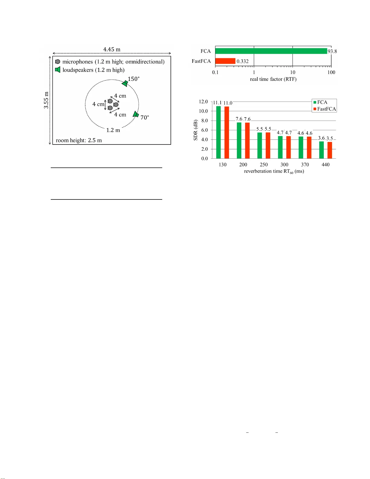
F ASTFCA: A JOINT DIA GONALIZA TION B ASED F AST ALGORITHM FOR A UDIO SOURCE SEP ARA TION USING A FULL-RANK SP A TIAL CO V ARIANCE MODEL Nobutaka Ito, Shoko Araki, T omohir o Nakatani NTT Communication Science Laboratories, NTT Corporation, Kyoto, Japan { ito.nobutaka, araki.shoko, nakatani.tom ohiro } @lab .ntt.co.jp ABSTRA CT A source separation method using a full- r ank spatial cov ariance model has been proposed by D uong et al. [“Under-de termined Rev erberant Aud io Sou rce Separation Using a Full-rank Spatial Co- v ariance Model, ” IEEE T rans. ASLP , vol. 18, no. 7, pp. 1830– 1840, Sep. 2010], which is referred to as f ull-rank spa tial covaria nce analysis (FCA) in this paper . Here we propose a fast algorithm for estimating the model parameters of the FCA, which i s named F ast- FCA , and applicable to the two-source case. Though quite effecti ve in source separation , the con ventiona l FCA has a major dra wback of expen siv e computation. Indeed, the con ventional algorithm for esti- mating the model parameters of the FCA requires frame-wise matrix in version and matrix multiplication. Therefore, the con ventional FCA may be infeasible in applications with restricted computational resources. In contrast, the proposed FastFCA byp asses matrix inv er- sion and matrix multiplication owing to j oint diagonalization based on the generalized eigen value problem. Furthermore, the FastFCA is strictl y equiv alent to the con vention al algorithm. An experiment has shown that t he FastFCA was over 250 ti mes faster than the con ventional algorithm with virtually the same source separation performance. Index T erms — Microphone arrays, source separation, joint di- agonalization, generalized eigen value problem. 1. INTRODUCTION Many audio source separation methods tak e a probabilistic approa ch, in which a probabilistic model of observed mixtures is designed and some model parameters pertinent to the sources are estimated. In such an approach, source separation performance is largely dictated by precision of the probab ilistic model. In man y conv entional mod- els, such as that in the well - known independen t component analy- sis (ICA) [1–4], the acoustic transfer characteristics of each source signal are modeled by a time-in variant steering vector . In contrast, Duong et al. [5 ] hav e proposed modeling the acoustic transfer char- acteristics of each source signal by a full-rank matrix called a spatial covar iance matrix . The latter model can properly t ake account of re- verberation , fluctuation of source locations, deviation from the ideal point-source model, etc. , whereby realizing effecti ve source separa- tion in the real world. W e call this method full-rank spatial covari- ance analysis (FCA) . A major limitation of the con ventional FCA is expensi ve compu - tation. Inde ed, t he con ventional algorithm for estimating the model parameters of t he FCA computes matrix inv erses and matrix prod- ucts frame-wise . T herefore, the con ventional FCA may be infeasible in applications with restricted computational resources. Such appli- cations may include hearing aids, distrib uted microphone arrays, and online speech enhancement. T o overco me this limitation, here we propose a fast algorithm for estimating the model p arameters of the FCA, which is nam ed F astFCA , and applicable to the two-sou rce case. The FastFCA does not require frame-wise computation of matrix in verses and matrix products, and is therefore much faster than t he conv entional algo- rithm. These frame-wise matrix operations are eliminated based on joint diagonalization of the spatial co varianc e matrices of the source signals. This is because the joint diagonalization reduces these ma- trix operations to mere scalar operations of diagonal en tries. The joint diagona lization is realized by solving a generalized eigen value problem of the spatial cov ariance matri ces of the two source signals. In the two-source case, the exact joint diagonalization is possible, and consequently the FastFCA is equiv alent to the con ventional al- gorithm, whereby causing no degradation in source separation per- formance compared to the F CA. Currently , the number of sources is limited to two in the FastFCA, and the extension to more than two sources is regarded as future work. W e follow the follo wing con ventions throughout the rest of this paper . S ignals are represented in the short-time Fourier transform (STFT) domain with the time and the frequency indices being n and f respecti vely . N denotes the number of frames, F the number of frequenc y bins up to the Nyquist frequency , N ( m , R ) the complex Gaussian distribution with mean m and cova riance matrix R , E ex- pectation, δ kl the Kr onecker delta, 0 the column zero vector of an appropriate dimension , I the i dentity matri x of an approp riate order , diag ( α 1 , α 2 , . . . , α D ) the diagonal matrix of order D with α k being its ( k , k ) entry ( k = 1 , 2 , . . . , D ), ( · ) T transposition, ( · ) H Hermitian transposition, t r ( · ) the trace, and det( · ) t he determinant. 2. FULL-RANK SP A TIAL CO V ARIANCE MA TRIX ANAL YSIS (FCA) This section briefly describes the FC A [5]. Let y ( n, f ) ∈ C I be the mixtures observed by I micro- phones wit h the i th entry corresponding to the i th microphone. Let x j ( n, f ) ∈ C I be the j th source image, where j ∈ { 1 , 2 , . . . , J } denotes the source index and J the number of sources. In this paper , we focus on the two-source case ( J = 2 ). The ob- served mixtures are mo deled as t he sum o f the source images as y ( n, f ) = x 1 ( n, f ) + x 2 ( n, f ) . W e deal with the problem of estimating x 1 ( n, f ) and x 2 ( n, f ) from y ( n, f ) . In t he FCA, the source signal x j ( n, f ) is probabilistically modeled as x j ( n, f ) ∼ N ( 0 , R j ( n, f )) , where R j ( n, f ) de- notes the cov ariance matrix of x j ( n, f ) . In t he FCA, R j ( n, f ) is parametrized as R j ( n, f ) = v j ( n, f ) S j ( f ) . (1) Here, S j ( f ) is a time-in variant Hermitian positi ve-definite (and thus full-rank) matrix called a spatial cov ariance matrix, which models the acoustic transfer characteristics of the j th source signal. v j ( n, f ) is a time-variant positiv e scalar , which models the powe r spectrum of the j th source signal. The model parame ters of the FCA, namely v j ( n, f ) and S j ( f ) , are estimated based on the maximization of the follo w i ng lik elihood: N Y n =1 F Y f =1 p ( y ( n, f )) = N Y n =1 F Y f =1 1 π I det( R 1 ( n, f ) + R 2 ( n, f )) × exp( − y ( n, f ) H ( R 1 ( n, f ) + R 2 ( n, f )) − 1 y ( n, f )) ! . (2) The likelihood (2 ) can be mon otonically increased by an expectation- maximization (E M) alg orithm [6]. The expectation st ep ( E step) updates the conditional exp ectations µ j ( n, f ) , E ( x j ( n, f ) | y ( n, f )) , (3) Φ j ( n, f ) , E ( x j ( n, f ) x j ( n, f ) H | y ( n, f )) , (4) using the current parameter estimates v ( l ) j ( n, f ) and S ( l ) j ( f ) by µ ( l +1) j ( n, f ) = v ( l ) j ( n, f ) S ( l ) j ( f ) × 2 X k =1 v ( l ) k ( n, f ) S ( l ) k ( f ) ! − 1 y ( n, f ) , (5) Φ ( l +1) j ( n, f ) = µ ( l +1) j ( n, f ) µ ( l +1) j ( n, f ) H + v ( l ) 1 ( n, f ) S ( l ) 1 ( f ) × 2 X k =1 v ( l ) k ( n, f ) S ( l ) k ( f ) ! − 1 ( v ( l ) 2 ( n, f ) S ( l ) 2 ( f )) . (6) Here, the superscript ( · ) ( l ) indicates that this variable is computed in the l th iteration, and , means definiti on. The maximization step (M step) updates the parameter estimates using Φ ( l +1) j ( n, f ) by v ( l +1) j ( n, f ) = 1 I tr ( S ( l ) j ( f ) − 1 Φ ( l +1) j ( n, f )) , (7) S ( l +1) j ( f ) = 1 N N X n =1 1 v ( l +1) j ( n, f ) Φ ( l +1) j ( n, f ) . (8) Once t he model parameters have been estimated, the source im- ages can be estimated in various ways. For example, the minimum mean square error (MMSE) estimator of x j ( n, f ) is gi ven by (5). A major drawback of the con ventional FCA is expen siv e com- putation. Indeed, the abo ve EM algorithm computes matrix inv erses and matrix products frame-wise in (5) and (6). 3. F ASTFCA This section describes the proposed FastFCA based on joint diago- nalization of t he spatial cov ariance matrices S 1 ( f ) and S 2 ( f ) . The joint diagonalization el i minates the frame-wise computation of ma- trix in verses and matrix products, becaus e the y reduce to mere scalar operations of diagonal entries for diagonal matrices. T he joint diago- nalization is realized based on the gen eralized eigen v alue problem of the matrix pair  S 1 ( f ) , S 2 ( f )  . See Appendix A for mathematical foundations of the generalized eigen value problem. Let λ ( l ) 1 ( f ) , λ ( l ) 2 ( f ) , . . . , λ ( l ) I ( f ) be the gen eralized eigen va lues of  S ( l ) 1 ( f ) , S ( l ) 2 ( f )  , and p ( l ) 1 ( f ) , p ( l ) 2 ( f ) , . . . , p ( l ) I ( f ) be general- ized eigen vectors of  S ( l ) 1 ( f ) , S ( l ) 2 ( f )  that satisfy ( S ( l ) 1 ( f ) p ( l ) i ( f ) = λ ( l ) i ( f ) S ( l ) 2 ( f ) p ( l ) i ( f ) , p ( l ) i ( f ) H S ( l ) 2 ( f ) p ( l ) k ( f ) = δ ik . (9) See Appendix A for t he existence of such λ ( l ) 1 ( f ) , λ ( l ) 2 ( f ) , . . . , λ ( l ) I ( f ) and p ( l ) 1 ( f ) , p ( l ) 2 ( f ) , . . . , p ( l ) I ( f ) . (9) can be rewritten in the fol- lo wing matrix forms: ( S ( l ) 1 ( f ) P ( l ) ( f ) = S ( l ) 2 ( f ) P ( l ) ( f ) Λ ( l ) ( f ) , P ( l ) ( f ) H S ( l ) 2 ( f ) P ( l ) ( f ) = I , (10) where P ( l ) ( f ) and Λ ( l ) ( f ) are defined by P ( l ) ( f ) ,  p ( l ) 1 ( f ) p ( l ) 2 ( f ) · · · p ( l ) I ( f )  , (11) Λ ( l ) ( f ) , diag  λ ( l ) 1 ( f ) , λ ( l ) 2 ( f ) , · · · , λ ( l ) I ( f )  . (12) From (10 ), we have P ( l ) ( f ) H S ( l ) 1 ( f ) P ( l ) ( f ) = Λ ( l ) ( f ) . (13) W e see t hat j oint diagonalization of S ( l ) 1 ( f ) and S ( l ) 2 ( f ) is realized by the transformation P ( l ) ( f ) H ( · ) P ( l ) ( f ) , where P ( l ) ( f ) is ob- tained based on the generalized eigen value prob lem of  S ( l ) 1 ( f ) , S ( l ) 2 ( f )  . No w define the follo wing v ariables that ha ve been basis- transformed by P ( l ) ( f ) : ˜ y ( l ) ( n, f ) , P ( l ) ( f ) H y ( n, f ) , (14) ˜ µ ( l +1) j ( n, f ) , P ( l ) ( f ) H µ ( l +1) j ( n, f ) , (15) ˜ Φ ( l +1) j ( n, f ) , P ( l ) ( f ) H Φ ( l +1) j ( n, f ) P ( l ) ( f ) , (16) ˜ T ( l ) j ( f ) , P ( l ) ( f ) H S ( l ) j ( f ) P ( l ) ( f ) , (17) = ( Λ ( l ) ( f ) , j = 1 , I , j = 2 , (18) ˜ S ( l +1) j ( f ) , P ( l ) ( f ) H S ( l +1) j ( f ) P ( l ) ( f ) . (19) Here, the tilde indicates the basis t ransformation. Please be careful about the difference between ( · ) ( l ) and ( · ) ( l +1) . The update rules ( 5 )–(8) are re written in terms of these new v ari- ables as i n the following, where the i ndices n and f are omitted for bre vity . ˜ µ ( l +1) j = v ( l ) j ( P ( l ) ) H S ( l ) j 2 X k =1 v ( l ) k S ( l ) k ! − 1 y ( ∵ (5) , (15)) (20) = v ( l ) j ( P ( l ) ) H S ( l ) j P ( l ) ( P ( l ) ) − 1 | {z } I 2 X k =1 v ( l ) k S ( l ) k ! − 1 × (( P ( l ) ) H ) − 1 ( P ( l ) ) H | {z } I y (21) = v ( l ) j ˜ T ( l ) j 2 X k =1 v ( l ) k ˜ T ( l ) k ! − 1 ˜ y ( l ) ( ∵ (14) , (17) ) (22) = ( v ( l ) 1 Λ ( l ) ( v ( l ) 1 Λ ( l ) + v ( l ) 2 I ) − 1 ˜ y ( l ) , j = 1 v ( l ) 2 ( v ( l ) 1 Λ ( l ) + v ( l ) 2 I ) − 1 ˜ y ( l ) , j = 2 ( ∵ (17 ) , (18)) . (23) ˜ Φ ( l +1) j = ( P ( l ) ) H µ ( l +1) j ( µ ( l +1) j ) H P ( l ) + v ( l ) 1 ( P ( l ) ) H S ( l ) 1 × 2 X k =1 v ( l ) k S ( l ) k ! − 1 ( v ( l ) 2 S ( l ) 2 ) P ( l ) ( ∵ (6) , (16 )) (24) = ( P ( l ) ) H µ ( l +1) j ( µ ( l +1) j ) H P ( l ) + v ( l ) 1 ( P ( l ) ) H S ( l ) 1 P ( l ) ( P ( l ) ) − 1 | {z } I × 2 X k =1 v ( l ) k S ( l ) k ! − 1 (( P ( l ) ) H ) − 1 ( P ( l ) ) H | {z } I ( v ( l ) 2 S ( l ) 2 ) P ( l ) (25) = ˜ µ ( l +1) j ( ˜ µ ( l +1) j ) H + v ( l ) 1 v ( l ) 2 Λ ( l ) ( v ( l ) 1 Λ ( l ) + v ( l ) 2 I ) − 1 (26) ( ∵ (15 ) , (18)) . v ( l +1) j = 1 I tr ( S ( l ) j ) − 1 (( P ( l ) ) H ) − 1 ( P ( l ) ) H | {z } I Φ ( l +1) j P ( l ) ( P ( l ) ) − 1 | {z } I ! ( ∵ (7)) (27) = 1 I tr (( ˜ T ( l ) j ) − 1 ˜ Φ ( l +1) j ) ( ∵ (16 ) , (17)) (28) =      1 I tr (( Λ ( l ) ) − 1 ˜ Φ ( l +1) 1 ) , j = 1 1 I tr ( ˜ Φ ( l +1) 2 ) , j = 2 ( ∵ (17 ) , (18)) . (29) ˜ S ( l +1) j = 1 N N X n =1 1 v ( l +1) j ˜ Φ ( l +1) j ( ∵ (8) , (16 ) , (19)) . (30) The generalized eigen vectors P ( l +1) ( f ) and the generalized eigen values Λ ( l +1) ( f ) of ( S ( l +1) 1 ( f ) , S ( l +1) 2 ( f )) hav e also to be computed to be used in the next i t eration. Note that P ( l +1) ( f ) is needed to compu te ˜ y ( l +1) ( n, f ) . One way of do ing this is to transform ˜ S ( l +1) j ( f ) back to S ( l +1) j ( f ) by S ( l +1) j ( f ) = ( P ( l ) ( f ) H ) − 1 ˜ S ( l +1) j ( f ) P ( l ) ( f ) − 1 ( ∵ (19 )) , (31) and to solv e the generalized eigenv alue problem of ( S ( l +1) 1 ( f ) , S ( l +1) 2 ( f )) . It i s possible to compute P ( l +1) ( f ) and Λ ( l +1) ( f ) more ef fi- ciently wi thout transforming ˜ S ( l +1) j ( f ) back t o S ( l +1) j ( f ) . Indeed, P ( l +1) ( f ) and Λ ( l +1) ( f ) can be computed as follo ws: P ( l +1) ( f ) = P ( l ) ( f ) Q ( l +1) ( f ) , (32) Λ ( l +1) ( f ) = Σ ( l +1) ( f ) , (33) where Q ( l +1) ( f ) and Σ ( l +1) ( f ) are the g eneralized eigen vectors and the generalized eigen values of ( ˜ S ( l +1) 1 ( f ) , ˜ S ( l +1) 2 ( f )) : Q ( l +1) ( f ) ,  q ( l +1) 1 ( f ) q ( l +1) 2 ( f ) · · · q ( l +1) I ( f )  , (34) Σ ( l +1) ( f ) , diag  σ ( l +1) 1 ( f ) , σ ( l +1) 2 ( f ) , · · · , σ ( l +1) I ( f )  . (35) Here, σ ( l +1) 1 ( f ) , σ ( l +1) 2 ( f ) , . . . , σ ( l +1) I ( f ) denote the generalized eigen values of  ˜ S ( l +1) 1 ( f ) , ˜ S ( l +1) 2 ( f )  , and q ( l +1) 1 ( f ) , q ( l +1) 2 ( f ) , . . . , q ( l +1) I ( f ) den ote generalized eigen vectors of  ˜ S ( l +1) 1 ( f ) , ˜ S ( l +1) 2 ( f )  that satisfy ( ˜ S ( l +1) 1 ( f ) q ( l +1) i ( f ) = σ ( l +1) i ( f ) ˜ S ( l +1) 2 ( f ) q ( l +1) i ( f ) , q ( l +1) i ( f ) H ˜ S ( l +1) 2 ( f ) q ( l +1) k ( f ) = δ ik . (36) Note that (36) can also be rewritten in matrix form as follows: ( ˜ S ( l +1) 1 ( f ) Q ( l +1) ( f ) = ˜ S ( l +1) 2 ( f ) Q ( l +1) ( f ) Σ ( l +1) ( f ) , Q ( l +1) ( f ) H ˜ S ( l +1) 2 ( f ) Q ( l +1) ( f ) = I . (37) T o show (32) and (33), it is sufficient t o sho w      S ( l +1) 1 ( f )( P ( l ) ( f ) Q ( l +1) ( f )) = S ( l +1) 2 ( f )( P ( l ) ( f ) Q ( l +1) ( f )) Σ ( l +1) ( f ) , ( P ( l ) ( f ) Q ( l +1) ( f )) H S ( l +1) 2 ( f )( P ( l ) ( f ) Q ( l +1) ( f )) = I . (38) This can be sho wn as follo ws: S ( l +1) 1 ( f ) P ( l ) ( f ) Q ( l +1) ( f ) = ( P ( l ) ( f ) H ) − 1 P ( l ) ( f ) H | {z } I S ( l +1) 1 ( f ) P ( l ) ( f ) Q ( l +1) ( f ) (39) = ( P ( l ) ( f ) H ) − 1 ˜ S ( l +1) 1 ( f ) Q ( l +1) ( f ) ( ∵ (19)) (40) = ( P ( l ) ( f ) H ) − 1 ˜ S ( l +1) 2 ( f ) Q ( l +1) ( f ) Σ ( l +1) ( f ) ( ∵ (37)) (41) = S ( l +1) 2 ( f ) P ( l ) ( f ) Q ( l +1) ( f ) Σ ( l +1) ( f ) ( ∵ (19)) , (42) ( P ( l ) ( f ) Q ( l +1) ( f )) H S ( l +1) 2 ( f )( P ( l ) ( f ) Q ( l +1) ( f )) = Q ( l +1) ( f ) H ˜ S ( l +1) 2 ( f ) Q ( l +1) ( f ) ( ∵ (19)) (43) = I ( ∵ (37)) . (44) As seen in (23) and (26), the proposed FastFCA does not require frame-wise matrix in version or matrix multiplication, o wing to the joint diagonalization. The additional generalized eigen v alue prob- lem and matrix multiplication in ( 32) are only required once in each frequenc y bin per iterati on instead of at all time-frequency points, and the FastFCA leads to significantly r educed computation ov erall. The algorithm is summarized as follows with L being the num- ber of iterati ons: Algorithm 1. FastFCA. 1: Set initial values v (0) j ( n, f ) , P (0) ( f ) , and Λ (0) ( f ) . Fig. 1 . Experimental setting. T ab le 1 . Experimental conditions. sampling frequenc y 16 kHz frame length 1024 (64 ms) frame shift 512 (32 ms) windo w square root of Hann number of EM iterations 10 2: for l = 0 t o L − 1 do 3: Compute ˜ y ( l ) ( n, f ) by (14). 4: Compute ˜ µ ( l +1) j ( n, f ) by ( 23 ). 5: Compute ˜ Φ ( l +1) j ( n, f ) by (26). 6: Compute v ( l +1) j ( n, f ) by (29). 7: Compute ˜ S ( l +1) j ( f ) by (30). 8: Compute Q ( l +1) ( f ) and Λ ( l +1) ( f ) by solving the general- ized eigen valu e problem of  ˜ S ( l +1) 1 ( f ) , ˜ S ( l +1) 2 ( f )  . 9: Compute P ( l +1) ( f ) by (32). 10: end for 11: Compute µ ( L ) j ( n, f ) = ( P ( L − 1) ( f ) H ) − 1 ˜ µ ( L ) j ( n, f ) , and out- put it as the estimate of the source image x j ( n, f ) . 4. SOURCE SEP ARA TION EXPERIMENT W e conducted a source separation ex periment t o compare the pro- posed FastFCA with t he con ventional FCA [5] (see Section 2). Both algorithms w ere implemented in MA TLAB (R2013a) running on an Intel i7-2600 3.4-GHz octal-core CPU. Observed mixtures were gen- erated by conv olving 8 s-long English speec h si gnals wit h room im- pulse responses measured in a room sho wn in Fig. 1 . The re verber - ation time R T 60 was 130, 200, 250, 300, 370, or 440 ms. T en trials with different speak er combinations were conducted f or each reve r- beration time. T he initi al values were computed based on esti mat- ing the spatial cova riance matrices using the time-frequenc y masks by Sawada’ s method [7]. The source images were estimated in the MMSE sense in both algorithms. Other conditions are shown in T a- ble 1. Figure 2 sho ws the real time factor (RTF) of the EM algorithm for both methods with averaging ov er all trials and all rev erberation times. Figure 3 sho ws the signal-to-distortion ratio (SDR ) [8] av er- aged over the two sources and al l trials. The input SDR was 0 dB. The FastFCA was o ver 250 times faster than the FCA with virtually the same SDR. Fig. 2 . Real time factor (R TF). Fig. 3 . Signal-to-distortion ratio (S DR). 5. CONCLUSIONS In this paper , we proposed the FastFCA , a fast algorithm for esti- mating th e FCA parameters in the tw o-source case with virtually the same SDR as the con vention al algorithm [5]. The future work includes application to denoising tasks, such as C H i ME-3 [9] and extension to more than two source signals. A. MA THEMA TICA L FOUND A TIONS OF THE GENERALIZED EIGENV ALUE PR OBLEM This appendix summarizes mathematical foundations of the gener- alized eigenv alue problem. Throughout this appendix, D denotes a positi ve integer , Φ and Ψ complex square matrices of order D , and λ a complex numbe r . λ is said to be a g eneralized eig en value of t he pair ( Φ , Ψ ) , when there exists p ∈ C D − { 0 } such that Φp = λ Ψp . When λ i s a generalized eigen value of ( Φ , Ψ ) and p ∈ C D − { 0 } satisfies Φp = λ Ψp , p is said to be a ge neralized eigen vector of ( Φ , Ψ ) correspondin g t o λ . The polynomial of λ , det( Φ − λ Ψ ) , is called t he characteris- tic polynomial of ( Φ , Ψ ) . It can be sho wn that λ is a generalized eigen value of ( Φ , Ψ ) if and only i f λ is a root of the characteristic polynomial det( Φ − λ Ψ ) . Indeed, t here exists p ∈ C D − { 0 } such that ( Φ − λ Ψ ) p = 0 if and only if the columns of Φ − λ Ψ are linearly depen dent, i.e. , det( Φ − λ Ψ ) = 0 . If Ψ is nonsingular , the fund amental theorem of algebra implies that the characteristic polynomial det( Φ − λ Ψ ) = det Ψ det( Ψ − 1 Φ − λ I ) has exactly D roots. In this sense, ( Φ , Ψ ) has exactly D gener- alized eigen valu es. Theorem 1. Sup pose Φ is Hermitian, Ψ Hermitian p ositiv e def- inite, and λ 1 , λ 2 , . . . , λ D the generalized eigen v alues of ( Φ , Ψ ) . There exist p 1 , p 2 , . . . , p D ∈ C D such that each p k is a generalized eigen vector of ( Φ , Ψ ) corresponding to λ k and p H k Ψp l = δ kl . Pr oof. Since Ψ is Hermitian positi ve definite, there exists a uni- tary matrix U and a diagonal matrix Σ with all diagonal en- tries being positive such that Ψ = UΣU H . Define a Hermitian matrix ˜ Φ by ˜ Φ = Σ − 1 2 U H ΦUΣ − 1 2 . Since det( ˜ Φ − µ I ) = det( Σ − 1 2 U H ( Φ − µ UΣU H ) UΣ − 1 2 ) = det( Ψ − 1 ) det( Φ − µ Ψ ) , λ 1 , λ 2 , . . . , λ D are the eigen values of ˜ Φ . Let q 1 , q 2 , . . . , q D ∈ C D be vectors such that each q k is an eigen vector of ˜ Φ correspond ing to λ k and q H k q l = δ kl . Define p k by p k = UΣ − 1 2 q k . It follows that Φp k = ΦUΣ − 1 2 q k = ( Σ − 1 2 U H ) − 1 Σ − 1 2 U H ΦUΣ − 1 2 q k = UΣ 1 2 ˜ Φq k = λ k UΣ 1 2 q k = λ k Ψp k . Furthermore, p H k Ψp l = q H k q l = δ kl . B. REFERENCES [1] J. -F . Cardoso, “High-order contrasts for independe nt component analysis, ” Neura l Computation , pp. 157 –192, 1999. [2] T . - W . Lee, M. Girolami, and T .J. Sejno wski, “Indepen dent com- ponent analysis using an extended infomax algorithm f or mixed subgaussian and supergaussian sources, ” Neur al Computation , pp. 417– 441, 1999. [3] A . Hyv ¨ arinen, J. Karhunen, and E. Oja, Independent Compone nt Analysis , John W i ley & Sons, New Y ork, 2001. [4] H . Sawad a, R. Mukai, S . Araki, and S . Makino, “Frequency- domain blind source separation, ” in Speech Enhancement , J. Benesty , S. Makino, and J. Chen, Eds., pp. 299– 327. S pringer , Berlin, Heidelber g, 2005. [5] N . Q. K. Duong, E. V incent, and R . Gribon val, “Under - determined re verberant audio source separation using a full-rank spatial cov ariance model, ” I EEE T rans. ASLP , vol. 18, no. 7, pp. 1830–1 840, Sep. 2010 . [6] A . P . Dempster, N.M. Laird, and D. B. Rubin, “Maximum like- lihood from incomplete data via the EM algorithm, ” Jou rnal of the Royal Statistical Society: Series B (Methodologica l) , vol. 39, no. 1, pp. 1–38, 197 7. [7] H . Sawada, S. Araki, and S. Makino , “Underdetermined con vo- lutiv e blind source separation via frequency bin-wise clustering and permutation alignment, ” I EEE T rans. ASLP , vol. 19, no. 3, pp. 516– 527, Mar . 2011. [8] E . V incent, R. Gribon val, and C. F ´ evotte, “Performance mea- surement in blind audio source separation, ” IE EE T rans. ASLP , vol. 14, no. 4, pp. 1462–14 69, Jul. 2006. [9] J. Barker , R . Marxer , E. V incent, and S. W atanabe, “The third ‘CHiME’ speech separation and recognition challenge: Dataset, task and baselines, ” in Pr oc. ASR U , Dec. 2015, pp. 504–511 .