A Purely End-to-end System for Multi-speaker Speech Recognition

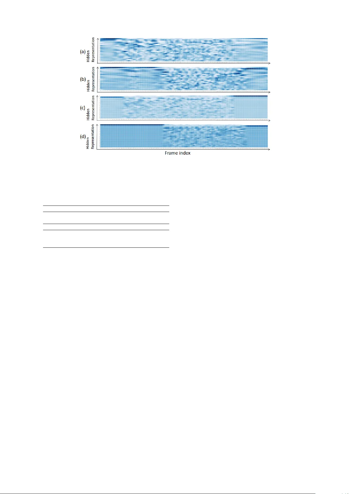
A Pur ely End-to-end System f or Multi-speaker Speech Recognition Hiroshi Seki 1,2 ∗ , T akaaki Hori 1 , Shinji W atanabe 3 , Jonathan Le Roux 1 , John R. Hershey 1 1 Mitsubishi Electric Research Laboratories (MERL) 2 T oyohashi Uni v ersity of T echnology 3 Johns Hopkins Uni versity Abstract Recently , there has been gro wing inter- est in multi-speaker speech recognition, where the utterances of multiple speak- ers are recognized from their mixture. Promising techniques hav e been proposed for this task, but earlier works ha ve re- quired additional training data such as isolated source signals or senone align- ments for effecti ve learning. In this paper , we propose a ne w sequence-to-sequence frame work to directly decode multiple la- bel sequences from a single speech se- quence by unifying source separation and speech recognition functions in an end-to- end manner . W e further propose a ne w ob- jecti ve function to impro ve the contrast be- tween the hidden vectors to a void generat- ing similar hypotheses. Experimental re- sults show that the model is directly able to learn a mapping from a speech mix- ture to multiple label sequences, achie ving 83.1% relativ e improvement compared to a model trained without the proposed ob- jecti ve. Interestingly , the results are com- parable to those produced by previous end- to-end works featuring explicit separation and recognition modules. 1 Introduction Con ventional automatic speech recognition (ASR) systems recognize a single utterance gi ven a speech signal, in a one-to-one transformation. Ho we ver , restricting the use of ASR systems to sit- uations with only a single speaker limits their ap- plicability . Recently , there has been gro wing inter - ∗ This work was done while H. Seki, Ph.D. candidate at T oyohashi University of T echnology , Japan, was an intern at MERL. est in single-channel multi-speaker speech recog- nition, which aims at generating multiple tran- scriptions from a single-channel mixture of mul- tiple speakers’ speech ( Cooke et al. , 2009 ). T o achie ve this goal, several pre vious works hav e considered a tw o-step procedure in which the mixed speech is first separated, and recognition is then performed on each separated speech sig- nal ( Hershey et al. , 2016 ; Isik et al. , 2016 ; Y u et al. , 2017 ; Chen et al. , 2017 ). Dramatic adv ances hav e recently been made in speech separation, via the deep clustering framew ork ( Hershey et al. , 2016 ; Isik et al. , 2016 ), hereafter referred to as DPCL. DPCL trains a deep neural network to map each time-frequency (T -F) unit to a high-dimensional embedding vector such that the embeddings for the T -F unit pairs dominated by the same speaker are close to each other, while those for pairs dom- inated by dif ferent speakers are farther away . The speaker assignment of each T -F unit can thus be inferred from the embeddings by simple cluster - ing algorithms, to produce masks that isolate each speaker . The original method using k-means clus- tering ( Hershey et al. , 2016 ) was extended to al- lo w end-to-end training by unfolding the cluster - ing steps using a permutation-free mask inference objecti ve ( Isik et al. , 2016 ). An alternati ve ap- proach is to perform dir ect mask infer ence using the permutation-free objectiv e function with net- works that directly estimate the labels for a fixed number of sources. Direct mask inference was first used in Hershey et al. ( 2016 ) as a baseline method, but without sho wing good performance. This ap- proach was re visited in Y u et al. ( 2017 ) and K ol- baek et al. ( 2017 ) under the name permutation- in variant training (PIT). Combination of such single-channel speaker -independent multi-speaker speech separation systems with ASR was first con- sidered in Isik et al. ( 2016 ) using a con ventional Gaussian Mixture Model/Hidden Markov Model (GMM/HMM) system. Combination with an end- to-end ASR system w as recently proposed in ( Set- tle et al. , 2018 ). Both these approaches either trained or pre-trained the source separation and ASR networks separately , making use of mixtures and their corresponding isolated clean source ref- erences. While the latter approach could in princi- ple be trained without references for the isolated speech signals, the authors found it dif ficult to train from scratch in that case. This ability can nonetheless be used when adapting a pre-trained network to ne w data without such references. In contrast with this two-stage approach, Qian et al. ( 2017 ) considered direct optimization of a deep-learning-based ASR recognizer without an explicit separation module. The network is opti- mized based on a permutation-free objectiv e de- fined using the cross-entropy between the system’ s hypotheses and reference labels. The best per- mutation between hypotheses and reference labels in terms of cross-entropy is selected and used for backpropagation. Howe ver , this method still re- quires reference labels in the form of senone align- ments, which ha ve to be obtained on the clean iso- lated sources using a single-speaker ASR system. As a result, this approach still requires the original separated sources. As a general ca v eat, generation of multiple hypotheses in such a system requires the number of speakers handled by the neural net- work architecture to be determined before train- ing. Howe ver , Qian et al. ( 2017 ) reported that the recognition of two-speaker mixtures using a model trained for three-speaker mixtures showed almost identical performance with that of a model trained on two-speak er mixtures. Therefore, it may be possible in practice to determine an upper bound on the number of speakers. Chen et al. ( 2018 ) proposed a progressi ve training procedure for a hybrid system with ex- plicit separation motiv ated by curriculum learn- ing. They also proposed self-transfer learning and multi-output sequence discriminati ve training methods for fully exploiting pairwise speech and pre venting competing hypotheses, respecti vely . In this paper , we propose to circumvent the need for the corresponding isolated speech sources when training on a set of mixtures, by using an end-to-end multi-speaker speech recognition with- out an explicit speech separation stage. In sep- aration based systems, the spectrogram is seg- mented into complementary regions according to sources, which generally ensures that different ut- terances are recognized for each speaker . W ithout this complementarity constraint, our direct multi- speaker recognition system could be susceptible to redundant recognition of the same utterance. In order to prev ent degenerate solutions in which the generated hypotheses are similar to each other , we introduce a new objecti ve function that enhances contrast between the network’ s representations of each source. W e also propose a training procedure to provide permutation in variance with lo w com- putational cost, by taking advantage of the joint CTC/attention-based encoder-decoder netw ork ar- chitecture proposed in ( Hori et al. , 2017a ). Ex- perimental results show that the proposed model is able to directly con vert an input speech mix- ture into multiple label sequences without requir- ing any explicit intermediate representations. In particular no frame-lev el training labels, such as phonetic alignments or corresponding unmixed speech, are required. W e e v aluate our model on spontaneous English and Japanese tasks and ob- tain comparable results to the DPCL based method with explicit separation ( Settle et al. , 2018 ). 2 Single-speaker end-to-end ASR 2.1 Attention-based encoder -decoder network An attention-based encoder-decoder net- work ( Bahdanau et al. , 2016 ) predicts a target label sequence Y = ( y 1 , . . . , y N ) without requir- ing intermediate representation from a T -frame sequence of D -dimensional input feature v ectors, O = ( o t ∈ R D | t = 1 , . . . , T ) , and the past label history . The probability of the n -th label y n is computed by conditioning on the past history y 1: n − 1 : p att ( Y | O ) = N Y n =1 p att ( y n | O , y 1: n − 1 ) . (1) The model is composed of two main sub-modules, an encoder network and a decoder network. The encoder network transforms the input feature v ec- tor sequence into a high-le vel representation H = ( h l ∈ R C | l = 1 , . . . , L ) . The decoder net- work emits labels based on the label history y and a context vector c calculated using an atten- tion mechanism which weights and sums the C - dimensional sequence of representation H with at- tention weight a . A hidden state e of the decoder is updated based on the previous state, the previous context v ector , and the emitted label. This mecha- nism is summarized as follo ws: H = Encoder( O ) , (2) y n ∼ Decoder( c n , y n − 1 ) , (3) c n , a n = A tten tion( a n − 1 , e n , H ) , (4) e n = Up date( e n − 1 , c n − 1 , y n − 1 ) . (5) At inference time, the previously emitted labels are used. At training time, they are replaced by the reference label sequence R = ( r 1 , . . . , r N ) in a teacher -forcing fashion, leading to conditional probability p att ( Y R | O ) , where Y R denotes the out- put label sequence variable in this condition. The detailed definitions of Atten tion and Up date are described in Section A of the supplementary mate- rial. The encoder and decoder networks are trained to maximize the conditional probability of the ref- erence label sequence R using backpropagation: L att = Loss att ( Y R , R ) , − log p att ( Y R = R | O ) , (6) where Loss att is the cross-entropy loss function. 2.2 Joint CTC/attention-based encoder -decoder network The joint CTC/attention approach ( Kim et al. , 2017 ; Hori et al. , 2017a ), uses the connection- ist temporal classification (CTC) objective func- tion ( Grav es et al. , 2006 ) as an auxiliary task to train the network. CTC formulates the condi- tional probability by introducing a framewise la- bel sequence Z consisting of a label set U and an additional blank symbol defined as Z = { z l ∈ U ∪ { ’blank’ }| l = 1 , · · · , L } : p ctc ( Y | O ) = X Z L Y l =1 p ( z l | z l − 1 , Y ) p ( z l | O ) , (7) where p ( z l | z l − 1 , Y ) represents monotonic align- ment constraints in CTC and p ( z l | O ) is the frame- le vel label probability computed by p ( z l | O ) = Softmax(Linear( h l )) , (8) where h l is the hidden representation generated by an encoder network, here taken to be the en- coder of the attention-based encoder-decoder net- work defined in Eq. ( 2 ), and Linear( · ) is the final linear layer of the CTC to match the number of labels. Unlike the attention model, the forward- backward algorithm of CTC enforces monotonic alignment between the input speech and the out- put label sequences during training and decod- ing. W e adopt the joint CTC/attention-based encoder-decoder network as the monotonic align- ment helps the separation and extraction of high- le vel representation. The CTC loss is calculated as: L ctc = Loss ctc ( Y , R ) , − log p ctc ( Y = R | O ) . (9) The CTC loss and the attention-based encoder- decoder loss are combined with an interpolation weight λ ∈ [0 , 1] : L mtl = λ L ctc + (1 − λ ) L att . (10) Both CTC and encoder-decoder networks are also used in the inference step. The final hypothe- sis is a sequence that maximizes a weighted condi- tional probability of CTC in Eq. ( 7 ) and attention- based encoder decoder network in Eq. ( 1 ): ˆ Y = arg max Y  γ log p ctc ( Y | O ) + (1 − γ ) log p att ( Y | O )  , (11) where γ ∈ [0 , 1] is an interpolation weight. 3 Multi-speaker end-to-end ASR 3.1 Permutation-fr ee training In situations where the correspondence between the outputs of an algorithm and the references is an arbitrary permutation, neural network training faces a permutation pr oblem . This problem was first addressed by deep clustering ( Hershey et al. , 2016 ), which circumv ented it in the case of source separation by comparing the relationships between pairs of network outputs to those between pairs of labels. As a baseline for deep clustering, Hershe y et al. ( 2016 ) also proposed another approach to ad- dress the permutation problem, based on an ob- jecti ve which considers all permutations of refer- ences when computing the error with the network estimates. This objectiv e was later used in Isik et al. ( 2016 ) and Y u et al. ( 2017 ). In the latter , it was referred to as permutation-in variant training. This permutation-free training scheme extends the usual one-to-one mapping of outputs and la- bels for backpropagation to one-to-many by se- lecting the proper permutation of hypotheses and references, thus allowing the network to generate multiple independent hypotheses from a single- channel speech mixture. When a speech mixture contains speech uttered by S speakers simulta- neously , the network generates S label sequence v ariables Y s = ( y s 1 , . . . , y s N s ) with N s labels from the T -frame sequence of D -dimensional input fea- ture vectors, O = ( o t ∈ R D | t = 1 , . . . , T ) : Y s ∼ g s ( O ) , s = 1 , . . . , S, (12) where the transformations g s are implemented as neural networks which typically share some com- ponents with each other . In the training stage, all possible permutations of the S sequences R s = ( r s 1 , . . . , r s N 0 s ) of N 0 s reference labels are consid- ered (considering permutations on the hypotheses would be equiv alent), and the one leading to min- imum loss is adopted for backpropagation. Let P denote the set of permutations on { 1 , . . . , S } . The final loss L is defined as L = min π ∈P S X s =1 Loss( Y s , R π ( s ) ) , (13) where π ( s ) is the s -th element of a permutation π . For example, for two speakers, P includes two permutations (1 , 2) and (2 , 1 ), and the loss is de- fined as: L = min(Loss( Y 1 , R 1 ) + Loss( Y 2 , R 2 ) , Loss( Y 1 , R 2 ) + Loss( Y 2 , R 1 )) . (14) Figure 1 shows an overvie w of the proposed end-to-end multi-speaker ASR system. In the fol- lo wing Section 3.2 , we describe an extension of encoder network for the generation of multiple hidden representations. W e further introduce a permutation assignment mechanism for reducing the computation cost in Section 3.3 , and an ad- ditional loss function L K L for promoting the dif- ference between hidden representations in Sec- tion 3.4 . 3.2 End-to-end permutation-free training T o make the netw ork output multiple hypotheses, we consider a stacked architecture that combines both shared and unshared (or specific) neural net- work modules. The particular architecture we con- sider in this paper splits the encoder network into three stages: the first stage, also referred to as mixture encoder , processes the input mixture and Figure 1: End-to-end multi-speaker speech recog- nition. W e propose to use the permutation-free training for CTC and attention loss functions Loss ctc and Loss att , respecti vely . outputs an intermediate feature sequence H ; that sequence is then processed by S independent en- coder sub-networks which do not share param- eters, also referred to as speaker-dif ferentiating (SD) encoders, leading to S feature sequences H s ; at the last stage, each feature sequence H s is inde- pendently processed by the same network, also re- ferred to as recognition encoder , leading to S final high-le vel representations G s . Let u ∈ { 1 . . . , S } denote an output index (cor - responding to the transcription of the speech by one of the speakers), and v ∈ { 1 . . . , S } de- note a reference index. Denoting by Encoder Mix the mixture encoder , Enco der u SD the u -th speak er - dif ferentiating encoder , and Enco der Rec the recognition encoder , an input sequence O corre- sponding to an input mixture can be processed by the encoder network as follo ws: H = Encoder Mix ( O ) , (15) H u = Enco der u SD (H) , (16) G u = Enco der Rec ( H u ) . (17) The motiv ation for designing such an architecture can be explained as follows, follo wing analogies with the architectures in ( Isik et al. , 2016 ) and ( Settle et al. , 2018 ) where separation and recog- nition are performed explicitly in separate steps: the first stage in Eq. ( 15 ) corresponds to a speech separation module which creates embedding v ec- tors that can be used to distinguish between the multiple sources; the speaker-dif ferentiating sec- ond stage in Eq. ( 16 ) uses the first stage’ s output to disentangle each speaker’ s speech content from the mixture, and prepare it for recognition; the fi- nal stage in Eq. ( 17 ) corresponds to an acoustic model that encodes the single-speaker speech for final decoding. The decoder network computes the conditional probabilities for each speaker from the S outputs of the encoder network. In general, the decoder network uses the reference label R as a history to generate the attention weights during training, in a teacher -forcing fashion. Howe ver , in the abov e permutation-free training scheme, the reference label to be attributed to a particular output is not determined until the loss function is computed, so we here need to run the attention decoder for all reference labels. W e thus need to consider the con- ditional probability of the decoder output variable Y u,v for each output G u of the encoder network under the assumption that the reference label for that output is R v : p att ( Y u,v | O ) = Y n p att ( y u,v n | O , y u,v 1: n − 1 ) , (18) c u,v n , a u,v n = A tten tion( a u,v n − 1 , e u,v n , G u ) , (19) e u,v n = Up date( e u,v n − 1 , c u,v n − 1 , r v n − 1 ) , (20) y u,v n ∼ Decoder( c u,v n , r v n − 1 ) . (21) The final loss is then calculated by considering all permutations of the reference labels as follo ws: L att = min π ∈P X s Loss att ( Y s,π ( s ) , R π ( s ) ) . (22) 3.3 Reduction of permutation cost In order to reduce the computational cost, we fix ed the permutation of the reference labels based on the minimization of the CTC loss alone, and used the same permutation for the attention mechanism as well. This is an advantage of using a joint CTC/attention based end-to-end speech recogni- tion. Permutation is performed only for the CTC loss by assuming synchronous output where the permutation is decided by the output of CTC: ˆ π = arg min π ∈P X s Loss ctc ( Y s , R π ( s ) ) , (23) where Y u is the output sequence v ariable corre- sponding to encoder output G u . Attention-based decoding is then performed on the same hidden representations G u , using teacher forcing with the labels determined by the permutation ˆ π that mini- mizes the CTC loss: p att ( Y u, ˆ π ( u ) | O ) = Y n p att ( y u, ˆ π ( u ) n | O , y u, ˆ π ( u ) 1: n − 1 ) , c u, ˆ π ( u ) n , a u, ˆ π ( u ) n = A tten tion( a u, ˆ π ( u ) n − 1 , e u, ˆ π ( u ) n , G u ) , e u, ˆ π ( u ) n = Up date( e u, ˆ π ( u ) n − 1 , c u, ˆ π ( u ) n − 1 , r ˆ π ( u ) n − 1 ) , y u, ˆ π ( u ) n ∼ Decoder( c u, ˆ π ( u ) n , r ˆ π ( u ) n − 1 ) . This corresponds to the “permutation assignment” in Fig. 1 . In contrast with Eq. ( 18 ), we only need to run the attention-based decoding once for each output G u of the encoder network. The final loss is defined as the sum of two objective functions with interpolation λ : L mtl = λ L ctc + (1 − λ ) L att , (24) L ctc = X s Loss ctc ( Y s , R ˆ π ( s ) ) , (25) L att = X s Loss att ( Y s, ˆ π ( s ) , R ˆ π ( s ) ) . (26) At inference time, because both CTC and attention-based decoding are performed on the same encoder output G u and should thus pertain to the same speaker , their scores can be incorpo- rated as follo ws: ˆ Y u = arg max Y u  γ log p ctc ( Y u | G u ) + (1 − γ ) log p att ( Y u | G u )  , (27) where p ctc ( Y u | G u ) and p att ( Y u | G u ) are obtained with the same encoder output G u . 3.4 Promoting separation of hidden vectors A single decoder network is used to output mul- tiple label sequences by independently decoding the multiple hidden vectors generated by the en- coder network. In order for the decoder to gener- ate multiple different label sequences the encoder needs to generate sufficiently differentiated hidden vector sequences for each speaker . W e propose to encourage this contrast among hidden vectors by introducing in the objectiv e function a new term based on the ne gati ve symmetric K ullback-Leibler (KL) div ergence. In the particular case of two- speaker mixtures, we consider the following ad- ditional loss function: L KL = − η X l  KL( ¯ G 1 ( l ) || ¯ G 2 ( l )) + KL( ¯ G 2 ( l ) || ¯ G 1 ( l ))  , (28) where η is a small constant value, and ¯ G u = (softmax( G u ( l )) | l = 1 , . . . , L ) is ob- tained from the hidden vector sequence G u at the output of the recognition encoder Enco der Rec as in Fig. 1 by applying an additional frame-wise softmax operation in order to obtain a quantity amenable to a probability distribution. 3.5 Split of hidden vector for multiple hypotheses Since the network maps acoustic features to la- bel sequences directly , we consider various archi- tectures to perform implicit separation and recog- nition effecti vely . As a baseline system, we use the concatenation of a V GG-moti v ated CNN net- work ( Simonyan and Zisserman , 2014 ) (referred to as VGG) and a bi-directional long short-term memory (BLSTM) network as the encoder net- work. For the splitting point in the hidden vector computation, we consider two architectural varia- tions as follo ws: • Split by BLSTM: The hidden vector is split at the le vel of the BLSTM network. 1) the VGG network generates a single hidden vector H ; 2) H is fed into S independent BLSTMs whose parameters are not shared with each other; 3) the output of each independent BLSTM H u , u = 1 , . . . , S, is further separately fed into a unique BLSTM, the same for all outputs. Each step corresponds to Eqs. ( 15 ), ( 16 ), and ( 17 ). • Split by V GG: The hidden vector is split at the le vel of the VGG network. The number of filters at the last con volution layer is multiplied by the number of mixtures S in order to split the out- put into S hidden vectors (as in Eq. ( 16 )). The layers prior to the last VGG layer correspond to the network in Eq. ( 15 ), while the subsequent BLSTM layers implement the network in ( 17 ). 4 Experiments 4.1 Experimental setup W e used English and Japanese speech corpora, WSJ (W all street journal) ( Consortium , 1994 ; T able 1: Duration (hours) of unmixed and mixed corpora. The mixed corpora are generated by Al- gorithm 1 in Section B of the supplementary ma- terial, using the training, de velopment, and ev alu- ation set respecti vely . T R A I N D E V . E V A L W S J ( U N M I X E D ) 8 1 . 5 1 . 1 0 . 7 W S J ( M I X E D ) 9 8 . 5 1 . 3 0 . 8 C S J ( U N M I X E D ) 5 8 3 . 8 6 . 6 5 . 2 C S J ( M I X E D ) 8 2 6 . 9 9 . 1 7 . 5 Garofalo et al. , 2007 ) and CSJ (Corpus of spon- taneous Japanese) ( Maeka wa , 2003 ). T o show the ef fecti veness of the proposed models, we gener- ated mixed speech signals from these corpora to simulate single-channel ov erlapped multi-speaker recording, and ev aluated the recognition perfor- mance using the mixed speech data. For WSJ, we used WSJ1 SI284 for training, De v93 for de velop- ment, and Eval92 for ev aluation. For CSJ, we fol- lo wed the Kaldi recipe ( Moriya et al. , 2015 ) and used the full set of academic and simulated pre- sentations for training, and the standard test sets 1, 2, and 3 for e v aluation. W e created ne w corpora by mixing two utter- ances with different speakers sampled from exist- ing corpora. The detailed algorithm is presented in Section B of the supplementary material. The sampled pairs of two utterances are mix ed at vari- ous signal-to-noise ratios (SNR) between 0 dB and 5 dB with a random starting point for the overlap. Duration of original unmixed and generated mix ed corpora are summarized in T able 1 . 4.1.1 Network architecture As input feature, we used 80-dimensional log Mel filterbank coef ficients with pitch features and their delta and delta delta features ( 83 × 3 = 249 - dimension) extracted using Kaldi tools ( Povey et al. , 2011 ). The input feature is normalized to zero mean and unit variance. As a baseline sys- tem, we used a stack of a 6-layer VGG network and a 7-layer BLSTM as the encoder network. Each BLSTM layer has 320 cells in each direc- tion, and is follo wed by a linear projection layer with 320 units to combine the forward and back- ward LSTM outputs. The decoder network has an 1-layer LSTM with 320 cells. As described in Section 3.5 , we adopted two types of encoder ar- chitectures for multi-speaker speech recognition. The network architectures are summarized in T a- ble 2 . The split-by-VGG network had speaker dif ferentiating encoders with a con volution layer T able 2: Network architectures for the en- coder network. The number of layers is indi- cated in parentheses. Enco der Mix , Enco der u SD , and Encoder Rec correspond to Eqs. ( 15 ), ( 16 ), and ( 17 ). S P L I T B Y Enco der Mix Enco der u SD Enco der Rec N O V G G ( 6 ) — B L S T M ( 7 ) V G G V G G ( 4 ) V G G ( 2 ) B L S T M ( 7 ) B L S T M V G G ( 6 ) B L S T M ( 2 ) B L S T M ( 5 ) (and the follo wing maxpooling layer). The split- by-BLSTM network had speaker dif ferentiating encoders with two BLSTM layers. The architec- tures were adjusted to hav e the same number of layers. W e used characters as output labels. The number of characters for WSJ w as set to 49 includ- ing alphabets and special tokens (e.g., characters for space and unkno wn). The number of charac- ters for CSJ was set to 3,315 including Japanese Kanji/Hiragana/Katakana characters and special tokens. 4.1.2 Optimization The network was initialized randomly from uni- form distribution in the range -0.1 to 0.1. W e used the AdaDelta algorithm ( Zeiler , 2012 ) with gradient clipping ( P ascanu et al. , 2013 ) for opti- mization. W e initialized the AdaDelta hyperpa- rameters as ρ = 0 . 95 and  = 1 − 8 .  is de- cayed by half when the loss on the de velopment set degrades. The networks were implemented with Chainer ( T okui et al. , 2015 ) and ChainerMN ( Ak- iba et al. , 2017 ). The optimization of the networks was done by synchronous data parallelism with 4 GPUs for WSJ and 8 GPUs for CSJ. The networks were first trained on single- speaker speech, and then retrained with mixed speech. When training on unmixed speech, only one side of the network only (with a single speaker dif ferentiating encoder) is optimized to output the label sequence of the single speaker . Note that only character labels are used, and there is no need for clean source reference corresponding to the mixed speech. When mo ving to mixed speech, the other speaker-dif ferentiating encoders are ini- tialized using the already trained one by copying the parameters with random perturbation, w 0 = w × (1 + Uniform( − 0 . 1 , 0 . 1)) for each param- eter w . The interpolation v alue λ for the multiple objecti ves in Eqs. ( 10 ) and ( 24 ) was set to 0 . 1 for WSJ and to 0 . 5 for CSJ. Lastly , the model is re- trained with the additional negati ve KL di ver gence loss in Eq. ( 28 ) with η = 0 . 1 . T able 3: Ev aluation of unmixed speech without multi-speaker training. T A S K A V G . W S J 2 . 6 C S J 7 . 8 4.1.3 Decoding In the inference stage, we combined a pre- trained RNNLM (recurrent neural network lan- guage model) in parallel with the CTC and de- coder network. Their label probabilities were lin- early combined in the log domain during beam search to find the most likely hypothesis. For the WSJ task, we used both character and word le vel RNNLMs ( Hori et al. , 2017b ), where the charac- ter model had a 1-layer LSTM with 800 cells and an output layer for 49 characters. The word model had a 1-layer LSTM with 1000 cells and an output layer for 20,000 words, i.e., the vocab ulary size was 20,000. Both models were trained with the WSJ te xt corpus. For the CSJ task, we used a char - acter level RNNLM ( Hori et al. , 2017c ), which had a 1-layer LSTM with 1000 cells and an out- put layer for 3,315 characters. The model parame- ters were trained with the transcript of the training set in CSJ. W e added language model probabilities with an interpolation factor of 0.6 for character- le vel RNNLM and 1.2 for w ord-le vel RNNLM. The beam width for decoding was set to 20 in all the experiments. Interpolation γ in Eqs. ( 11 ) and ( 27 ) was set to 0.4 for WSJ and 0.5 for CSJ. 4.2 Results 4.2.1 Evaluation of unmixed speech First, we examined the performance of the base- line joint CTC/attention-based encoder -decoder network with the original unmixed speech data. T able 3 sho ws the character error rates (CERs), where the baseline model sho wed 2.6% on WSJ and 7.8% on CSJ. Since the model w as trained and e v aluated with unmixed speech data, these CERs are considered lo wer bounds for the CERs in the succeeding experiments with mix ed speech data. 4.2.2 Evaluation of mixed speech T able 4 shows the CERs of the generated mixed speech from the WSJ corpus. The first col- umn indicates the position of split as mentioned in Section 3.5 . The second, third and forth columns indicate CERs of the high ener gy speaker ( H I G H E . S P K .), the low energy speaker ( L OW E . S P K .), and the average ( A V G .), respectiv ely . The baseline model has very high CERs because T able 4: CER (%) of mixed speech for WSJ. S P L I T H I G H E . S P K . L OW E . S P K . A V G . N O ( B A SE L I N E ) 8 6 . 4 7 9 . 5 8 3 . 0 V G G 1 7 . 4 1 5 . 6 1 6 . 5 B L S T M 1 4 . 6 13.3 1 4 . 0 + K L L O S S 14.0 13.3 13.7 T able 5: CER (%) of mixed speech for CSJ. S P L I T H I G H E . S P K . L OW E . S P K . A V G . N O ( B A SE L I N E ) 9 3 . 3 9 2 . 1 9 2 . 7 B L S T M 11.0 18.8 14.9 it was trained as a single-speaker speech recog- nizer without permutation-free training, and it can only output one hypothesis for each mixed speech. In this case, the CERs were calculated by du- plicating the generated hypothesis and comparing the duplicated hypotheses with the correspond- ing references. The proposed models, i.e., split- by-VGG and split-by-BLSTM networks, obtained significantly lo wer CERs than the baseline CERs, the split-by-BLSTM model in particular achie ving 14.0% CER. This is an 83.1% relati ve reduction from the baseline model. The CER w as further re- duced to 13.7% by retraining the split-by-BLSTM model with the negati ve KL loss, a 2.1% rela- ti ve reduction from the network without retrain- ing. This result implies that the proposed negati ve KL loss provides better separation by activ ely im- proving the contrast between the hidden vectors of each speaker . Examples of recognition results are sho wn in Section C of the supplementary ma- terial. Finally , we profiled the computation time for the permutations based on the decoder network and on CTC. Permutation based on CTC was 16.3 times faster than that based on the decoder net- work, in terms of the time required to determine the best match permutation giv en the encoder net- work’ s output in Eq. ( 17 ). T able 5 shows the CERs for the mix ed speech from the CSJ corpus. Similarly to the WSJ ex- periments, our proposed model significantly re- duced the CER from the baseline, where the av er- age CER was 14.9% and the reduction ratio from the baseline was 83.9%. 4.2.3 V isualization of hidden vectors W e show a visualization of the encoder networks outputs in Fig. 2 to illustrate the ef fect of the ne g- ati ve KL loss function. Principal component anal- ysis (PCA) was applied to the hidden v ectors on the vertical axis. Figures 2 (a) and 2 (b) sho w the hidden vectors generated by the split-by-BLSTM model without the negati ve KL di ver gence loss for an example mixture of two speakers. W e can observe different acti v ation patterns showing that the hidden vectors were successfully separated to the individual utterances in the mix ed speech, al- though some acti vity from one speaker can be seen as leaking into the other . Figures 2 (c) and 2 (d) sho w the hidden vectors generated after retrain- ing with the negati ve KL di ver gence loss. W e can more clearly observe the dif ferent patterns and boundaries of acti vation and deactiv ation of hid- den vectors. The negati ve KL loss appears to re g- ularize the separation process, and e ven seems to help in finding the end-points of the speech. 4.2.4 Comparison with earlier work W e first compared the recognition performance with a hybrid (non end-to-end) system including DPCL-based speech separation and a Kaldi-based ASR system. It was ev aluated under the same e v aluation data and metric as in ( Isik et al. , 2016 ) based on the WSJ corpus. Howe ver , there are dif- ferences in the size of training data and the op- tions in decoding step. Therefore, it is not a fully matched condition. Results are sho wn in T able 6 . The word error rate (WER) reported in ( Isik et al. , 2016 ) is 30.8%, which was obtained with jointly trained DPCL and second-stage speech enhance- ment networks. The proposed end-to-end ASR gi ves an 8.4% relati ve reduction in WER ev en though our model does not require any explicit frame-le vel labels such as phonetic alignment, or clean signal reference, and does not use a phonetic lexicon for training. Although this is an unfair comparison, our purely end-to-end system outper- formed a hybrid system for multi-speaker speech recognition. Next, we compared our method with an end- to-end explicit separation and recognition net- work ( Settle et al. , 2018 ). W e retrained our model pre viously trained on our WSJ-based corpus using the training data generated by Settle et al. ( 2018 ), because the direct optimization from scratch on their data caused poor recognition performance due to data size. Other experimental conditions are shared with the earlier work. Interestingly , our method showed comparable performance to the end-to-end explicit separation and recognition network, without having to pre-train using clean signal training references. It remains to be seen if this parity of performance holds in other tasks and conditions. Figure 2: V isualization of the two hidden v ector sequences at the output of the split-by-BLSTM encoder on a two-speak er mixture. (a,b): Generated by the model without the negati ve KL loss. (c,d): Generated by the model with the negati ve KL loss. T able 6: Comparison with con ventional ap- proaches M E T H OD W E R ( % ) D P C L + A S R ( I S I K E T A L . , 2 0 1 6 ) 3 0 . 8 Proposed end-to-end ASR 28.2 M E T H OD C E R ( % ) E N D - TO - E N D D P C L + A S R ( C H A R L M ) ( S E T TL E E T A L . , 2 0 1 8 ) 13.2 Proposed end-to-end ASR (char LM) 1 4 . 0 5 Related work Se veral pre vious works have considered an ex- plicit two-step procedure ( Hershey et al. , 2016 ; Isik et al. , 2016 ; Y u et al. , 2017 ; Chen et al. , 2017 , 2018 ). In contrast with our work which uses a sin- gle objecti ve function for ASR, the y introduced an objecti ve function to guide the separation of mix ed speech. Qian et al. ( 2017 ) trained a multi-speaker speech recognizer using permutation-free training without explicit objecti ve function for separation. In contrast with our work which uses an end-to- end architecture, their objecti ve function relies on a senone posterior probability obtained by align- ing unmix ed speech and te xt using a model trained as a recognizer for single-speaker speech. Com- pared with ( Qian et al. , 2017 ), our method di- rectly maps a speech mixture to multiple character sequences and eliminates the need for the corre- sponding isolated speech sources for training. 6 Conclusions In this paper , we proposed an end-to-end multi- speaker speech recognizer based on permutation- free training and a new objecti ve function pro- moting the separation of hidden vectors in order to generate multiple hypotheses. In an encoder- decoder network frame work, teacher forcing at the decoder network under multiple refer - ences increases computational cost if implemented nai vely . W e a voided this problem by employing a joint CTC/attention-based encoder-decoder net- work. Experimental results sho wed that the model is able to directly con vert an input speech mixture into multiple label sequences under the end-to-end frame work without the need for any e xplicit inter - mediate representation including phonetic align- ment information or pairwise unmixed speech. W e also compared our model with a method based on explicit separation using deep clustering, and sho wed comparable result. Future work includes data collection and ev aluation in a real world scenario since the data used in our experiments are simulated mixed speech, which is already ex- tremely challenging but still leaves some acous- tic aspects, such as Lombard ef fects and real room impulse responses, that need to be alle viated for further performance improvement. In addition, further study is required in terms of increasing the number of speakers that can be simultane- ously recognized, and further comparison with the separation-based approach. References T akuya Akiba, Keisuke Fukuda, and Shuji Suzuki. 2017. ChainerMN: Scalable Distributed Deep Learning Framew ork. In Proceedings of W ork- shop on ML Systems in The Thirty-first Annual Con- fer ence on Neural Information Pr ocessing Systems (NIPS) . Dzmitry Bahdanau, Jan Chorowski, Dmitriy Serdyuk, Philemon Brakel, and Y oshua Bengio. 2016. End- to-end attention-based large vocabulary speech recognition. In IEEE International Conference on Acoustics, Speech and Signal Pr ocessing (ICASSP) , pages 4945–4949. Zhehuai Chen, Jasha Droppo, Jinyu Li, and W ayne Xiong. 2018. Progressiv e joint modeling in unsu- pervised single-channel overlapped speech recogni- tion. IEEE/ACM T ransactions on Audio, Speech, and Language Pr ocessing , 26(1):184–196. Zhuo Chen, Y i Luo, and Nima Mesgarani. 2017. Deep attractor network for single-microphone speaker separation. In IEEE International Conference on Acoustics, Speech and Signal Pr ocessing (ICASSP) , pages 246–250. Jan K Chorowski, Dzmitry Bahdanau, Dmitriy Serdyuk, Kyunghyun Cho, and Y oshua Bengio. 2015. Attention-based models for speech recogni- tion. In Advances in Neural Information Pr ocessing Systems (NIPS) , pages 577–585. Linguistic Data Consortium. 1994. CSR-II (wsj1) complete. Linguistic Data Consortium, Philadel- phia , LDC94S13A. Martin Cooke, John R Hershey , and Stev en J Ren- nie. 2009. Monaural speech separation and recog- nition challenge. Computer Speech and Languag e , 24(1):1–15. John Garofalo, David Graff, Doug P aul, and Da vid P al- lett. 2007. CSR-I (wsj0) complete. Linguistic Data Consortium, Philadelphia , LDC93S6A. Alex Graves, Santiago Fern ´ andez, Faustino Gomez, and J ¨ urgen Schmidhuber . 2006. Connectionist temporal classification: labelling unsegmented se- quence data with recurrent neural networks. In International Confer ence on Machine learning (ICML) , pages 369–376. John R Hershe y , Zhuo Chen, Jonathan Le Roux, and Shinji W atanabe. 2016. Deep clustering: Discrim- inativ e embeddings for segmentation and separa- tion. In IEEE International Confer ence on Acous- tics, Speech and Signal Pr ocessing (ICASSP) , pages 31–35. T akaaki Hori, Shinji W atanabe, and John R Hershey . 2017a. Joint CTC/attention decoding for end-to-end speech recognition. In Pr oceedings of the 55th An- nual Meeting of the Association for Computational Linguistics (ACL): Human Language T echnologies: long papers . T akaaki Hori, Shinji W atanabe, and John R Hershey . 2017b. Multi-lev el language modeling and decod- ing for open vocab ulary end-to-end speech recog- nition. In IEEE W orkshop on Automatic Speech Recognition and Understanding (ASR U) . T akaaki Hori, Shinji W atanabe, Y u Zhang, and Chan W illiam. 2017c. Advances in joint CTC-Attention based end-to-end speech recognition with a deep CNN encoder and RNN-LM. In Inter speech , pages 949–953. Y usuf Isik, Jonathan Le Roux, Zhuo Chen, Shinji W atanabe, and John R. Hershey . 2016. Single- channel multi-speaker separation using deep cluster- ing. In Pr oc. Interspeech , pages 545–549. Suyoun Kim, T akaaki Hori, and Shinji W atanabe. 2017. Joint CTC-attention based end-to-end speech recognition using multi-task learning. In IEEE In- ternational Confer ence on Acoustics, Speech and Signal Pr ocessing (ICASSP) , pages 4835–4839. Morten Kolbæk, Dong Y u, Zheng-Hua T an, and Jes- per Jensen. 2017. Multitalker speech separation with utterance-level permutation in variant training of deep recurrent neural networks. IEEE/A CM T ransactions on A udio, Speech, and Language Pr o- cessing , 25(10):1901–1913. Kikuo Maekaw a. 2003. Corpus of Spontaneous Japanese: Its design and ev aluation. In ISCA & IEEE W orkshop on Spontaneous Speech Pr ocessing and Recognition . T akafumi Moriya, T akahiro Shinozaki, and Shinji W atanabe. 2015. Kaldi recipe for Japanese sponta- neous speech recognition and its ev aluation. In Au- tumn Meeting of ASJ , 3-Q-7. Razvan Pascanu, T omas Mikolov , and Y oshua Bengio. 2013. On the dif ficulty of training recurrent neu- ral networks. International Confer ence on Machine Learning (ICML) , pages 1310–1318. Daniel Povey , Arnab Ghoshal, Gilles Boulianne, Lukas Burget, Ondrej Glembek, Nagendra Goel, Mirko Hannemann, Petr Motlicek, Y anmin Qian, Petr Schwarz, Jan Silovsk y , Geor g Stemmer, and Karel V esely . 2011. The kaldi speech recognition toolkit. In IEEE W orkshop on A utomatic Speec h Recogni- tion and Understanding (ASR U) . Y anmin Qian, Xuankai Chang, and Dong Y u. 2017. Single-channel multi-talker speech recognition with permutation in v ariant training. arXiv pr eprint arXiv:1707.06527 . Shane Settle, Jonathan Le Roux, T akaaki Hori, Shinji W atanabe, and John R. Hershey . 2018. End-to-end multi-speaker speech recognition. In IEEE Interna- tional Confer ence on Acoustics, Speech and Signal Pr ocessing (ICASSP) , pages 4819–4823. Karen Simonyan and Andre w Zisserman. 2014. V ery deep conv olutional networks for lar ge-scale image recognition. arXiv pr eprint arXiv:1409.1556 . Seiya T okui, Kenta Oono, Shohei Hido, and Justin Clayton. 2015. Chainer: a next-generation open source frame work for deep learning. In Pr oceedings of W orkshop on Machine Learning Systems (Learn- ingSys) in NIPS . Dong Y u, Morten Kolbk, Zheng-Hua T an, and Jesper Jensen. 2017. Permutation in variant training of deep models for speaker-independent multi-talker speech separation. In IEEE International Conference on Acoustics, Speech and Signal Pr ocessing (ICASSP) , pages 241–245. Matthew D Zeiler . 2012. ADADEL T A: an adap- tiv e learning rate method. arXiv pr eprint arXiv:1212.5701 . A Architectur e of the encoder -decoder network In this section, we describe the details of the baseline encoder-decoder network which is fur- ther e xtended for permutation-free training. The encoder network consists of a VGG network and bi-directional long short-term memory (BLSTM) layers. The VGG network has the follo wing 6- layer CNN architecture at the bottom of the en- coder network: Con volution (# in = 3, # out = 64, filter = 3 × 3) Con volution (# in = 64, # out = 64, filter = 3 × 3) MaxPooling (patch = 2 × 2, stride = 2 × 2) Con volution (# in = 64, # out = 128, filter = 3 × 3) Con volution (# in=128, # out=128, filter=3 × 3) MaxPooling (patch = 2 × 2, stride = 2 × 2) The first 3 channels are static, delta, and delta delta features. Multiple BLSTM layers with projection layer Lin( · ) are stacked after the VGG network. W e defined one BLSTM layer as the concatena- tion of a forward LSTM − − − − − − → LSTM( · ) and a backward LSTM ← − − − − − − LSTM( · ) : − → H = − − − − → LSTM( · ) (29) ← − H = ← − − − − LSTM( · ) (30) H = [Lin( − → H ); Lin( ← − H )] , (31) When the VGG network and the multiple BLSTM layers are represented as V GG( · ) and BLSTM( · ) , the encoder network in Eq. ( 2 ) maps the input fea- ture vector O to internal representation H as fol- lo ws: H = Encoder( O ) = BLSTM(V GG( O )) (32) The decoder network sequentially generates the n -th label y n by taking the context v ector c n and the label history y 1: n − 1 : y n ∼ Decoder( c n , y n − 1 ) . (33) The context vector is calculated in an location based attention mechanism ( Choro wski et al. , 2015 ) which weights and sums the C -dimensional sequence of representation H = ( h l ∈ R C | l = 1 , . . . , L ) with attention weight a n,l : c n = A tten tion( a n − 1 , e n , H ) , (34) , L X l =1 a n,l h l . (35) Algorithm 1 Generation of multi speaker speech dataset n reuse ⇐ maximum number of times same ut- terance can be used. U ⇐ utterance set of the corpora. C k ⇐ n reuse for each utterance U k ∈ U f or U k ∈ U do P ( U k ) = C k / P l C l end f or f or U i in U do Sample utterance U j from P ( U ) while ensur - ing speakers of U i and U j are dif ferent. Mix utterances U i and U j if C j > 0 then C j = C j − 1 f or U k ⇐ U do P ( U k ) = C k / P l C l end f or end if end f or The location based attention mechanism defines the weights a n,l as follo ws: a n,l = exp( αk n,l ) P L l =1 exp( αk n,l ) , (36) k n,l = w T tanh( V E e n − 1 + V H h l + V F f n,l + b ) , (37) f n = F ∗ a n − 1 , (38) where w , V E , V H , V F , b, F are tunable parame- ters, α is a constant value called in verse tempera- ture, and ∗ is the con volution operation. W e used 10 conv olution filters of width 200 , and set α to 2. The introduction of f n makes the attention mech- anism take into account the previous alignment in- formation. The hidden state e is updated recur- si vely by an updating LSTM function: e n = Up date( e n − 1 , c n − 1 , y n − 1 ) , (39) , LSTM( Lin( e n − 1 ) + Lin( c n − 1 ) + Em b( y n − 1 )) , (40) where Em b( · ) is an embedding function. B Generation of mixed speech Each utterance of the corpus is mixed with a randomly selected utterance with the probability , P ( U k ) , that moderates over -selection of specific utterances. P ( U k ) is calculated in the first for-loop as a uniform probability . All utterances are used as T able 7: Examples of recognition results. Errors are emphasized as capital letter . “ ” is a space character , and a special token “*” is inserted to pad deletion errors. (1) Model w/ permutation-fr ee training (CER of HYP1: 12.8%, HYP2: 0.9%) HYP1: t h e s h u t t l e * * * I S I N t h e f i r s t t H E l i f E o * f s i n c e t h e n i n e t e e n e i g h t y s i x c h a l l e n g e r e x p l o s i o n REF1 : t h e s h u t t l e W O U L D B E t h e f i r s t t * O l i f T o F f s i n c e t h e n i n e t e e n e i g h t y s i x c h a l l e n g e r e x p l o s i o n HYP2: t h e e x p a n d e d r e c a l l w a s d i s c l o s e d a t a m e e t i n g w i t h n . r . c . o f f i c i a l s a t a n a g e n c y o f f i c e o u t s i d e c h i c a g o REF2 : t h e e x p a n d e d r e c a l l w a s d i s c l o s e d a t a m e e t i n g w i t h n . r . c . o f f i c i a l s a t a n a g e n c y o f f i c e o u t s i d e c h i c a g o (2) Model w/ permutation-fr ee training (CER of HYP1: 91.7%, HYP2: 38.9%) HYP1: I T W A S L a s t r * A I S e * D * I N J U N E N I N E t E e N e * I G h T Y f I V e T O * T H I R T Y REF1: * * * * * * * * a s t * r O N O M e R S S A Y T H A T * * * * t H e * e A R T h ’ S f A T e I S S E A L E D HYP2: * * * * a N D * * s t * r O N G e R S S A Y T H A T * * * * t H e * e * A R t H f A T e I S t o f o r t y f i v e d o l l a r s f r o m t h i r t y f i v e d o l l a r s REF2: I T W a * S L A s t r A I S e * D * I N J U N E N I N E t E e N e I G H t Y f I V e * * * t o f o r t y f i v e d o l l a r s f r o m t h i r t y f i v e d o l l a r s one side of the mixture, and another side is sam- pled from the distribution P ( U k ) in the second for- loop. The selected pairs of utterances are mixed at v arious signal-to-noise ratios (SNR) between 0 dB and 5 dB. W e randomized the starting point of the ov erlap by padding the shorter utterance with si- lence whose duration is sampled from the uniform distribution within the length difference between the two utterances. Therefore, the duration of the mixed utterance is equal to that of the longer utter - ance among the unmixed speech. After the gen- eration of the mix ed speech, the count of selected utterances C j is decremented to prevent of over - selection. All counts C are set to n reuse , and we used n reuse = 3 . C Examples of recognition results and error analysis T able 7 shows examples of recognition result. The first example (1) is one which accounts for a large portion of the ev aluation set. The SNR of the HYP1 is -1.55 db and that of HYP2 is 1.55 dB. The network generates multiple hypotheses with a few substitution and deletion errors, but without any o verlapped and sw apped words. The second example (2) is one which leads to performance re- duction. W e can see that the network makes errors when there is a large difference in length between the tw o sequences. The word “thirty” of HYP2 is injected in HYP1, and there are deletion errors in HYP2. W e added a negati ve KL di ver gence loss to ease such kind of errors. Howe ver , there is further room to reduce error by making unshared modules more cooperati ve.