Restoring a smooth function from its noisy integrals

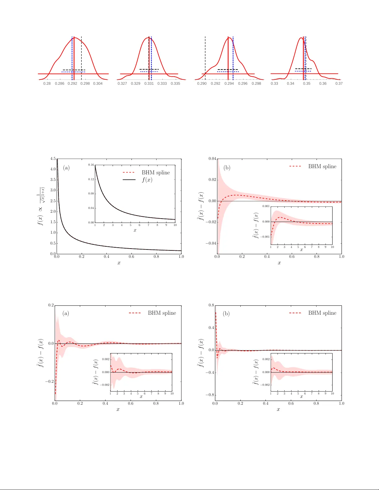
Restoring a smo oth function from its noisy in tegrals Olga Goulk o Dep artment of Physics, University of Massachusetts, A mherst, MA 01003, USA and Pr esent addr ess: R aymond and Beverly Sackler Scho ol of Chemistry and School of Physics and Astr onomy, T el Aviv University, T el Aviv 6997801, Isr ael Nik olay Prok of ’ev Dep artment of Physics, University of Massachusetts, Amherst, MA 01003, USA and National R ese ar ch Center “Kur chatov Institute,” 123182 Mosc ow, Russia Boris Svistunov Dep artment of Physics, University of Massachusetts, Amherst, MA 01003, USA National Rese ar ch Center “Kur chatov Institute,” 123182 Mosc ow, Russia and Wilczek Quantum Center, Scho ol of Physics and Astr onomy and T. D. L e e Institute, Shanghai Jiao T ong University, Shanghai 200240, China (Dated: May 14, 2018) Numerical (and exp erimen tal) data analysis often requires the restoration of a smo oth function from a set of sampled integrals ov er finite bins. W e presen t the bin hierarch y metho d that efficiently computes the maximally smooth function from the sampled integrals using essentially all the infor- mation con tained in the data. W e p erform extensiv e tests with different classes of functions and lev els of data qualit y , including Monte Carlo data suffering from a sev ere sign problem and physical data for the Green’s function of the F r¨ ohlic h p olaron. P A CS n umbers: 02.60.-x, 02.70.-c, 07.05.Rm, 87.57.np I. INTR ODUCTION Sampling is at the heart of many Monte Carlo com- putations and exp erimental measuremen ts. Data p oin ts are generated or measured and w e ev entually wan t to restore the underlying smo oth probabilit y densit y dis- tribution f ( x ) b ehind them. Man y density estimation proto cols for lists of statistical data exist, 1–3 but for large-scale Mon te Carlo calculations storing the individ- ual data p oin ts would require p entab ytes of memory and lead to a substantial slowing down of the sim ulation. More importantly , the individual data p oints are not needed, provided that we know that f ( x ) is structure- less below a certain scale. Hence, without losing an y es- sen tial information, w e can collect in tegrals of f ( x ) o ver finite-size bins. The problem then is ho w to extract all the information from these integrals without systematic bias, augmenting it with our a priori kno wledge of the smo othness of the function. In this paper, we propose a simple and efficient solu- tion, whic h we call the bin hierarch y metho d (BHM). 4 W e note that the problem is closely related to the prob- lem of numerical analytic con tinuation under consisten t constrain ts, 5 but with a crucial simplification. Unlik e for the numerical restoration of sp ectral functions, we do not ha ve to accoun t for p ossible sharp features, suc h as δ - function p eaks or kinks, which cannot b e resolved within the sampled error bars. Assuming that f ( x ) is smo oth, w e are allow ed to parametrize its optimal appro ximation ˜ f ( x ) as a p olynomial spline (or a spline with a general functional ansatz). The protocol of constructing ˜ f ( x ) has some similarities with the smo othing spline approach. 6 Ho wev er, there is a fundamental difference in the data structure. Rather than fitting to appro ximate function v alues on a given set of p oints, we fit the spline directly to the sampled in tegrals. The central requiremen t is that ˜ f ( x ) m ust b e consisten t not only with the sampled in tegrals ov er the elemen tary histogram bins, but also with the integrals o ver an y combination of these. In tegrals o ver large bins are kno wn with higher precision than those o ver smaller bins, since the former con tain more data points. Hence, accurately reco vering a large in tegral is a priorit y o v er re- co vering a smaller one. In particular, bins below a certain scale con tain noise rather than information about f ( x ), and thus can b e safely omitted in the fitting. W e formal- ize this idea b y introducing a hierarc h y of bins with one bin o ver the en tire domain of f ( x ) on the top level, and doubling the num b er of bins on each subsequent lev el. The go o dness of fit is ev aluated on each level n sepa- rately , with χ 2 n / ˜ n as the measure, where ˜ n is the num b er of bins on the giv en hierarch y lev el. Out of all p ossible approximations ˜ f ( x ) consisten t with the sampled integrals we select the one with the least features, i.e. the one with the least fitting parameters. This is ac hiev ed by fitting a spline of order m (t ypically m = 3) with the minimal num b er of knots that yields an acceptable fit. The n umber and the p ositions of the knots are determined automatically b y the fitting algo- rithm. Kno wn b oundary conditions on f ( x ) can also b e accoun ted for. If desired, additional optimization terms, for instance for the jump in the highest spline deriv ative, can b e included in to the fitting procedure, with iterative impro vemen t in the spirit of the metho d of consistent 2 constrain ts. 7 The pap er is organized as follows. In Sec. I I, we re- view alternative metho ds to construct ˜ f ( x ) and argue that the BHM is superior in accuracy , efficiency , and sim- plicit y . The details of the BHM are presented in Sec. I I I. In Sec. IV, we presen t several tests of the BHM. W e con- clude in Sec. V. I I. REVIEW OF AL TERNA TIVE METHODS A. Naiv e histograms The most straigh tforw ard w ay to approximate a distri- bution f ( x ) is the histogram: 1–3 divide the domain into sev eral bins and count how many times the sampled v al- ues of x , whic h were generated with probabilities giv en b y f ( x ), fall into each of the bins. F or each generated x ∈ bin i , the counter c i for the bin i is increased b y one. The distribution is then appro ximated by ˜ f ( x ) = X i c i N ∆ i Π i ( x ) , (1) where N is the total num b er of sampled p oints, ∆ i is the width of the bin i , and Π i ( x ) is the boxcar function, whic h is one if x ∈ bin i and zero otherwise. In what fol- lo ws, w e refer to this metho d as “naiv e histogramming”— to emphasize the contrast with the BHM that also in- v olves histogramming as a part of the proto col. The end result of the naiv e histogram metho d is a staircase func- tion, which is not smo oth. This drawbac k can b e amelio- rated by taking c i / ( N ∆ i ) as the v alue of ˜ f ( x ) at the bin cen ters and fitting a smo othing spline to the data with their statistical error bars. 6 A more imp ortant issue is that the naive histogram metho d suffers from an inher- en t compromise b etw een the resolution of features and statistical noise. Sufficien tly narrow bins are necessary to resolve f ( x ) without in tro ducing a significan t system- atic bias, while reducing the size of the bins increases the noise in the sampled coun ters. B. Basis pro jection method A generalization of the naiv e histogram metho d—the basis pro jection metho d—can significantly reduce this dra wback. This method is based on a generalized F ourier series expansion of f ( x ). F or each bin i , we choose a ba- sis { e ( j ) i ( x ) } of m i real-v alued functions with e ( j ) i ( x ) = 0 if x / ∈ bin i that satisfy the orthonormalit y condition h e ( j ) i | e ( j 0 ) i i ≡ Z bin i w i ( x ) e ( j ) i ( x ) e ( j 0 ) i ( x ) dx = δ j j 0 . (2) The non-negative weigh t function w i ( x ) of the inner pro duct should be chosen such that all in tegrals are con- v ergent. If no divergences are presen t w i ( x ) can b e set to unit y . The basis and weigh t functions ma y b e differen t for each bin, and can be defined also for bins of infinite size. In general, the basis functions can b e c hosen to re- flect the properties of f ( x ) that are known in adv ance, for instance kno wn divergences or asymptotic b eha vior. Otherwise, in the ma jorit y of the cases, shifted Legendre p olynomials are a reasonable c hoice. With the basis pro jection metho d, in eac h bin i w e k eep track of sev eral counters c ( j ) i estimating the m i gen- eralized F ourier co efficients h e ( j ) i | f i . Sp ecifically , eac h time w e generate x ∈ bin i w e add the v alue w i ( x ) e ( j ) i ( x ) (rather than one) to eac h of the c ( j ) i coun ters. The func- tion ˜ f ( x ) is then given b y ˜ f ( x ) = X i m i X j =1 c ( j ) i N e ( j ) i ( x ) . (3) Note that Eq. (1) is a sp ecial case of the ab o ve form ula with m i = 1, w i ( x ) = 1, and e (1) i ( x ) = Π i ( x ) / √ ∆ i . It can be easily seen that this pro cedure corresp onds to the b est p ossible represen tation of f ( x ) in terms of orthogonal basis functions on each bin i , since minimizing Z bin i w i ( x )( f ( x ) − ˜ f ( x )) 2 dx = = Z bin i w i ( x )   f ( x ) − m i X j =1 c ( j ) i N e ( j ) i ( x )   2 dx (4) with respect to the c ( j ) i implies Z bin i w i ( x ) e ( j ) i ( x )   f ( x ) − m i X j 0 =1 c ( j 0 ) i N e ( j 0 ) i ( x )   dx = 0 , (5) and consequen tly c ( j ) i / N = h e ( j ) i | f i . Using basis pro jections we collect more information in eac h sampling step than with the naive histogram, since some information ab out the p osition of x inside the bin is preserv ed. Therefore few er bins are necessary to resolve the function. The bin widths and basis sizes m i can b e c hosen in a wa y that the systematic error is negligible compared to the statistical error, without a substan tial increase in the statistical noise of the ˜ f ( x ) v alues. While the basis pro jection method is a significan t im- pro vemen t o ver the naive histogram, it still has several disadv antages. The binning and the basis functions m ust b e chosen at the b eginning of the sampling pro cess and cannot be altered retrosp ectively . Basis pro jections can also be computationally exp ensiv e, especially for a large basis, or a basis built of complicated functions. Moreov er, the sampled pro jections generally exhibit large jumps at the bin b oundaries b ecause the basis functions ma y b e un b ounded. As b efore, w e can eliminate these jumps by taking the v alues of ˜ f ( x ) at several points inside each bin 3 and then constructing a smoothing spline. This pro ce- dure, how ever, in volv es an unnecessary loss of informa- tion. Rather than reducing the fit to specific individual p oin ts, it is suggestive to fit a spline to the sampled inte- grals h e ( j ) i | f i directly , resulting in smaller errors. In addi- tion, we can extract more exhaustive information ab out f ( x ) by using ov erlapping bins of differen t size that co ver a range of relev ant scales of the function. This is ac hieved b y the BHM describ ed in Sec. I II. C. Rew eighting Rew eighting is a Monte Carlo-sp ecific tec hnique that allo ws one to con v ert the statistics generated for a given v ariable x to statistics for other v alues of this v ariable. 8,9 This is ac hieved in the following wa y . Prior to sampling, w e choose a fixed set of p oints x i and asso ciate a bin with each of the x i . The bins can b e large and o v erlap- ping. Whenever the random v ariable x falls into the bin i associated with the p oin t x i , w e up date the x i coun ter b y the reweigh ted v alue vp ( x i ) /p ( x ). Here v is the v alue that w ould hav e b een sampled without rew eighting, and p ( x i ) /p ( x ) is the ratio of the probability w eights at x i and x , where p ( x ) is the probability distribution used to sample the physical function f ( x ). This can b e seen as a deterministic “update” from the generated point x to the fixed p oint x i . F or sufficien tly large bins, sev eral coun ters ma y be up dated simultaneously for eac h gener- ated x . The reweigh ting technique provides an unbiased estimator for the v alue f ( x i ) at any fixed x i . The reweigh ting metho d is very efficient in the case when one is interested in a single special v alue of a certain con tinuous v ariable. A c haracteristic example is the sam- pling of the single-particle density matrix from the statis- tics for the Green’s function by reweigh ting the latter to the imaginary-time v alue τ = − 0. In all other cases, rew eighting is computationally expensive compared to the gain in accuracy . It also requires a case-sp ecific imple- men tation that assumes knowledge of the analytical form of the rew eigh ting factors. T o b e maximally efficien t, one has to adjust the size of bin i for each x i of interest. The bin size m ust b e optimized in such a wa y that, on the one hand, it is large enough to ensure sufficiently large statistics, and on the other hand small enough that the rew eighting factors remain of the order of unit y (to av oid n umerous v anishingly small contributions that consume sim ulation time). Bins that are too large can also result in a strong increase in the auto correlation time, since rew eighting from a rare even t to a frequen t one implies a large p ( x i ) /p ( x ) ratio, whic h will result in o ccasional anomalously large contributions to the sampled coun ters. Moreo ver, to pro duce a smooth outcome, the rew eighting proto col requires an appropriately dense mesh of p oints with strongly ov erlapping bins, which is computationally exp ensiv e since a large num b er of counters needs to b e up dated for eac h generated x . F or a contin uous set of function v alues, a smo othing spline needs to b e fitted at additional computational cost, comparable to the cost of the BHM fit describ ed in Sec. II I. I II. BIN HIERAR CHY METHOD The BHM restores smooth distributions in a universal, un biased, and efficient manner. The metho d satisfies the follo wing requiremen ts: • All the information con tained in the sampled data should b e used to fit the distribution: the accuracy should b e essen tially the same as if w e had stored the full list of the generated v alues of x . This is ac hieved by introducing a hierarch y of ov erlapping histogram bins of different size, where large bins giv e precise estimates of the broad features of the distribution, while s mall bins resolv e its fine struc- ture once enough data has accumulated. Note that w e assume that the sampled distribution is struc- tureless below a certain scale, and hence there al- w ays exists a binning that is sufficien tly fine to re- solv e all of its features. • The resulting function should b e exactly smo oth, meaning that the function and all its deriv atives up to a given order must ha ve no jumps. This is ac hieved by fitting a p olynomial (or generalized) spline. • Out of all smooth functions consistent with the sampled data within its error bars, the selected re- sult should ha ve the least features (p eaks, oscilla- tions, etc.). This is achiev ed by c ho osing the spline with the minimal n umber of free parameters that fits the data. • The sampling pro cess and the restoration of the smo oth function should b e computationally and memory efficient. In particular, they should b e more efficien t than the basis pro jection metho d. • The algorithm should w ork well regardless of the qualit y and the n umber of sampled data. As more data are collected and statistics improv es, so should the fitted distribution without needing an y external adjustmen ts. • The algorithm should b e highly automated. No h uman input or con trol should b e necessary other than a limited c hoice of initial parameters. In par- ticular, the metho d should b e applicable to all rea- sonably o ccurring functions and should require no adjustmen t for differen t classes of functions. Belo w w e describe the setup in detail. A. Sampling stage W e divide the domain into 2 K non-o verlapping elemen- tary bins that do not need to b e of equal width. Because 4 in the end we form com binations of sev eral bins, the ele- men tary bins ma y b e arbitrarily small. Bins with to o few data p oin ts are automatically excluded from the analy- sis. As the n umber of sampled points increases, bins of smaller size will b ecome usable. The num b er of elemen- tary bins is thus limited only b y memory . The K → ∞ limit w ould formally corresp ond to k eeping the full list of the generated v alues of x . In practice, the distributions of interest are structureless beyond a certain scale that sets a natural limit on the required elemen tary bin width. W e generate v alues of x according to a probabil- it y distribution given by | f ( x ) | (imp ortance sampling) and sample the v alue v = sign[ f ( x )] in the elementary bin i that contains x . W e can also include additional w eighting co efficien ts into the sampled v alues. F or each bin we store the num b er of sampled v alues in the bin, N i , as well as the av erage ¯ v i and the scaled v ariance M 2 ( v i ) = ( N i − 1)V ar( v i ) of the sampled v alues o v er the bin. W e obtain the s ampled in tegral I i o ver eac h elemen- tary bin via I i = ¯ v i N i / N , where N is the total n umber of sampled points. The v ariance of the sampled in tegral is calculated via V ar( I i ) = M 2 ( I i ) N − 1 (6) M 2 ( I i ) = M 2 ( v i ) + ¯ v 2 i N i ( N − N i ) N (7) and its error is giv en by δ I i = p V ar( I i ) / N . B. Bin hierarch y After sampling has finished, w e construct com binations of elementary bins. These make up a hierarc hy with 2 n bins at each level n ∈ { 0 , . . . , K } . At the top level we ha ve one large bin containing the en tire in tegral; on the next level we hav e tw o bins con taining the in tegrals o v er half of the in terv al each, etc. The fit is constructed to minimize K X n =0 χ 2 n 2 n = χ 2 0 1 + χ 2 1 2 + . . . + χ 2 K 2 K , (8) where χ 2 n is the goo dness of the fit considering only the bins on the level n . Note that the construction of the bin hierarc hy happ ens in the p ost pro cessing. During the sampling stage, only the v alues N i , ¯ v i and M 2 ( v i ) in the elemen tary bins (corresp onding to the hierarch y level K ) need to b e collected and stored. W e tested several mo difications of this setup, which pro duced consisten t results. Including more than 2 n bins on eac h lev el b y using ov erlapping bins of equal size w as found to bring no significan t impro vemen t. Likewise, us- ing weigh ts other than 1 / 2 n for χ 2 n did not impro ve the result. In general, finer bins at higher levels do not sub- stan tially con tribute to the form of the fit, as their error bars are large and the shape of the distribution is usually already determined by the lo wer-lev el in tegrals. But they are still included into the fitting pro cedure (provided that they contain enough data p oin ts for statistics) to resolve p oten tial fine structures of the distribution. F or example, a perio dically oscillating function lik e the sine can ha v e zero a verage ov er large parts of the domain, while b eing nonzero on a finer scale. The structure of suc h a function will b e resolved from the integrals ov er small bins if they con tain enough data. Due to the 1 / 2 n w eight factors, the small bins cannot ov erp o wer the large bin con tributions. Note that while for minimization we use the sum o ver all lev els, to decide whether a fit is accepted w e c heck the go odness of the fit at ev ery level separately . A fit is ac- cepted only if e ach of the χ 2 n / ˜ n is approximately 1, within a given num b er T of standard deviations σ = p 2 / ˜ n ( ˜ n ≤ 2 n is the num b er of bins on level n which con- tain sufficient data to be used for fitting). The fit accep- tance threshold T is an external input parameter, typi- cally T = 2. Low er v alues of the threshold are lik ely to result in the failure to pro duce an acceptable fit. Instead of a fixed v alue, a range of T can also b e sp ecified, for example betw een tw o and four. If there is no acceptable fit at the low est threshold v alue, it is gradually increased un til either the maxim um is reached or an acceptable fit is found. F or a large n um b er of hierarc h y lev els, the sta- tistical probabilit y for a level to exceed a 2 σ threshold on χ 2 n / ˜ n b ecomes non-negligible, even if the ov erall fit is go od. Sp ecifying a threshold range allows one to attempt fits with low er threshold v alues, without risking a failed fit. C. P olynomial fit The sampled in tegrals are fitted to a spline. In what follo ws w e discuss p olynomial (typically , cubic) splines, but a generalization to other functions is straigh tforward. Here we briefly review the theory of fitting a single poly- nomial p ( x ) = P m k =0 a k x k , before we turn to the full spline in the next section. There exists a lot of standard softw are for fitting a set of p oints to a function. Here we wan t to match the p oly- nomial to a set of integrals, which requires a sligh t adjust- men t. The deriv ation follo ws the steps of general linear least squares fitting. 10 The b est polynomial fit minimizes χ 2 = X i I i − I ( p ) i δ I i ! 2 , (9) where I ( p ) i is the in tegral of the polynomial ov er the bin i . F or simplicity we omit the sum o ver bin levels and the corresp onding w eighting factors in this section, but the generalization is straightforw ard. Let us lab el the b oundaries of bin i b y ¯ x i and ¯ x i +1 . The in tegral of the p olynomial ov er the bin equals Z ¯ x i +1 ¯ x i p ( x ) dx = m X k =0 a k k + 1 ( ¯ x k +1 i +1 − ¯ x k +1 i ) ≡ m X k =0 a k X ik 5 (10) and Eq. (9) b ecomes χ 2 = X i I i δ I i − m X k =0 a k X ik δ I i ! 2 ≡ X i b i − X k A ik a k ! 2 = | A · a − b | 2 . (11) The v ector b con tains the sampled in tegrals divided by the error bar (its length equals the num ber of bins ˜ n ), the vector a of length m + 1 contains the free parameters of the polynomial, and the ˜ n × ( m + 1) design matrix A is defined by A ik = X ik /δ I i . The design matrix has more ro ws than columns since there must b e more data points than fit parameters. W e find the vector a that minimizes | A · a − b | 2 using singular v alue decomp osition of the design matrix. 10 The error on the fitted p olynomial at a given p oin t x is obtained from the co v ariance matrix C j k = Co v( a j , a k ) via δ p ( x ) = v u u t m X i,j =0 C ij x i + j . (12) D. Spline A t eac h knot b etw een t w o spline pieces, the v alues of the corresp onding p olynomials and their deriv atives up to order ( m − 1) are equal. This giv es m constraints at eac h knot. Since eac h polynomial has m + 1 co efficients, the total n umber of free parameters is n p + m , where n p is the num b er of spline pieces. The extra m parameters arise since there is one more p olynomial piece than knots. Kno wn b oundary conditions, if any , further reduce the n umber of free parameters. The algorithm determines the p ositions of the knots using the following pro cedure. Begin by attempting to fit one p olynomial on the whole in terv al. If this fit is not acceptable, split the in terv al into tw o equal parts and attempt fitting a t wo-piece spline. If this fit is not acceptable either, c heck the go o dness of the fit on each in terv al separately . In terv als where the fit is not accept- able hav e to b e split in the next iteration, while all other in terv als remain unc hanged. Rep eat this pro cedure until either an acceptable fit is found, or the interv als can no longer b e split. W e require that the set of equations for eac h spline piece be ov erdetermined, i.e. that the n umber of bins inside eac h in terv al is larger than m + 1. This sets the limit on the maximal num b er of spline pieces. T o chec k the go o dness of the fit on an individual in- terv al, w e compute the v alues of χ 2 n / ˜ n , where χ 2 n is ev al- uated only on bins of level n that are fully inside the giv en interv al (and that contain enough statistical data), and ˜ n is the num b er of such bins. Larger bins that reach o ver sev eral interv als cannot be used for this c heck, but they are used to chec k the go odness of the ov erall fit. In all test cases, if the polynomials on the individual in- terv als passed the go odness-of-fit test, the ov erall spline ev aluated o ver the entire domain passed also. Note that as before, the c hecks on the individual in terv als are per- formed for each hierarc hy lev el separately . If more than half of the level n bins inside a given in terv al do not co n- tain enough data, the chec k for this in terv al terminates without proceeding to subsequen t lev els. E. Constraining jumps in the highest deriv ative An additional constraint on the jumps in the m th deriv ative of the spline can be imp osed on the final fit, if desired. Deriv atives up to order m − 1 are matched at the spline knots, while all deriv atives of order greater than m are zero. The piecewise constant m th deriv ative, whic h is proportional to the v alue of the parameter a ( j ) m on each interv al j , is the only one that exhibits jumps at the knots. Imp osing an additional constraint that aims to minimize these jumps ensures a con tin uous ev olution of the fitted spline as a function of the n um b er of sam- pled points N . The num b er of spline pieces for the best fit generally increases with growing N , as b etter statistics p ermits a better resolution of the sampled function. Ad- ditional interv al divisions are triggered at certain discrete v alues of N , namely when one of the χ 2 n v alues on the af- fected in terv al crosses the goo dness-of-fit threshold. This creates an additional jump in the m th deriv ative at the p osition of the new knot. This jump can be closed with only a small sacrifice in χ 2 n since the previous spline with one few er knot w as almost acceptable. In this sense, the additional constrain t on the jump acts as a comp ensation mec hanism for a p oten tially to o vigorous interv al split- ting. In most cases, constraining the jump has almost no effect of the fit. The constrain t term has the form λ n p n p − 1 X j =1 λ j a ( j +1) m − a ( j ) m ¯ a ( j +1) m − ¯ a ( j ) m ! 2 , (13) where ¯ a ( j ) m are the p olynomial parameters of the opti- mal fit without the constrain t and the w eights λ and λ j con trol the strength of the constraint. After comput- ing the optimal spline through minimization of Eq. (8), a new spline fit is attempted on the same interv al di- vision, this time b y minimizing the sum of (8) and the constrain t (13). The lo cal w eights λ j are determined b y the go o dness of the original fit (without constraint) on the interv als j − 1, j , j + 1 and j + 2, whic h are adjacent or next-to-adjacent to the respective knot. Sp ecifically , w e determine (on each hierarc hy level of each of these in terv als) the difference b etw een the maximally accept- able χ 2 n / ˜ n = 1 + T p 2 / ˜ n and the actual χ 2 n / ˜ n . W e take λ j to be the minimum of all these differences. This en- sures that the constrain t does not affect spline in terv als 6 where already the original fit was barely acceptable. The global weigh t λ is iteratively adjusted to the maximal v alue that is still compatible with the imp osed thresh- old on the χ 2 n / ˜ n . Additional iterations can b e p erformed b y replacing the ¯ a ( j ) m with the v alues calculated with the constrain t. F. Errors on the spline co efficients An estimate on the spline co efficient errors can b e ob- tained from Eq. (12) for each spline piece. This equation is accurate for parametric fits to a set of statistically in- dep enden t normally distributed data p oin ts. This is not the case for the BHM, due to the o v erlapping bins and the unconv entional χ 2 -minimization proto col. Because of this, one cannot attach Gaussian standard deviation probabilities to error bars. A robust wa y of defining the error at a given p oint x is to lo ok at the histogram of ˜ f ( x ) v alues ov er a large set of indep endent runs with the same sample size N . The smallest interv al around the histogram mean that con tains 68 . 27% of the ˜ f ( x ) v alues corresp onds to the robust estimate for tw o standard er- rors ( ± 1 σ ). This is the most rigorous, alb eit impractical, w ay of defining the error under these circumstances. A suitable alternativ e proto col should yield errors that are close to the robust v alue. W e p erformed extensiv e tests of sev eral error estima- tion proto cols by comparing them to the robust estimate for differen t types of distribution f ( x ). These tests con- firmed that Eq. (12) provides a go od error estimate in most cases. In some cases the error w as found to b e o verestimated by a factor of ab out tw o compared to the robust error. This o ccurred in particular at the domain b oundaries and for BHM splines with a large num b er of knots. A concrete example is presented in Sec. IV C. The error w as nev er observ ed to be to o small and hence Eq. (12) gives a con venien t and efficient wa y to obtain a conserv ative error estimate on the BHM fit. A tigh ter error estimate can b e obtained using b ootstrap 11 with the follo wing proto col. Pro duce an ar- ra y of M histograms eac h of which contains a fraction N / M of the N sampled data points, so that each p oint is sampled in exactly one of the histograms. Generate ˜ M ≥ M b o otstrap histograms by taking ˜ M random linear combinations (with positive in teger coefficients) of the M histograms. Each of these b o otstrapped his- tograms then contains N sampled points, but with p os- sible rep etitions. Run the BHM fit on eac h of the bo ot- strap histograms fixing the p ositions of the knots to b e the same as for the BHM fit of the regular histogram (the sum of all bo otstrap histograms with unit weigh t) and without ev aluating the go o dness of fit. The error on the spline co efficients is then determined from the statis- tics on the b o otstrapp ed histogram fits in the usual w ay . The b o otstrap error was found to b e very close to the robust error estimate in all our tests. This sc heme uses more resources, esp ecially memory , since M & 100 his- tograms need to b e stored instead of one. The increase in computational time is less significant, since p erforming fits with fixed knot positions is v ery fast. Another error estimation proto col is based on the anal - ysis of the evolution of the BHM fit as a function of sam- ple size N . F or this, the BHM spline is pro duced and sa ved perio dically in in terv als of ∆ sampling steps. The idea is that the fit results ˜ f ( x ) will approach the exact v alue with the disp ersion σ ∝ 1 / √ N . The interv al size ∆ m ust be large enough to guaran tee that the con tributions A k from differen t in terv als are statistically independent, allo wing one to inv oke the central limit theorem: ˜ f k = 1 k k X i =1 A i ⇒ A k = k ˜ f k − ( k − 1) ˜ f k − 1 . (14) The disp ersion of ˜ f k can then b e obtained from the dis- p ersion σ ∗ of the indep endent A k via σ 2 k = σ 2 ∗ /k . An additional cutoff k ≥ k 0 should also b e introduced to re- duce the effect of the initial p ortion of the statistics that can b e strongly affected by transien t pro cesses. A simple consistency criterion is that there should b e a range of ∆ and k 0 suc h that σ ∗ is essentially indep endent of b oth parameters. Our tests sho w ed that the errors calculated with this method are almost indistinguishable from the ones obtained with b o otstrap, and hence also agree with the robust error. This method is somewhat slo wer, since the full BHM fit needs to b e ev aluated rep eatedly , and requires a sufficiently large N . On the other hand, the A k sequence pro vides explicit insigh t in to the statistics of the data and can help to identify statistical fluctuations. G. Sign problem Mon te Carlo sampling often suffers from a sign prob- lem, when p ositive and negativ e terms o ccur with almost equal frequency in the sampling pro cess. Before a suffi- cien t amount of data has been collected, the error may th us substantially exceed the absolute v alue of the sam- pled integrals. The same applies to the error of the fitted spline. Fits where the noise substan tially exceeds the sig- nal are unsuitable for further data analysis. T o iden tify this problem, the algorithm chec ks—at all bin levels— whether the sampled data are consisten t with zero before the start of the fitting process. The data is deemed c er- tainly inc onsistent with zero only if at least one of the follo wing conditions is met: (i) at any individual level n , the v alue of χ 2 n / ˜ n for the zero function exceeds 1 by at least 4 standard deviations (4 p 2 / ˜ n ), or (ii) at any t wo individual levels, χ 2 n / ˜ n exceeds 1 b y at least 3 p 2 / ˜ n , resp ectiv ely , or (iii) χ 2 n / ˜ n exceeds 1 by at least 3 p 2 / ˜ n at one lev el, and by at least 2 p 2 / ˜ n on t wo other levels, resp ectiv ely , or (iv) at an y four individual levels, χ 2 n / ˜ n exceeds 1 by at least 2 p 2 / ˜ n , resp ectiv ely . The probabil- it y for this to o ccur as a statistical fluctuation is lo wer than 10 − 4 . Unless one of these c onditions is met, the al- 7 1 . 0 1 . 6 2 . 2 2 . 8 x 0 . 3 0 . 4 0 . 5 0 . 6 f ( x ) ∝ 1 − 3 x/ 2 + 2 x 2 − x 3 / 2 (a) BHM spline basis pro jection f ( x ) 1 . 0 1 . 6 2 . 2 2 . 8 x − 0 . 04 − 0 . 02 0 . 00 0 . 02 ˜ f ( x ) − f ( x ) (b) BHM spline basis pro jection FIG. 1. Cubic polynomial test function. The BHM fit (red dashed line with error band) in comparison with the basis pro jection metho d (blue dotted line with error band). The left panel (a) shows the function and the fits, while the righ t panel (b) sho ws the difference b etw een the fitted and the true function for b oth metho ds. gorithm can be set to not con tinue with the fitting proce- dure un til more data has b een collected. The conditions are c hosen to be strict, to minimize the risk of con tinuing the analysis with a noisy fit. An alternativ e to this pro cedure is to consider the evo- lution of the fitted spline with accumulated statistics, accepting the spline only when it ceases to change sub- stan tially o ver Monte Carlo time, Z    ˜ f N ( x ) − ˜ f 2 N ( x )    dx < α Z | ˜ f 2 N ( x ) | dx, (15) where ˜ f N ( x ) is the BHM spline obtained from N sam- pled data p oin ts, α is the acceptance threshold and the in tegration goes ov er the en tire domain. Typical v alues for α lie approximately b et ween 0 . 2 and 0 . 5. IV. NUMERICAL TESTS W e presen t tests of the BHM for sev eral t yp es of distri- bution. Unless otherwise stated, for eac h test 10 4 random samples were tak en, to demonstrate the ability to restore the smo oth distribution from a mo derate sample. W e al- w ays fit cubic splines. The display ed error bands on the splines w ere obtained with Eq. (12). F or comparison, we sampled the same data p oints also with the basis pro jection metho d using a p olynomial ba- sis up to cubic order. The binning for basis pro jection sampling was retrosp ectively c hosen to b e the same as the in terv al division for the spline that was determined b y the bin hierarch y algorithm. This is a strict test, since in practice the optimal binning for the pro jection metho d is not known in adv ance. F or eac h of the tests w e observ ed that the accuracy of the bin hierarch y fit was at least as go o d as with the basis pro jection metho d, pro ving the sup eriority of BHM due to at le ast its effi- ciency and the smoothness of ˜ f ( x ). W e displa y the basis pro jection results for the first example of a p olynomial distribution and omit them in the following examples to a void ov ercrowding the plots. A. P olynomial The distribution sampled on the interv al [1 , 2 . 8] is f ( x ) ∝ 1 − 3 x/ 2 + 2 x 2 − x 3 / 2 . (16) Since the distribution is a cubic p olynomial, the algo- rithm should stop after fitting one p olynomial on the en tire domain. This is indeed the case. Figure 1 sho ws the BHM fit in comparison with the result obtained using the basis pro jection method. In this particular case, the basis pro jection metho d provides the most accurate esti- mate on the function by definition, since we are pro ject- ing on a function that has the same form as f ( x ) and th us co ver the whole in terv al [1 , 2 . 8] without introducing any systematic error. Nev ertheless, BHM pro duces a result comparable in accuracy . This example demonstrates that the BHM fit comp etes with the basis pro jection method ev en when the latter is kno wn to be optimal. W e also p erform tests with a higher order polynomial. The function sampled on the interv al [ − 1 , 1] is f ( x ) ∝ x 4 − 0 . 8 x 2 . (17) Since f ( x ) c hanges sign, we use | f ( x ) | as the probabilit y to generate x and then sample sign[ f ( x )]. The BHM pro vides an accurate smo oth fit of this function. The result in comparison with the basis pro jection metho d is sho wn in Fig. 2. F our spline pieces were needed to resolve the function in this example. As in the previous example, 8 − 1 . 0 − 0 . 5 0 . 0 0 . 5 1 . 0 x − 1 . 0 − 0 . 5 0 . 0 0 . 5 1 . 0 f ( x ) ∝ x 4 − 0 . 8 x 2 (a) BHM spline basis pro jection f ( x ) − 1 . 0 − 0 . 5 0 . 0 0 . 5 1 . 0 x − 0 . 10 − 0 . 05 0 . 00 0 . 05 0 . 10 ˜ f ( x ) − f ( x ) (b) BHM spline basis pro jection FIG. 2. Quartic p olynomial test function. The BHM fit (red dashed line with error band) in comparison with the basis pro jection metho d (blue dotted line with error band). The left panel (a) sho ws the function and the fits, while the right panel (b) shows the difference b etw een the fitted and the true function for b oth metho ds. 1 . 0 1 . 6 2 . 2 2 . 8 x 0 . 0 0 . 5 1 . 0 1 . 5 2 . 0 2 . 5 3 . 0 f ( x ) ∝ exp( − 3 x ) (a) BHM spline f ( x ) 1 . 0 1 . 6 2 . 2 2 . 8 x − 0 . 10 − 0 . 05 0 . 00 0 . 05 0 . 10 ˜ f ( x ) − f ( x ) (b) BHM spline FIG. 3. BHM fit with error band of an exp onen tial test function. The left panel (a) sho ws the function and the fit, while the righ t panel (b) shows the difference b etw een the fitted and the true function. the errors on the BHM spline and the basis pro jection are comparable in size. B. Deca ying exp onential The distribution sampled on the interv al [1 , 2 . 8] is f ( x ) ∝ exp( − 3 x ) . (18) An exp onentially decaying distribution is typical for man y physical processes. In this example, the BHM pro- duced an acceptable fit with t wo spline pieces on the in terv als [1 , 1 . 9] and [1 . 9 , 2 . 8]. Figure 3 shows the b est fit, whic h agrees w ell with the original function. T o demonstrate the imp ortance of including com bina- tions of bins into the fit, we also compare our result with the b est spline obtained b y fitting elemen tary bins only (those elementary bins that did not contain enough data p oin ts for sensible statistics were coarse grained un til the minimal size that can b e used for statistical analysis was reac hed). Figure 4 compares the tw o fits. The fit us- ing only elemen tary bins deviates strongly from f ( x ) on the first in terv al [1 , 1 . 9]. In particular, it is apparen t that the in tegrals o v er this in terv al and ov er the entire domain w ere not properly captured. C. Oscillating function The distribution sampled on the interv al [1 , π + 0 . 6] is f ( x ) ∝ 10 + cos(10 x ) . (19) 9 1 . 0 1 . 6 2 . 2 2 . 8 x 0 . 0 0 . 5 1 . 0 1 . 5 2 . 0 2 . 5 3 . 0 f ( x ) ∝ exp( − 3 x ) BHM spline spline using only elemen tary bins f ( x ) FIG. 4. Exp onential test function. The BHM fit (red dashed line with error band) in comparison with the fit using only elemen tary bins (blue dotted line with error band). The latter do es not prop erly resolve all sampled integrals of the test function. The c hallenge is to resolve the p eriodic oscillations within the accuracy of the sampled data. F or a small sample, w e exp ect a flat fit repro ducing the a verage of the func- tion. As we collect more data the oscillations should b e resolv ed. W e sho w the bin hierarc hy fit for a small sam- ple of 10 4 p oin ts and for a larger sample of 10 6 p oin ts in Fig. 5. The fit repro duces the original distribution w ell within error bars. Man y spline pieces are needed to resolv e the structure (in the examples shown: 15–16 in terv als) and Eq. (12) o verestimates the error on the spline co efficien ts. In Fig. 5 we sho w the error band ob- tained from Eq. (12) as well as the one obtained using b ootstrap. In Fig. 6 we explicitly compare the error estimates ob- tained with Eq. (12), b o otstrap, and fit ev olution. The b ootstrap and fit evolution errors are nearly the same for all x . In this example, for b ootstrap and fit evolution errors, the deviation ˜ f ( x ) − f ( x ) exceeds 1 σ on roughly 30% of the domain and 2 σ on roughly 7% of the do- main, which is comparable to the Gaussian case. F or the Eq. (12) error, the deviation almost never exceeds 1 σ . W e also presen t a robust error analysis based on 100 in- dep enden t samples with 10 6 p oin ts each. The histogram of ˜ f ( x ) v alues is shown in Fig. 7 for several v alues of x . F or reference we indicate the sp ecific v alue of ˜ f ( x ) from the example sho wn in Fig. 5, to illustrate for which x the fit v alues in this example are statistical outliers, and for which they are t ypical. W e also sho w the median of the Eq. (12) errors and a representativ e b o otstrap error (from the example shown in Fig. 5). Indeed, the size of the bo otstrap and fit ev olution errors is v ery close to the robust estimate, while the error from Eq. (12) is to o large. D. Div ergent function on a semi-infinite domain The distribution sampled on the interv al [0 , ∞ ) is f ( x ) ∝ 1 √ x (1 + x ) . (20) The basis pro jection metho d has the adv antage that the 1 / √ x div ergence at x = 0 can b e incorporated directly into the basis, and that the asymptotic b e- ha vior at large x can b e resolved using a semi-infinite bin. W e present a setup that achiev es the same in the BHM framework. The div ergence can b e a voided by w eighting all sampled v alues with √ x and recov ering the original distribution at the end by dividing the BHM spline by √ x . The semi-infinite domain can be mapped on to a finite in terv al for instance through a transform suc h as y ( x ) = 2 arctan( x ) /π (used in this example) or y ( x ) = 1 − exp( − x ). F or each x generated according to the distribution f ( x ), the v alue y ( x ) ∈ [0 , 1] is calculated and sampling is then performed in to the corresp onding y - histogram. T o recov er the correct function, the sampled v alues need to b e scaled by 1 /x 0 ( y ). Figure 8 shows the BHM fit transformed back in to the original domain. Due to the large domain, 10 5 sampling p oin ts were used for this example. The fit agrees well with the original distribution within error bars. In this example, the BHM pro duced an acceptable fit on one spline in terv al. In order to comp ensate for the divergence, it is as- sumed that its lo cation and type are known in adv ance. Often it is sufficient to know the approximate prop er- ties of the divergence. T o demonstrate this, Fig. 9 shows BHM fits of data sampled with a weigh ting factor that sligh tly ov erestimates or underestimates the p o wer of the div ergence (the mapping of the semi-infinite domain on to a finite interv al is the same as before). Despite the wrong scaling, the fits still agree with the original distribution, but the errors on the fits are larger. It is b etter to o ver- estimate the p o w er, since in this case the divergence is still fully comp ensated. E. Sampling with a severe sign problem W e demonstrate the p erformance of the algorithm in the presence of a sev ere sign problem by generating data on the interv al [0 , 3] with the distribution giv en by f ( x ) ∝ exp( − 0 . 99 x ) − exp( − x ) ≡ f 1 ( x ) − f − 1 ( x ) . (21) The v alues of x are generated via a Monte Carlo Marko v c hain pro cess with tw o t yp es of up dates: switc hing b e- t ween tw o “sectors” corresp onding to f 1 and f − 1 , and v arying the v alue of x on the interv al [0 , 3] within the same sector. The up date acceptance probabilities are giv en b y the detailed balance equations, P f − σ → f σ = f σ ( x ) /f − σ ( x ) = exp( ± 0 . 01 x ) , (22) P x → x 0 = f σ ( x 0 − x ) . (23) 10 1 . 0 1 . 5 2 . 0 2 . 5 3 . 0 3 . 5 x 0 . 20 0 . 25 0 . 30 0 . 35 0 . 40 0 . 45 f ( x ) = 1 /π + cos(10 x ) / 10 π (a) BHM spline f ( x ) 1 . 0 1 . 5 2 . 0 2 . 5 3 . 0 3 . 5 x − 0 . 10 − 0 . 05 0 . 00 0 . 05 0 . 10 ˜ f ( x ) − f ( x ) (b) BHM spline 1 . 0 1 . 5 2 . 0 2 . 5 3 . 0 3 . 5 x 0 . 28 0 . 30 0 . 32 0 . 34 0 . 36 0 . 38 f ( x ) = 1 /π + cos(10 x ) / 10 π (c) BHM spline f ( x ) 1 . 0 1 . 5 2 . 0 2 . 5 3 . 0 3 . 5 x − 0 . 010 − 0 . 005 0 . 000 0 . 005 0 . 010 ˜ f ( x ) − f ( x ) (d) BHM spline FIG. 5. Oscillating test function using 10 4 sampled p oints (top panels (a) and (b)) and 10 6 sampled p oints (b ottom panels (c) and (d)). The BHM fit (red dashed line) is sho wn with t wo error estimates on the spline co efficien ts: errors calculated using Eq. (12) (red band) and errors calculated using b o otstrap (blue band). Bo otstrap provides a tighter bound on the errors in this example. The left panels, (a) and (c), sho w the function and the fit, while the right panels, (b) and (d), sho w the difference b et w een the fitted and the true function. The sign problem is due to the functions f 1 ( x ) and f − 1 ( x ) ha ving almost the same magnitude but b eing sampled with opp osite sign. This setup is a toy version of the t ypical situation arising in diagrammatic Mon te Carlo for fermions. Figure 10 sho ws the BHM spline for 10 5 and 10 7 sam- pled p oin ts. In the former case, the data is compatible with zero, whic h is correctly captured b y the algorithm presen ted in Sec. I II G. In this case, the fit should not b e used, despite having acceptable χ 2 (the fit is consis- ten t with the true function within errors). As more data are gathered the algorithm b egins to correctly repro duce the features of the function. In the examples shown, one spline piece was sufficient for an acceptable fit. F. Green’s function of the F r¨ ohlich polaron W e now apply the BHM to a ph ysical problem—the diagrammatic Monte Carlo calculation of the zero mo- men tum imaginary time Green’s function, 9 G ( k = 0 , τ ) = h v ac | a 0 ( τ ) a † 0 (0) | v ac i , (24) a k ( τ ) = e H τ a k e − H τ . (25) of the F r¨ ohlich p olaron with the dimensionless coupling constan t α = 2 and the c hemical potential µ = − 2 . 07 ω 0 , where ω 0 is the (momentum-independent) phonon fre- quency . Here | v ac i is the v acuum state and a k is the annihilation op erator for an electron with momen tum k . The F r¨ ohlich Hamiltonian describ es an electron coupled 11 1 . 0 1 . 5 2 . 0 2 . 5 3 . 0 3 . 5 x − 3 − 2 − 1 0 1 2 3 ( ˜ f ( x ) − f ( x )) /σ ( x ) Eq. (9) error b o otstrap error fit ev olution error FIG. 6. Oscillating test function. Difference b etw een the fitted and the true function normalized by one standard error obtained with different metho ds. to a bath of phonons, 12 H = H e + H ph + H e − ph , (26) H e = X k k 2 2 a † k a k , H ph = X q ω 0 b † q b q , (27) H e − ph = X k , q i (2 √ 2 απ ) 1 / 2 q ( b † q − b − q ) a † k − q a k , (28) where b q is the annihilation operator for a phonon with momen tum q . The Green’s function is a central quantit y for the dia- grammatic technique, from which other prop erties of the system can b e obtained with appropriate analysis. As ref- erence w e use a v ery long Monte Carlo run with rew eight- ing. This pro vides a reliable estimate of the Green’s func- tion with negligible errors (several orders of magnitude smaller than the errors of the sample used for the BHM and for basis pro jection sampling). Figure 11 sho ws the BHM fit and the result obtained using the basis pro jection metho d for approximately 2 · 10 6 sampled points. The BHM fit pro duced four spline pieces in this example and, as in the previous examples, the basis w as retrosp ectiv ely chosen to hav e the same in terv al division. It can b e clearly seen that the BHM pro vides an accurate smo oth fit of the F r¨ ohlich p olaron Green’s function, which agrees well with the reference. While the error bars on the BHM fit and the basis pro- jection are comparable, the basis pro jection sampling is less efficient, since it requires O ( m 2 ) op erations during the sampling stage, where m is the num b er of basis func- tions used. In this particular example with a polynomial basis up to cubic order, this corresp onds to at least 16 times as many op erations as needed during the sampling stage for BHM. V. CONCLUSIONS W e hav e argued and demonstrated that the BHM yields an efficien t, flexible, and fully automatized algo- rithm to restore smo oth functions from their noisy inte- grals using all av ailable information. The resulting fits are at least as accurate as the ones obtained using basis pro jection sampling, but with guaranteed smo othness at the knots. Sampling with the BHM is also computation- ally less exp ensiv e than using basis pro jections, which require man y op erations in eac h sampling step. Similar to the pro jection metho d onto a p olynomial basis, the BHM spline is a piecewise p olynomial function on sev- eral large in terv als. The crucial technical adv antage is that these interv als do not need to b e fixed beforehand. A suitable division into interv als is found automatically b y the algorithm and is adjusted ov er time, as more data p oin ts are collected. In the future w e plan to extend the bin hierarc hy al- gorithm to multiv ariate functions, since many relev ant ph ysical observ ables dep end on several v ariables, such as time and momen tum. Tw o, three and four dimensions are most relev an t for ph ysical applications. A CKNOWLEDGMENTS W e thank Chris Amey for helpful discussions. This w ork w as supported b y the Simons Collaboration on the Man y Electron Problem and the National Science F oun- dation under the grant DMR-1720465. O.G. also ac- kno wledges supp ort b y the US-Israel Binational Science F oundation (Gran ts 2014262 and 2016087). 1 I. Narsky and F. C. Porter, Statistic al Analysis T echniques in Particle Physics (John Wiley & Sons, 2013). 2 D. W. Scott, Multivariate Density Estimation (John Wiley & Sons, 2015). 3 B. W. Silverman, Density estimation for statistics and data analysis (London: Chapman and Hall, 1986). 4 O. Goulko, A. Gaenk o, E. Gull, N. Prokof ’ev, and B. Svistuno v, ArXiv e-prints (2017), co de a v ailable at https://github.com/olgagoulko/BHM/tree/ GPLv3 , arXiv:1711.04316 [stat.OT]. 5 O. Goulko, A. S. Mishchenk o, L. Pollet, N. Prokof ’ev, and B. Svistunov, Phys. Rev. B 95 , 014102 (2017), arXiv:1609.01260 [cond-mat.other]. 6 C. De Boor, A Pr actic al Guide to Splines (R evise d Edition) (Springer, 2001). 7 N. V. Prokof ’ev and B. V. Svistunov, JETP Lett. 97 , 649 (2013), arXiv:1304.5198 [cond-mat.stat-mech]. 8 A. M. F errenberg and R. H. Swendsen, Phys. Rev. Lett. 61 , 2635 (1988), ; Erratum: Ph ys. Rev. Lett. 63, 1658 (1989). 9 A. S. Mishc henko, N. V. Prokof ’ev, A. Sak amoto, and 12 0.28 0.286 0.292 0.298 0.304 0.327 0.329 0.331 0.333 0.335 0.290 0.292 0.294 0.296 0.298 0.33 0.34 0.35 0.36 0.37 (a) (b) (c) (d) FIG. 7. Smo othed histogram of ˜ f ( x ) v alues for the oscillating test function at x = 1 , 2 , 2 . 9 , 3 . 74 (from left to righ t). The v ertical lines are: histogram mean (red solid line); true function v alue (blue dotted line); the particular ˜ f ( x ) v alue from the sim ulation sho wn in the bottom panel of Fig. 5 (blac k dashed line). The latter is shown for reference. The horizon tal lines are: the ± 1 σ in terv al around the histogram mean, where σ is the median standard error from Eq. (12) (red solid line); the ± 1 σ interv al around the histogram mean, where σ is the robust standard error (blue dotted line); the ± 1 σ in terv al around the histogram mean, where σ is the typical bo otstrap error, taken from the example shown in the bottom panel of Fig. 5 (blac k dashed line). 0 . 0 0 . 2 0 . 4 0 . 6 0 . 8 1 . 0 x 0 . 0 0 . 5 1 . 0 1 . 5 2 . 0 2 . 5 3 . 0 3 . 5 4 . 0 4 . 5 f ( x ) ∝ 1 √ x (1+ x ) (a) 1 2 3 4 5 6 7 8 9 10 x 0 . 00 0 . 04 0 . 08 0 . 12 0 . 16 BHM spline f ( x ) 0 . 0 0 . 2 0 . 4 0 . 6 0 . 8 1 . 0 x − 0 . 04 − 0 . 02 0 . 00 0 . 02 0 . 04 ˜ f ( x ) − f ( x ) (b) BHM spline 1 2 3 4 5 6 7 8 9 10 x − 0 . 001 0 . 000 0 . 001 ˜ f ( x ) − f ( x ) FIG. 8. Sampling a divergen t function defined on a semi-infinite domain using the BHM with appropriate transforms. The left panel (a) shows the function and the fit, while the right panel (b) shows the difference b etw een the fitted and the true function. 0 . 0 0 . 2 0 . 4 0 . 6 0 . 8 1 . 0 x − 0 . 2 0 . 0 0 . 2 ˜ f ( x ) − f ( x ) (a) BHM spline 1 2 3 4 5 6 7 8 9 10 x − 0 . 002 0 . 000 0 . 002 ˜ f ( x ) − f ( x ) 0 . 0 0 . 2 0 . 4 0 . 6 0 . 8 1 . 0 x − 0 . 8 − 0 . 4 0 . 0 0 . 4 0 . 8 ˜ f ( x ) − f ( x ) (b) BHM spline 1 2 3 4 5 6 7 8 9 10 x − 0 . 002 0 . 000 0 . 002 ˜ f ( x ) − f ( x ) FIG. 9. Divergen t test function f ( x ) ∝ x − 0 . 5 (1 + x ) − 1 with an x − 0 . 5 div ergence at x = 0. Data is sampled with a comp ensation for the div ergence that ov erestimates (left panel (a)) and underestimates (righ t panel (b)) the p o wer of the divergence by using w eighting factors of x 0 . 8 and x 0 . 2 , resp ectiv ely . The plots sho w the difference betw een the BHM fit and the true function. 13 0 . 0 0 . 5 1 . 0 1 . 5 2 . 0 2 . 5 3 . 0 x − 0 . 005 0 . 000 0 . 005 0 . 010 0 . 015 0 . 020 f ( x ) ∝ exp( − 0 . 99 x ) − exp( − x ) (a) BHM spline f ( x ) 0 . 0 0 . 5 1 . 0 1 . 5 2 . 0 2 . 5 3 . 0 x 0 . 0000 0 . 0005 0 . 0010 0 . 0015 0 . 0020 0 . 0025 f ( x ) ∝ exp( − 0 . 99 x ) − exp( − x ) (b) BHM spline f ( x ) FIG. 10. Sampling with a sev ere sign problem using 10 5 sampled points (left panel (a)) and 10 7 sampled points (righ t panel (b)). The sampled in tegrals used for the fit in the left panel are consistent with zero, which is correctly captured by the chec k presen ted in Sec. I I I G. In this case, the display ed BHM spline w ould not b e used for further data analysis. 0 . 0 0 . 5 1 . 0 1 . 5 2 . 0 ω 0 τ 0 . 0 0 . 2 0 . 4 0 . 6 0 . 8 1 . 0 G ( τ ) (a) 0 . 0 0 . 5 1 . 0 1 . 5 2 . 0 ω 0 τ − 0 . 010 − 0 . 005 0 . 000 0 . 005 0 . 010 ˜ G ( τ ) − G ( τ ) (b) BHM spline basis pro jection FIG. 11. Diagrammatic Mon te Carlo sampling of the F r¨ ohlich p olaron Green’s function. The left panel (a) shows a very precise numerical calculation of the function, while the right panel (b) shows the difference b etw een the fitted and the reference function for the BHM and the basis pro jection metho d. B. V. Svistunov, Phys. Rev. B 62 , 6317 (2000), cond- mat/9910025. 10 W. H. Press, S. A. T eukolsky , W. T. V etterling, and B. P . Flannery , Numerical Re cipes in C++ : The Art of Sci- entific Computing , 2nd ed. (Cambridge Univ ersit y Press, 2002). 11 B. Efron, Ann. Statist. 7 , 1 (1979). 12 H. F r¨ ohlich, H. P elzer, and S. Zienau, Philos. Mag. 41 , 221 (1950).