MIMO radar waveform design with practical constraints: A low-complexity approach

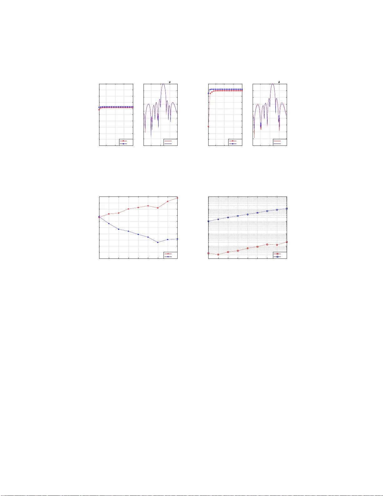
MIMO radar w a v eform design with practi cal constra in ts: A low-complexi t y approac h Chenglin Ren a, ∗ , F an liu a , Longfei Zhou b , Jianming Zhou a , W u Luo b , Shengzhi Y ang a a Scho o l of Information and Ele ctr onics, Beijing Institute o f T e chnolo gy, Beij ing 100081, China b State Key L ab or atory of A dvanc e d Optic al Communic ation Syst ems and Networks, Peking University, Beijing 100871, China Abstract In this letter, we consider the m ultiple-input mult iple-output (MIMO) radar wa veform design in the presence of signa l-dep endent clutters and additive white Gaussian noise. By imposing the constan t mo dulus constr a int (CMC) and wav e- form simila rity constraint (SC) , the signal-to- interference-plus-no ise (SINR) max- imization problem is non-conv ex and NP-ha rd in general, whic h ca n b e trans- formed into a seq ue nc e of conv ex quadr atically co nstrained quadra tic prog ram- ming (Q CQP) subpro blems. Aiming a t solving eac h subproblem efficien tly , we prop ose a lo w-complexity metho d termed Accelerated Gradient P ro jection (A GP). In cont rast to the conv entional IPM based metho d, our pro po sed a l- gorithm achiev es the same perfor mance in terms of the receive SINR and the bea mpattern, while notably reduces c omputational co mplexit y . Keywor ds: MIMO r adar, W a veform design, Constant mo dulus cons tr aint (CMC), Similar ity constra in t (SC), Signal-to-interference-plus-no ise (SINR), Quadratica lly constra ined quadra tic pr ogramming (QCQ P) 1. In tro duction MIMO radar has been intensively studied as a new paradigm of the radar system [1, 2, 3, 4]. By allowing individual wa veforms to b e transmitted at each antenna, MIMO ra dar is a ble to ex plo it extra deg r ees of freedo m in contrast to its phased-a rray counterpart, and therefore achieves a more fav orable per for- mance. In the existing literature [5 , 6, 7 , 8], radar wav efo r m optimization c an be classified into t wo catego ries: wav efor m design by only consider ing the radar transmitter [5, 6] and wa veform desig n by jointly co ns idering r adar transmitter and receive filter [7 , 8], where we fo cus on the seco nd categor y . ∗ Corresp onding author Email addr ess: rencl3@bit.edu. cn (Chenglin R en) Pr eprint submitte d to Signal Pr o c essing May 11, 2018 Pioneered b y the exploration of [9], the transmit wa veform is designed by maximizing the r e c eive SINR in the pr esence of the signal- dependent clutters and the Gaussia n no ise. In practice, for the use of non-linea r power amplifiers in the numerous ra dar systems, the CMC is typically involv ed, which is imp ortant to the SINR p er formance of the ra dar [9]. In a ddition, the SC enables a flexible tradeoff be tw een the output SINR and the desir ed auto co rrelation prop erties by co nt rolling the s imilarity b etw een the refer ence wa veform and its optimized counterpart. How ever, the wa vef orm design with b oth CMC and SC leads to the non-conv exity a nd the NP-hardness of the pro blem. T o overcome suc h a challenge, the previous w o rks [1 0, 11] either omit or rela x these constra ints in fav our of the existing solvers, which result in sub optimal s olutions and high computational co sts. Inspired by the r ecent resea rch [11], where the non-co nvex w av efo r m des ig n problem is r elaxed to a sequence of conv ex Q CQP subproblems, w e develop in this letter a different iterative r elaxing scheme to pr o duce the sequen tial QCQP subpro ble ms and a nov el AGP a lgorithm to solve ea ch s ubproblem. F ur- thermore, the pr o p o sed AGP in volv es tw o parts: the fast iterative shrink age- thresholding algo rithm (FIST A) pro cedure and the customized pro jection pro- cedure, where the former is based on the co n vex optimiza tion theory and the latter is hig hly dep endent o n the s pecific feasible r egion formulated by the CMC and SC. In contrast to the conven tional IP M that is employ ed in [11], o ur pro- po sed algorithm obtains a comparable per formance in terms of the receive SINR as well as the b eampattern. In addition, the AGP share s a m uch low er co mpu- tational complexity , and directly solves the complex conv ex QCQ P subproblems without co n verting them into the real repres e n tations [1 1]. 2. System Mo del W e consider a colo cated narrow ba nd MIMO radar s y stem with N T trans- mit a nt ennas and N R receive ant ennas. W e supp ose that t = [ t T 1 , ..., t T N ] T ∈ C N T N × 1 is the vectorized tra nsmit wa vform, where ( · ) T denotes the tr a nsp ose, N is the num b er of samples, and t n ∈ C N T × 1 , n = 1 , ..., N , stands for the n - th sample a cross the N T antennas. Then the receive wa veform r ∈ C N R N × 1 is given by [8] r = α 0 M ( φ 0 ) t + M X m =1 α m M ( φ m ) t + n (1) where n ∈ C N R N × 1 stands for the cir cular complex white Gaussian noise with zero mean and cov ariance matrix σ 2 n I , α 0 and α m represent the complex ampli- tudes of the targ et and the m -th interference so urce, φ 0 and φ m are the angle o f the target and the angle o f the m - th interference source, resp ectively , M ( φ ) de- notes the steer ing matrix of a Uniform Linear Array (ULA) with half-wav elength separatio n b etw een the antennas, which is given by M ( φ ) = I N ⊗ [ a r ( φ ) a t ( φ ) T ] (2) 2 where I N is the N × N iden tity ma trix, ⊗ deno tes the K roneck er pro duct, a t and a r are the trans mit and the receive steering vectors, r esp ectively . As men tioned above, aiming for maximizing the output SINR, w e propose to jointly optimize the tr a nsmit wa veform and the receive filter. Without loss of generality , we employ a linear Finite Impulse Respo nse (FIR) filter f ∈ C N R N × 1 to pro cess the received echo wa ve. This is given as r = f H r = α 0 f H M ( φ 0 ) t + M X m =1 α m f H M ( φ m ) t + f H n (3) where ( · ) H denotes the Her mitian transp ose. As a result, the output SINR can be expr essed as SINR = σ   f H M ( φ 0 ) t   2 f H ˜ S ( t ) f + f H f (4) where σ = E [ | α 0 | 2 ] /σ 2 n , with E [ · ] b eing the statistica l ex p ecta tion, and ˜ S ( t ) = M X m =1 I m M ( φ m ) tt H M H ( φ m ) (5) where I m = E [ | α m | 2 ] /σ 2 n . 3. Problem F orm ulation F ollowing the appro ach in [1 1], we incor po rate the CMC and SC in the max - imization of the output SINR , resulting in an o ptimiza tion pr o blem as follows max f , t σ   f H M ( φ 0 ) t   2 f H ˜ S ( t ) f + f H f s.t. | t ( k ) | = 1 / p N T N k t − t 0 k ∞ ≤ ε (6) where t ( k ) is the k -th e n try o f t , k = 1 , ..., N T N , k·k ∞ denotes the infinity norm, and t 0 represents the re ference wa veform. By taking int o account the CMC, the SC can b e r ewritten as arg t ( k ) ∈ [ ω k , ω k + δ ] (7) where ω k and δ are res pec tively given by ω k = a rg t 0 ( k ) − ar ccos (1 − ε 2 / 2) δ = 2 arcco s(1 − ε 2 / 2) (8) where t 0 ( k ) is the k -th ent ry of t 0 , and the prespecified parameter ε ( 0 ≤ ε ≤ 2) stands for the s imila rity b etw een t and t 0 . In a ddition, noting that f is 3 unconstrained [8], the optimization o f (6) is equiv alent to max t t H Ψ ( t ) t s.t. | t ( k ) | = 1 / p N T N arg t ( k ) ∈ [ ω k , ω k + δ ] (9) where Ψ ( t ) is a positive-semidefinite ma trix in terms of the output SINR and is given by Ψ ( t ) = M H ( φ 0 )[ ˜ S ( t ) + I ] − 1 M ( φ 0 ) . (10) According to the previous study [9], it is p o ssible to obtain a sub optimal SINR by assuming Ψ = Ψ ( t ) with a fixed t a nd optimizing t with the new Ψ iteratively . How ever, even for a fixed Ψ , the optimization o f t is still non-co nv ex and NP- hard due to the equality co nstraints inv o lved. In the next section, by referr ing to the metho d of Successive QCQP Refinement—Binary Sea rch (SQR-BS) [11], we introduce a low-complexity algo rithm to so lve (9). 4. Prop osed Al gorithm As analyz ed a b ove, we denote P = ( Ψ − λ I ), wher e I is a identit y matrix, λ ≥ λ max ( Ψ ) and λ max ( Ψ ) is the maximum eige nv alue of Ψ , which guara nt ees that P is negative-semidefinite. Hence, the o ptimization problem of (9) is equiv alent to the following non-conv ex pro blem max t t H Pt s.t. | t ( k ) | = 1 / p N T N arg t ( k ) ∈ [ ω k , ω k + δ ] . (11) It is easy to see that the feasible regio n for each entry of t can be viewed a s a circular arc from A to B as shown in Fig ure 1. F or notationa l co nvenience, we denote x k = Re( t ( k )), y k = Im ( t ( k )). The optimization problem o f (11) can b e relaxed as the fo llowing co n vex QCQP pr oblem max t t H Pt s.t. | t ( k ) | ≤ 1 / p N T N c x x k + c y y k ≥ c 2 x + c 2 y (12) where c x = cos( ω k ) + cos ( ω k + δ ) 2 c y = sin ( ω k ) + sin( ω k + δ ) 2 (13) represent the abscis sa and the ordinate of the p oint C, res pectively , as shown in Figur e 1 . The fea sible r egion of each t ( k ) is lab eled by zone I, which is the conv ex hull comp os ed by the circular arc a nd the line se g ment . 4 Figure 1: F easible r egion f or each di mension. Noting that the relaxatio n b ecomes clo ser to (11) a s the v alue o f δ b ecomes smaller, the author of [11] reduces δ by half and equally divides the feasible region into tw o parts. By itera tively selecting the part in which the optimized t lo cates and fixing P with a g iven t as analyzed in the last section, the se q uent ial conv ex QC Q P subproblems in the form of (12) are obta ined. The num b er o f times of dividing is given in adv a nce, and ea ch dividing is ca lled one refinement where the r esult is iteratively ca lculated via the conv ent ional IP M, which we refer r eaders to [1 1] for more details. F or clar it y , here we note the following tw o remar ks: (1) Rema rk 1 : Compare d with the SQR-BS algor ithm in [11], we do not fix the nu mber of the refinements which is equa l to itera tions, a nd reduce δ until it is sufficiently small. (2) Rema rk 2 : It is w orth highlighting that the feasible reg ion in (12) is conv e x , which enables a closed-for m pro jector to b e used in the gradient pro jection metho d. W e hereby pr op ose the AGP a pproach that inv o lves of tw o steps: the FIST A pro cedur e and the pro jection pro cedure. In the first step, we compute the gr a dient o f the ob jective function, and o btain the des cent di- rection b y the FIST A metho d. Then we pro ject the obtained p oint onto the feasible region by a sp ecifically ta ilo red orthog o nal pro jector. In what follows, we discuss the details of the AG P algor ithm. 4.1. FIST A Pr o c e dur e The FIST A pro cedur e acceler ates the iterative shr ink age-thresho lding algo- rithm (IST A) by introducing a smart in terp olation factor, which lea ds to a faster conv er gence rate c o mpared to that of the IST A metho d [12]. Both algor ithms are computationa l- efficient for unco nstrained co nv ex optimizatio n problems. Firstly , w e deno te y ( t ) = t H Pt , and then the g radient o f the ob jective function in (12) can b e caculated as g ( t ) = ∇ t y ( t ) = ( P + P H ) t = 2 Pt (14) 5 since P is a Hermitian matrix. Secondly , we der ive the Hessian ma trix as H = ∂ 2 y ( t ) ∂ t ∂ t H = P + P H = 2 P . (15) Thirdly , we s e t the stepsize τ = 1 /λ max ( H ), where λ max ( H ) is the maximum eigenv alue of H , na mely the Lipschitz consta n t o f the o b jective function. As a result, the iterative pro cedure ca n b e simply des c r ib ed as v ( n ) = t ( n ) + c k ( t ( n ) − t ( n − 1) ) t ( n +1) = v ( n ) − τ · 2 Pv ( n ) (16) where c k = ( k − 1 ) / ( k + 2 ) is the int erp olation factor, and v is the transitive vector. 4.2. Pr oje ction Pr o c e dur e As discussed ab ov e, we a ssume that the optimization is unconstr ained, i.e., the feasible r egion is the whole complex pla ne for each t(k). Inspired by [13], we design a pro jection pro cedure tha t pro jects each t ( k ) onto the zone I as shown in Figure 2. In what follows, we derive the pro jector under the tw o p oss ible cases, i.e., the angle δ corre s po nding to the zone I is less or gre a ter than π . (a) (b) Figure 2: Pro jection pro cedure for eac h dimension. (a) δ ≤ π ; (b) δ ≥ π . When δ ≤ π , as shown in Figure 2 (a), the r eal and the imaginar y axes are lab eled by x k and y k , resp ectively . The t wo extre me po in ts o f zone I are ma r ked with A ( a x , a y ) and B ( b x , b y ), re s pec tively , given by a x = cos( ω k ) , b y = s in( ω k ) b x = c o s( ω k + δ ) , a y = sin( ω k + δ ) (17) and C ( c x , c y ) denotes the midpo int o f line segment AB as defined in (1 3). Then we dr aw tw o radial lines l A and l B which are b oth vertical to AB and start at 6 A and B , r esp ectively , a nd furthermore, by adding the radia l lines O A and O B , the whole co mplex plane C is divided into 5 zo nes, i.e., I, I I, I I I( A ), I II( B ), IV. Given any Q ( x k , y k ) ∈ C , we can obtain the nearest p oint R ( x ∗ k , y ∗ k ) ∈ I via the pro jection pro cedure. If Q ∈ I, the pro jection is itself; if Q ∈ I I, R is the fo ot of the p erp endicular with AB thr o ugh Q ; if Q ∈ I I I( A ) or Q ∈ I I I( B ), the nea rest po int is A or B , resp ectively; if Q ∈ IV , R is the norma liz ation of Q . T o s um up, the pro jection can b e formulated as R =                      Q, c x x k + c y y k ≥ c 2 x + c 2 y , | OQ | ≤ 1 , F, c x x k + c y y k ≤ c 2 x + c 2 y , k l x k + d B ≤ y k ≤ k l x k + d A , A, a y x k − a x y k ≤ 0 , y k ≥ k l x k + d A , B , b y x k − b x y k ≥ 0 , y k ≤ k l x k + d B , Q/ | OQ | , othe rs (18) where k l = ( a y + b y ) / ( a x + b x ) repres e nts the slop e of l A and l B , d A = a y − a x k l and d B = b y − b x k l represent the in tercepts of l A and l B , r esp ectively , and F ( x f , y f ) is the fo ot of the p erp endicular o n AB , which ca n b e expressed as x f = c 2 x + c 2 y − c y ( y k − k l x k ) c x + k l c y y f = c 2 x + c 2 y − c x x f c y . (19) Particularly , if c x = 0 , F = ( x k , c y ); if c y = 0, F = ( c x , y k ). When δ ≥ π , as shown in Figure 2 (b), following the similar pro cedur e of (18), the pro jection can b e der ived as R =                      Q, c x x k + c y y k ≤ c 2 x + c 2 y , | OQ | ≤ 1 , F, c x x k + c y y k ≥ c 2 x + c 2 y , k l x k + d B ≤ y k ≤ k l x k + d A , A, a y x k − a x y k ≤ 0 , y k ≥ k l x k + d A , B , b y x k − b x y k ≥ 0 , y k ≤ k l x k + d B , Q/ | OQ | , othe rs. (20) where the only differences comparing with (18) ar e the signs of ine q ualities when Q ∈ I whe r e Q ∈ I I, and F ( x f , y f ) can b e also calculated by (19). F or clar ity , we summarize the prop o s ed a pproach for solv ing the QCQP subproblems in Algorithm 1. R emark 3 : The complex ity of the AGP mainly comes from the computation of the FIST A in (16) with 3 N 2 T N 2 + 3 N T N complex flops and the tailored pro- jection with 42 N T N complex flops, leading to a to tal co mputational c omplexity of O ( N 2 T N 2 ) for each iteration. F or conv erging to a sub optimal solution, the iteration num b er ne e de d for the pr op osed alg orithm is O (log (1 /ζ )) where ζ is 7 Algorithm 1 Accelera ted Gradient P ro jection (AGP) Require: P , t 0 , ζ (the desired thre s hold v alue), Num (the ma ximum num b er of iterations ), δ and ω k , k = 1 , ..., N T N . Compute g ( t ), t , Set n = 1, t (1) = t (0) = t 0 , Compute t (2) and it’s pro jection t (2) ∗ , Set n = n + 1 , while t ( n ) ∗ − t ( n − 1) ∗ > ζ and n < Num do Compute t ( n +1) by (1 6), for k = 1 , ..., N T N do Pro ject t ( n +1) ( k ) to t ( n +1) ∗ ( k ) with the given δ , ω k , k = 1 , ..., N T N to get the pro jection t ( n +1) ∗ end for Set n = n + 1. end whil e Ensure: t ∗ = 1 / √ N T N exp( j arg( t ( n ) ∗ )) for pro blem (11). the desired threshold v alue. O n the other ha nd, the computationa l co sts for the IPM is O ( N 3 . 5 T N 3 . 5 ) [14] and the num b er of iterations is O (log (1 /ζ )) as well [15]. 5. Numerical Re s ults In this s ection, we provide numerical r esults to ev aluate the p erfor mance in ter ms of the SINR and the b eampattern P ( φ ) b etw een the AGP and the IPM, and us e chirp wav efor m as our b enchmark. The referenc e wav efor m t 0 ∈ C N T N × 1 can be obtained by stacking the c olumns of T 0 , which is the orthog onal chirp wa veform matrix defined as T 0 ( k , n ) = exp[ j 2 π k ( n − 1) / N ] exp[ j π ( n − 1) 2 / N ] √ N T N (21) where k = 1 , ..., N T , n = 1 , ..., N . W e a ssume the num b er of samples N = 16, and the num b er of tra nsmit and the r e c eive antennas N T = 4, N R = 8 resp ec- tively . In addition, we co ns ider a scenario with three fix ed s ignal-dep endent clutters and additive white Ga ussian disturbance with v aria nce σ n = 0dB. The power of the tar get echo a nd the three interfering sources ar e | α 0 | 2 = 10 dB, | α 1 | 2 = | α 2 | 2 = | α 3 | 2 = 30 dB, r esp ectively , a nd the angle of the target and the three interferences are φ 0 = 15 ◦ , φ 1 = − 50 ◦ , φ 2 = − 10 ◦ , φ 3 = 4 0 ◦ , r esp ectively . W e first show the p erformance o btained by the tw o approa ches in Figur e 3 in terms of the SINR a nd the b eampa ttern. When ε = 0 . 4, Figure 3 (a) s hows very close SINR results of the b oth appro aches, while the b eampattern r esulting form the IP M ex hibits b etter suppression p erformance. As the similar it y lo os e , the b eampattern of the AGP outp erfor m the IPM when ε = 1 . 2 as shown in Figure 3 (b), a nd the difference o f the SINR is less than 0 .25dB. 8 5 10 15 20 Iteration index 10 11 12 13 14 15 16 17 18 19 20 SINR [dB] SINR per iteration AGP IPM -50 0 50 Angle [Degrees] -90 -80 -70 -60 -50 -40 -30 -20 -10 0 SINR [dB] Beampattern P( ) AGP IPM (a) 5 10 15 20 Iteration index 10 11 12 13 14 15 16 17 18 19 20 SINR [dB] SINR per iteration AGP IPM -50 0 50 Angle [Degrees] -90 -80 -70 -60 -50 -40 -30 -20 -10 0 SINR [dB] Beampattern P( ) AGP IPM (b) Figure 3: The SINR in eac h iteration and the beampattern P ( φ ) of the optimal wa ve form for the AGP and the IPM approac hes: (a) ε = 0 . 4; (b) ε = 1 . 2. 4 6 8 10 12 14 16 18 20 Number of transmit antennas 10 11 12 13 14 15 16 17 18 19 20 SINR [dB] AGP IPM (a) 4 6 8 10 12 14 16 18 20 Number of transmit antennas 10 -1 10 0 10 1 10 2 10 3 10 4 Time [sec] AGP IPM (b) Figure 4: (a) The SINR with increasing transmit an tennas. (b) The CPU time with increasing transmit antenn as. W e further co mpa re the SINR and the execution time of increasing transmit antennas for b oth approa ches in Figure 4, w he r e all the parameter s rema in the same with that of Figure 3 but ε = 0 . 5. Figur e 4 (a ) indicates the A GP obta in the notably sup erior p erformance than I P M a s N T increases. In addition, the simulation is p erfor med on a n Intel Cor e i5-620 0U CPU @ 2.3 GHz 12GB RAM computer. As shown in Figure 4 (b), the av er age CPU time of the AGP is remark a bly s horter than the IPM for so lving the optimization problem of (11). 6. Conclusion A low-complexity gr adient pro jection approa ch has b een prop osed for solving the MIMO radar wav efo r m design problem with CMC and SC co nstraints. By relaxing the fea sible reg ion, the key pro jection pro cedure is elab ora tely devised on the bas is of the FIST A metho d. Numerical results reveal that the pro po sed A GP algor ithm p ossesses a sup erior p erforma nce in terms o f the SINR a nd the 9 bea mpattern compar ed with the conv entional IPM, w ith a muc h low er complex- it y . Ac knowledgemen t Authors wish to thank the supp ort by the National Natural Science F oun- dation of China under Pr o ject No. 6 17710 47. References [1] E. Fishler, A. Haimovic h, R. S. Blum, L. J. Cimini, D . Chizhik, R. A. V a lenzuela, Spatial diversity in rada r s-mo dels and detection per formance, IEEE T rans. Signal Pro c ess. 54 (3) (2006) 823–838. doi:10 .1109 /TSP.200 5.862813 . [2] A. M. Ha imovich, R. S. Blum, L. J. Cimini, MIMO rada r with widely separated an tennas, IEEE Signal Pro c ess. Mag. 2 5 (1) (2008) 116– 129. doi:10 .1109 /MSP.200 8.4408448 . [3] K. W. F o rsythe, D. W. Bliss, G. S. F a wcett, Multiple-input m ultiple-output (MIMO) ra dar: p erfor ma nce issues , in: Pro c. 38th Asilomar Conf. Signals, Syst. Co mput., 2004, pp. 310–31 5 V o l.1. doi:10 .1109 /ACSSC.2 004.1399143 . [4] J. Li, P . Stoic a, MIMO radar with colo cated antennas, IEEE Sig nal Pr o cess. Mag. 24 (5) (2007 ) 1 0 6–11 4 . doi: 10.110 9/MSP. 2007.904812 . [5] D. R. F uhrmann, G. S. Antonio, T ransmit b e a mforming for MIMO ra dar systems using signal cr oss-cor relation, IEE E T rans. Aer o sp. Electro n. Syst. 44 (1) (200 8) 171–1 86. doi:1 0.1109 /TAES.2008.4516997 . [6] Y. C. W ang, X. W a ng, H. Liu, Z. Q . Luo, On the design of constant mo dulus probing sig nals for MIMO radar, IEEE T rans. Sig nal Pro c e ss. 60 (8) (2012 ) 4432– 4438. doi:1 0.1109 /TSP.2012.2197615 . [7] A. Aubry , M. L o ps, A. M. T ulino, L. V enturino, On MIMO detection under non-gauss ian target scatter ing, IE EE T rans. Inf. Theo ry 56 (11) (2010) 5822– 5838. doi:1 0.1109 /TIT.2010.2068930 . [8] G. Cui, H. Li, M. Rangaswamy , MIMO radar wav efor m desig n with con- stant mo dulus and similarity constr aints, IEE E T rans. Signal P ro cess. 62 (2) (201 4) 343–3 53. doi:1 0.1109 /TSP.2013.2288086 . [9] B. F riedlander, W av eform desig n for MIMO radar s, IEEE T r ans. Aerosp. Electro n. Syst. 43 (3) (2007) 1227– 1238. doi:10 .1109 /TAES.20 07.4383615 . 10 [10] H. Zang, H. Liu, S. Zhou, X. W ang, MIMO r adar wa veform design inv olving receiving be a mforming, in: Pro c. IEEE Int. Rada r Conf. (Radar ), 2014, pp. 1–4. doi:1 0.110 9/RADAR.2014.7060447 . [11] O . Alday el, V. Mong a, M. Rangaswamy , Succes sive QCQ P refinement fo r MIMO radar wa veform design under practical constra int s, IE E E T rans. Sig- nal P ro cess. 64 (1 4) (2 0 16) 376 0 –377 4 . do i:10. 1109/T SP.2016.2552501 . [12] A. Beck, M. T eb o ulle, A fast iterative s hrink age- thr esholding a lg orithm for linear inv ers e pro blems, SIAM Jour nal on Imaging Sciences 2 (1) (2009) 183–2 02. doi:1 0.1137 /080716542 . [13] F. Liu, L. Zhou, C. Mas ouros, A. Li, W. Luo , A. Petropulu, T o- wards dualfunctional rada r-communication systems: Optimal w av e - form desig n, submitted to IEEE T rans. Signal P ro cess. Av ailable: ht tps://ar xiv.org/ abs/17 11.05220. [14] A. Aubry , A. D. Maio, M. Piezzo , A. F arina, M. Wicks, Cognitive design o f the r eceive filter and transmitted phase code in rev erb er- ating en v ironment, IE T Radar, Sonar, Navig. 6 (9) (2012) 822–8 33. doi:10 .1049 /iet- rsn.2012.0029 . [15] Z. q. Luo, W. k. Ma , A. M. c. So, Y. Y e, S. Zhang, Semidefinite relaxatio n of quadratic optimizatio n problems, IEE E Signal Pr o cess. Mag. 27 (3) (2010 ) 20–34 . doi:1 0.1109 /MSP.2010.936019 . 11