Spatial Field Reconstruction and Sensor Selection in Heterogeneous Sensor Networks with Stochastic Energy Harvesting

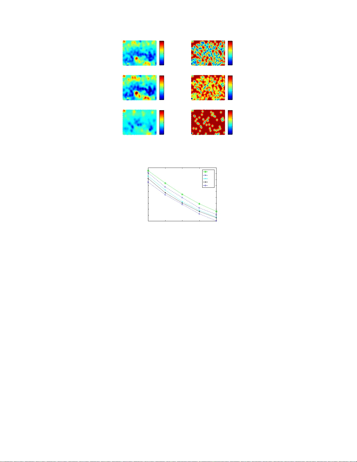
1 Spatial Field Reconstr uction and Sensor Selection in Heter ogeneous Sensor Networks with Stochastic Ener gy Harvesting Pengfei Zhang 1 , Ido Nevat 2 , Gar eth W . Peters 3 , Franc ¸ ois Septier 4 and Michael A. Osborne 1 1 Department of Engineering Science, University of Oxfor d, UK 2 TUM CREA TE, Sing apor e 3 Department of Actuarial Mathematics and Statistic s, Heriot-W att University , Edinburgh, UK 4 IMT Lille Douai, Univ . Lille, CNRS, UMR 9189 - CRIStAL, F-59000 Lille, France Abstract W e a d dress the two fundamental problems of spatial field reconstruction and sensor selection in het- erogeneous sensor networks. W e c onsider the ca se where two types of sensors are deployed: the first consists of expensive, h igh quality sensors; and the s econd, of cheap low quality sens ors, which are activated only if the intensity of the spatial field exc eeds a pre-defined activation threshold (eg. wind sensors). In addition, these sensors are powered by means of energy harvesting and their time varying energy status impacts on the a ccuracy of the measurement that may be obtained. W e account for this p henomenon by encoding the energy harvesting process into the second moment properties of the additive noise, resulting in a spatia l heteros cedastic process. W e then address the following two important p roblems: (i) how to efficiently pe r form sp a t ial field reconstruction based on measurements obtained simultaneously from both networks; a nd (ii) how to perform query based sensor set selection with predictive MSE performance guarantee . W e first show that the resultin g predictive posterior distribution, wh ich is key i n fusing such disparate observations, involves solving intractable integrals. T o overcome this problem, we solve the first problem by dev e loping a low complexity algorithm based on the spat ial best linear unbiased estimator (S-BL U E). Next, building on the S-BLUE, we address the second problem, and develop an efficient algorithm f or query base d sensor set selection with performance guarantee . Our algorithm is based on the Cross Entropy method which solves the combinatorial optimization p roblem in an efficient manner . W e present a comprehensive study of the performance gain that can be obtained by a ugmenting the high-quality sensors with low-quality sensors using both synthetic and real insurance storm surge database known as the Extreme W ind Storms Catalogue. DRAFT Keywords: Internet of Things, Sensor Networks, Gaussian Process, Energy harve sting, Cross Entropy method, Sensor selection I . I N T R O D U C T I O N W ireless Sensor Networks (WSN) have attracted considerable attention due to the large number of applica tions, such as environmental moni t oring [1], wea ther forecasts [2]–[4], s urv eillanc e [5], health care [6], structural sa fety and building monitoring [7] and home automati o n [4], [8]. W e consider a WSN whi c h consi sts of a set of spat ially dist ri buted sensors that may hav e limit ed r esources, suc h as energy and communi cation bandwidth. These se ns o rs monitor a spatial physical phenome non containing some des ired at tributes (e.g pressure, te mperature, conc entrations of subst ance, s ound intensity , radi ation levels , poll ution concentra tions, sei smic activ ity etc.) and r egularly com municate their ob servatio ns to a Fusion Centre (FC) [9]–[11]. The FC c o l lects these observat ions and fuses them in or der to reconstruct the spat ial field [8]. In many cas es these WSN use a sm all set of hi gh-quality a nd expensi ve sensors (such a s weat he r stations) [12]–[14 ]. While these sensors are capab l e of reliably me a suring the envi ronmental physical phenomenon, the lo w s patial deployment resolution pr ohib its their use in spatial fiel d r ec onstruction tasks. T o overcome this problem, sparse high-quality sensor deployme nt can be augmented by the use of complementa ry cheap low-quali ty sensors that can be d e ployed more densely due t o their low cos ts [2], [15]. This type of heterogeneo u s sensor networ ks approach has g a ined attenti on in the last few years due to the vi sion of the Internet of Things (IoT) where networks may share t he i r dat a over the internet [16], [17]. This coupli ng enab l es t he concept of Collaborative Wir eless Sens or Networ k (CWSN), in which networks wi th differ ent capabi l ities a re deployed in the same physi c al r egion and collab orate in order to optimize vari o us desi gn criteria and processes [18]. The incentive to develop such heterogeneous se ns o r ne t work and associated signal p rocessing was further strengthened when the US Environmental Pr otec tion Agency (EP A) publi shed its shift in the paradigm of data coll ection which promotes the notion of augme nt i ng sparse deploy m ents of hig h-quality sensors with dense deployment of low-quality and inaccura t e sensors [19]. T wo practic al scena ri os that are of importance are: 1) High-quality sensors may be deployed by government agencies (eg. weather stat i ons). These are sparsely deplo y ed due to thei r high costs, limit e d spa c e constraints, high power consumpti on etc. T o impr ove the c o verage of the WSN, low-quality cheap sensors can be deployed to augment the high-quality sensor network [15]. 2) High-quality se nsors c a nnot be easily deploye d in r emote locations, for example in oceans, lakes, mountains and volc anoes. In these cases, energy harves ting base d bat tery operated low-quality cheap sensors can be depl oyed [20]. In this paper we consider low-quality sens o rs which are capab le of measuri ng the i ntensity of the spatial random field, only if it e xc eeds a pre-defined threshold. For example, l ow cost wind se nsors are a b le t o mea s ur e the wind spee d only if it excee d s the ac tivati on threshold, se e for example [21], [22]. In ad dition, thes e se ns o rs are power ed by means o f ene rgy harvesting whic h impacts the i r reading accuracy . W e encode this aspect into the statisti cal properties of the addit ive noi se term, which r esults in a spatia lly correlated heteroscedastic process [23]. The FC then receives a vector of observati ons fr om both the high-quality a nd low-quality s e nsors. He nce, t he consequence is that the observati ons are heterogeneous and generally non-Gaussian distributed a s the activat ion threshold procedur e intr oduces a non-linear transformation of the observations, which make s the data fusion a more complex inference problem. The main goal of this pa per is to develop l ow com plexity algorithms to sol ve the problems of spatial field r econstruction and quer y base d sens o r set selection with per formance guaran te e of s p a tial random fiel ds in WSN under practic al scenarios of high and low qualit y sensors. Mor e specific ally , t he following two fundamental problems are the focus of this paper: 1) Spatial field reconst ruction : the task is to acc ura tely est i mate and predict the intensit y of a spatial random field, not only at the loca tions of the sensors, but at all lo cations [13], [24 ], [25], given heterogeneous o b servati o ns fr om both sensor networks. 2) Query based se n sor se t selection with performance guarante e : the task is to p e rform o n-li ne sensor set selec tion which meets the Q oS cri t erion impose d by the user , as wel l as mi ni mises the costs of acti vating the sensors of these networks [26]–[28]. A. Related work on spa tial field reconstruction in sen s or networ ks: It is com mon in the li terature to m odel the phys i cal phenomenon being monitored by the WSN according to a Gauss ian random field (GRF) with a spati al correlation st ructure [29 ]–[36]. More gen- erally , examples of G RFs include wireless c hannels [37], speech processing [38], na tural phenom ena (temperature, rai nfall i nt e nsity e tc.) [3], [39], and recently i n [24], [25]. The sim plest form of Gaussian process mod e l would typi cally assume t ha t the s patial field observed at t he FC is only corrupted b y additive Gaussian noise . For exampl e, i n [30] a linea r regr ession algorithm for GRF reconstruction i n mobile wireless sensor ne t works was presented, b ut relied o n the assumpti on of only Additive White Gaussian Noise (A WGN); in [40] an al gorithm was devel oped to learn the pa ra meters of non-stati o na ry spa t io-temporal GRFs agai n assum ing A WGN; and i n [41] an algorit hm for choosing sensor loca t ions in GRF a ssuming A WGN was devel oped. In practica l WSN d e ployments, two dev iations from these si m plified modell ing assump t ions arise and are important to consider: the use of heterogeneous sensor types i.e. sensors may have differ e nt degrees of ac curacy throughout t he field of spatia l monitoring [24], [25]; and secondl y quite often the sensors may b e power ed by means of ener gy harvesting which impacts thei r r eading accuracy and lifetime duration [35], [42]. In [26], the a ut hors deve loped an algori t hm for sensor sele c tion a nd power alloc ation in energy harvesting wireless s ensor networks. They extended the model proposed by Joshi and Boyd [27] and incorporated the energy harvesti ng pr ocess into t he problem form ul ation. Howeve r , they assumed that t he energy harves ting p rocess is fully observed , which is to o an opt i mistic as sumption in practice . In [28], [43], a s parsity-promoting penalty function to discourag e repeated sele ction of any sensor node was proposed. All of the s e works did not attempt to s o l ve t he senso r selecti on problem in heterogeneous sensor networks. Nor did the y as s ume that the energy harvesting process is not fully observ e d and impacts the reading acc ura cy of the sensors . Our pape r consi ders these i mportant as p e cts and provides both holistic and practica l solution for those problems. B. Contributions: 1) W e dev e lop a novel statis tical model to acc ount for high and low quality sensors (see A3-A4 in Section II-B). 2) W e model the prac tical s cenario of spatia lly correlated additi ve noise due to e nergy harve sting via a spati ally correlated heteroscedastic process (see A5-A6 in Sectio n II-B). 3) W e develop a point-wise estim ation algorithm for spati al field reconstruction which is ba sed on the Spatial Best Linear Unbia s ed Est imator (S-BLUE) (Corollary 1 in Sec tion II I-A). 4) W e develo p an ef ficient alg orithm to perform query base d s e nsor set selection with p erforman ce guaran te e which solves the com b inatorial optimizat ion problem using the Cross Entr opy method (Section IV). I I . S E N S O R N E T W O R K M O D E L A N D D E F I N I T I O N S W e begin b y pr esenting the statisti cal mod e l for the spati al phys ical phenom ena, foll owed by the system model. A. Spatial Gauss ian Ran dom Fie lds Background W e mod e l the physical phenome na (both monitored and energy harves ting phenomena) as spa tially dependent continuous processes wit h a spatia l correlation structure and are independent from each other . Such mo d els have r ece ntly b ecome pop ul ar due to their mathematical tracta b ility and a c curacy [33], [44], [45]. The deg r ee of the spatial correlation in t he process i ncreases with the decrease of the separation between two observ ing lo cations and can be acc urately mod elled as a Gaussian random field 1 [3], [24], [25 ], [29 ], [31 ], [37 ]. A Gaussian p rocess (GP) d efines a dist ribution over a s pace of functions and it is complet e ly sp ecified by the equivalent of suf ficient stati stics for s uc h a pr ocess, and is formally defined as follows. Definition 1 . (Gaus sian process [46], [47]): Let X ⊂ R d be some bounded do main of a d -di mensional r eal valued vector space. Denote b y f ( x ) : X 7→ R a stochastic pr oc e ss parametrized by x ∈ X . Then, the ra nd o m function f ( x ) is a Gaussian process if a ll its finite dime nsional distri butions are Gaussian, wher e for any m ∈ N , the random v ectors ( f ( x 1 ) , · · · , f ( x m )) are norm ally distribut e d. W e can therefor e interpr et a GP as formally defined by the followi ng class of ra ndom functions: F := { f ( · ) : X 7→ R s.t. f ( · ) ∼ G P ( µ ( · ; θ ) , C ( · , · ; Ψ )) , with µ ( x ; θ ) := E [ f ( x )] : X 7→ R , C ( x i , x j ; Ψ ) := E [( f ( x i ) − µ ( x i ; θ )) ( f ( x j ) − µ ( x j ; θ ))] , : X × X 7→ R + wher e at each poi nt the m e an of the function is µ ( · ; θ ) , para meterised by θ , and t he spat ial dependence between any two poi nt s is given by the cova riance function (Mercer ke rnel ) C ( · , · ; Ψ ) , parameteri sed by Ψ , see detaile d discuss ion in [46]. It will be useful t o make the following notati o na l definitions for the cross corr elation vec tor and auto-correlation ma t rix, respectivel y: k ( x ∗ , x 1:N ) := E [ f ( x ∗ ) f ( x 1:N )] ∈ R 1 ×N K ( x 1:N , x 1:N ) :=      C ( x 1 , x 1 ) · · · C ( x 1 , x N ) . . . . . . . . . C ( x N , x 1 ) · · · C ( x N , x N )      , with S + ( R n ) is the ma nifold of symm etric pos i tive definite matri ces. k ( x i , x j ) is the c o rr elation function and C ( x i , x j ) is the covaria nce functi on. W e define the Log Gaussia n Process (LGP) in the following definition: Definition 2. (Log Ga ussian process): A Log Gaus sian Process (LGP) d e fines a stochastic process wh ose logorithm follows Gauss ian Process. In mathematics, given a g ( x ) ∼ L G P ( µ g ( x ; θ g ) , C g ( x 1 , x 2 ; Ψ g )) . (1) where E [ g ( x )] = e µ g ( x ; θ g )+ C g ( x 1 , x 2 ; Ψ g ) 2 / 2 Having formally specified the semi-pa ra metric clas s of Gaussian process model s and Log Gauss ian process mod el, we pr oceed with presenting the sys tem m odel. 1 W e use Gaussian Process and Gaussian random field interch angeably . B. Heterogeneous Se nsor Network System Model W e now present the syst e m model for t he physical phenom e non obse rved by two types of networks and the energy ha rv esting model. A1 Consider a random spatial phenom enon (eg. wi nd) to be monitored defined over a 2 -dimensional space X ∈ R 2 . The mean r esponse of the physical process is a smooth c o nt i nuous spatia l functio n f ( · ) : X 7→ R , and is model led as a Gaus sian Pr ocess (GP) according to f ( x ) ∼ G P ( µ f ( x ; θ f ) , C f ( x 1 , x 2 ; Ψ f )) , (2) wher e the mea n and c o variance functi ons µ f ( x ; θ f ) , C f ( x 1 , x 2 ; Ψ f ) are as s umed to be known. A2 Let N be the total number of s ensors that ar e deploye d over a 2 -D region X ⊆ R 2 , with x n ∈ X , n = { 1 , · · · , N } b e ing the physical location of the n -th sensor , as s umed known by the FC. The number of sensors d eployed by Network 1 and Ne twork 2 a re N H and N L , r espective ly , so that N = N H + N L . A3 Sensor network 1 : High Quality Sens ors The sensors have a 0 -threshold activati o n and each of the s ensors collect s a noi sy observ ation of the spatia l phenome non f ( · ) . At the n -th sens or , locat ed at x n , the observati on is giv e n b y: Y H ( x n ) = f ( x n ) + W ( x n ) , n = { 1 , · · · , N H } (3) wher e W ( x n ) is i.i.d Gaussia n noise W ( x n ) ∼ N  0 , σ 2 W  . A4 Sensor network 2 : Low Qu a lity Sens ors The sensors hav e a T -thr eshold a ctivat ion and each of the sensors c ollects a noisy observati on of the spatial phe nom enon f ( · ) , only if the intensity of the field at that locati on exceed s the pre- defined t hreshold T , (eg. anem ometer sensors for wind monitoring [21], [22]). At the n -th sensor , located at x n , the obse rv ation is give n b y: Y L ( x n ) =    f ( x n ) + V ( x n ) , f ( x n ) ≥ T V ( x n ) , f ( x n ) < T (4) The statis t ical properties of the additiv e noise V ( x n ) are detailed i n A6. A5 Energy harves ting model: The energy harves ting p rocess (eg. solar irradianc e) is modelled as a spatial phenomenon defined over a 2 -dimens ional space X ∈ R 2 . The mean response of the physic al p rocess is a smo o th continuous spatia l function g ( · ) : X 7→ R , and in order to ens ure positivity it is m odelled as a log - Ga ussian Pr ocess (LGP), simi lar a s [32], [33], [35], [36], given by g ( x ) ∼ LG P ( µ g ( x ; θ g ) , C g ( x 1 , x 2 ; Ψ g )) . (5) W e ass um e that the e ne rgy harvesti ng process g ( x ) is independe nt of t he monitored physical phenomenon f ( x ) . 2 A6 Spatial noise process model: Since all sensors in Ne t work 2 use energy harvesting techniques fr om a spat i ally c orrelated energy fiel d g ( x ) , this will have a n impact on the performanc e of the ele ctronic circuits (eg. amplifiers, vol tage and frequency bias e s). These impact the therma l noise ( V ( x ) ) and its charac- teristic s, see [48]. As a r esult of the va riations and fluctuations of the energy field, the addi t ive thermal noi s e is now al s o spatially co rrelated across sensors e xpo sed to co m mon environmental energy harvesting conditions, such that E [ V ( x 1 ) V ( x 2 )] 6 = 0 . The spatial noise can be mode lled as a spatial stochastic volatility model in which the variance of the additive nois e is itself a random process which i s spat ially correlated. This means that if the energy harveste d by a particula r sensor is high, the noise varia nce should b e sm all and vice vers a . A common approach to modelli ng this impa ct i s via a link function as follows: σ 2 V ( x ) = ψ ( g ( x )) , (6) wher e ψ ( α ) : R + → R + is a deterministi c known m apping. The c hoice of ψ ( x ) c an b e fle xi ble in practice , but it nee d s to s atisfy the constrai nt s that the larger t he value o f x , t he smalle r ψ ( x ) is. Some choice of ψ ( x ) includes 1 /x, exp ( − x ) , 1 /x 2 and etc. In this paper , without loss of generality and for notational simpl icity , in the paper we assume that ψ ( α ) = 1 /α. In T able I we present t he notations which will be used throughout the pa per . T ABLE I: T a ble of Notations V ariable Meaning x 1:N physical locations in ter ms of [ x, y ] coordinates of th e N sensors deployed in the field. Y N = { Y 1 , . . . , Y N } ∈ R 1 × N collection of observations from all sensors (both Netw ork 1 and Network 2 ) at the fusio n center . Y H ∈ R 1 × N H ⊆ Y N collection of observations from all sensors in Network 1 at the fusion center . Y L ∈ R 1 × N L ⊆ Y N collection of observations from all sensors in Network 2 , at the fusion center . f N = { f 1 , . . . , f N } ∈ R N × 1 realisation of f at th e sensors located at x 1:N . f H ⊆ f N realisation of f at th e sensors of Network 1 , lo cated at x 1:N H ⊆ x 1:N . f L ⊆ f N realisation of f at th e sensors of Network 2 , lo cated at x 1:N L ⊆ x 1:N . g L = { g 1 , . . . , g N L } ∈ R N L × 1 realisation of the energy field G at the sensors of in Network 2 located at x 1:N L . 2 The e nergy harvesting and the physical phenomenon being measured would not be independent processes in some cases. In this paper however , we only consider t he case wh ere the energy harvesting model an d the physical phenomenon to be independent process, wh ich is of practica l importance in many cases. Some examples include energy ha rvesting via solar power and a phys ical p henomenon which is precipitation or pollution. I I I . F I E L D R E C O N S T R U C T I O N V I A S PA T I A L B E S T L I N E A R U N B I A S E D E S T I M ATO R ( S - B L U E ) T o perform i nfer ence i n our B a yesian framework, one would typica l ly be interested in computing the predictive posterior densit y at any l ocation in spac e, x ∗ ∈ X , denoted p ( f ∗ | Y N ) . Base d on this quantity various po int estim a tors, l ike the Mini m um Mean Squared Error (MMSE) and the Maximum A-Posteriori (MAP) estimat ors ca n be deriv ed: b f ∗ MMSE = ∞ Z −∞ p ( f ∗ | Y N , x 1:N , x ∗ ) f ∗ d f ∗ , b f ∗ MAP = arg max f ∗ p ( f ∗ | Y N , x 1:N , x ∗ ) . These estim ators provide a pointwi s e es t imator of the int e nsity of the spatial fiel d, b f ∗ at locat ion x ∗ . This enabl e s us to reconstruct the whole spatial field b y evaluat ing b f ∗ on a fine grid of points. The predictive posteri o r densi ty is given by: p ( f ∗ | Y N , x 1:N , x ∗ ) = Z R N p ( f ∗ | f N , x 1:N , x ∗ ) p ( f N | Y N , x 1:N , x ∗ ) d f N = Z R N p ( f ∗ | f N , x 1:N , x ∗ ) p ( f H , f L | Y H , Y L , x 1:N ) d f N = Z R N p ( f ∗ | f N , x 1:N , x ∗ ) Z R N L p ( f H | Y H , Y L , f L , x 1:N , g L ) × p ( f L | Y H , Y L , x 1:N , g L ) p ( g L | Y H , Y L , x 1:N , g L ) d g L d f N = Z R N p ( f ∗ | f N , x 1:N , x ∗ ) p ( f H | Y H , Y L , f L , x 1:N , g L ) × Z R N L p ( Y N | f L , x 1:N ) p  f L | x 1:N L  R R N L p ( Y N | f L , x 1:N , g L ) p  f L | x 1:N L  d f L p ( g L | Y H , Y L , x 1:N ) d g L d f N . (7) wher e R N L defines the domain for g L , which is t he N L dimensiona l LG P speci fied in A5 in Se ction II-B. Unfortunately , the predictive posterior de nsity cannot be calc ulated analyt ically in c losed form, prohibiting a direct calculation of any Ba yesian estim ator . One a pproach to approximating p ( f ∗ | Y N ) is t he Laplace a p p r oximation [49], which was used in our previous works [24], [25]. A dif fer ent approach is based on Markov Chain Monte C arlo (MCMC) methods which generates samples from the target distrib ut ion p ( f ∗ | Y N , x 1:N , x ∗ ) [23]. These methods are not suitable for our pr oblem as we requir e low c omplexity algorit hm which is suita b le for reconstructing t he whole s patial field a s well a s for select i ng the opt imal sub set of sensors i n real-time. In addi tion, expecta tion propagation and variationa l infer ence are unsuitable due to computational constraints. T o achieve these goals, we develop a low-comple xity linea r esti mator for f ∗ , presented next. A. Spatial Best Linear Unbiase d Es timator (S-BLUE) Field Reconstruction Algorithm W e develop the spatia l fiel d reconstruction via Best Linear Unbiased Estim ator (S-BLUE), which enjoys a low computational c o mplexity [50]. The S-BLUE do e s not require calc ul ating the predictiv e posterior dens i ty , but only the first two cross moments of the model. The S-BLUE is the optim al (in terms of mi ni mizing Mean Squared Error (MSE)) of all l inear estimat ors and is given by the solution to the following optimiz ation problem: b f ∗ := b a + b BY N = arg min a, B E h ( f ∗ − ( a + BY N )) 2 i , (8) wher e b a ∈ R and b B ∈ R 1 × N . The optimal linear esti mator that so lves (8) i s given by ˆ f ∗ = E f ∗ Y N [ f ∗ Y N ] E Y N [ Y N Y N ] − 1 ( Y N − E [ Y N ]) , (9) and the Mean Squared E rr or (MSE) is given by σ 2 ∗ = k ( x ∗ , x ∗ ) − E f ∗ Y N [ f ∗ Y N ] E Y N [ Y N Y N ] − 1 × E Y N f ∗ [ Y N f ∗ ] . (10) Remark 1. Non-zero mean random s patial pheno me non: in orde r to hand le the pra ctical case where µ f ( x ; θ f ) 6 = 0 , we first subtract this kno wn value from our observ ations Y H ( x n ) , and Y L ( x n ) . We then apply our algorithm, and finally shift back our results by µ f ( x ; θ f ) . T o ev aluate (9-10) we need to calculate the cross-correlation E f ∗ , Y N [ f ∗ Y N ] , auto-correlation E Y N  Y N Y T N  and E [ Y N ] . B. Cross-correlation between a test point and se nsors obse rvations E f ∗ , Y N [ f ∗ Y N ] T o ca lculate the cross-correlation vector , we decomp o se the obse rv ation vector into its high and low quality observat ions, give n b y: Y N = [ Y H , Y L ] , (11) and expr ess the cross-corr elation vector E f ∗ , Y N [ f ∗ Y N ] in (9-10) as: E f ∗ , Y N [ f ∗ Y N ] =  E f ∗ , Y H [ f ∗ , Y H ] | {z } q 1 , E f ∗ , Y L [ f ∗ , Y L ] | {z } q 2  (12) W e can now derive separatel y the cross-corr elation bet ween the t e st point x ∗ and a sensor observat i on fr om Network 1 and Network 2 . W e be g in with the d e rivation of the cross correlation be tween a test point f ∗ and the observat ions from sensors in Network 1 , Y H , presented in Lemma 1 followed by t he cross correlation between a test point f ∗ and observa tions fr om sensors in Ne twork 2 , Y L , presented in Lemm a 2. Lemma 1. (Calculating E f ∗ , Y H [ f ∗ Y H ] ): The cross co rrelation between a test p oint f ∗ and the k -th ( k = { 1 , . . . , N H } ) se nsor o bservation in Ne twork 1 is given by: [ q 1 ] k := E f ∗ ,Y H ( x k ) [ f ∗ Y H ( x k )] = k f ( x ∗ , x k ) . Proof. See Appendi x A Lemma 2. (Calculating E f ∗ , Y L [ f ∗ Y L ] ): The cr oss correlation between a test point f ∗ and the k -th ( k = { 1 , . . . , N L } ) se nsor obser vation in Network 2 is given by: [ q 2 ] k := E f ∗ ,Y L ( x k ) [ f ∗ Y L ( x k )] = C f ( x ∗ , x k ) × 1 − Φ T p C f ( x k , x k ) ! + T p C f ( x k , x k ) φ T p C f ( x k , x k ) !! . Proof. See Appendi x B Using Lemmas 1-2, the cross-correlation vect or q 1 , and q 2 in (12) is derived . C. Correlation of sensor s o bservations E Y N  Y N Y T N  W e now derive E Y N  Y N Y T N  , which is the correlation ma trix of all se nsors observa tions from both N e twork 1 and N e twork 2 . This i nvolves the c o rrelation within Network 1 and Network 2 and across the networks, giv en b y E Y N h Y N Y T N i = E Y H , Y L hh Y H Y T L i , [ Y H , Y L ] i =   E Y H  Y H Y T H  E Y H , Y L  Y H Y T L  E Y H , Y L  Y L Y T H  E Y L  Y L Y T L    :=    Q 1 Q 2 Q T 2 Q 4    . (13) Lemma 3. (Calculating E Y H  Y H Y T H  ): The cor relation between a se nsor obser vation in Networ k 1 , Y H ( x k ) ∈ Y H and a senso r observation in Network 1 , Y H ( x j ) ∈ Y H is given by [ Q 1 ] k ,j := E Y H ( x k ) ,Y H ( x j ) [ Y H ( x k ) Y H ( x j )] = k f ( x k , x j ) + 1 ( k = j ) σ 2 W . Proof. See Appendi x C Remark 2. Senso rs of h igh quality ha v e s patially uncorrelated thermal noise as no ene rgy harv e sting is requir ed, and the Dirac measure on the diagon a l wh en k = j . Lemma 4. (Calculating E Y H , Y L [ Y H , Y L ] ): The cor relation between a se nsor obser vation in Networ k 1 , Y H ( x k ) ∈ Y H and a senso r observation in Network 2 , denote d Y L ( x j ) ∈ Y L is given by [ Q 2 ] k,j := E Y H ( x k ) ,Y L ( x j ) [ Y H ( x k ) Y L ( x j )] = C f ( x k , x j ) 1 − Φ T p C f ( x j , x j ) ! + T p C f ( x j , x j ) ! φ T p C f ( x j , x j ) !! . Proof. See Appendi x D Next we de rive Q 4 , where we s e parate this calcul ation i nto two c ases: the d iagonal elem e nts of Q 4 are ca lculate d in Lemma 5, and the non-diagonal elements in Lemma 6. Lemma 5. (Calculating diago nal ele me nts of E Y L  Y L Y T L  ): The auto-correlation of se nsor o bservations in Network 2 , Y ( x k ) ∈ Y L is given by [ Q 4 ] k,k := E Y L ( x k ) [ Y L ( x k ) Y L ( x k )] = C f ( x k , x k ) 1 − Φ T p C f ( x k , x k ) ! + T p C f ( x k , x k ) ! × φ T p C f ( x k , x k ) !! + exp  µ g ( x k ) + C g ( x k , x k ) 2  . Proof. See Appendi x E . W e now co ns i der the calcul ation of the correlation between a single s e nsor observation in Network 2 , Y L ( x k ) ∈ Y L and a sensor observ ation in Network 2 , Y L ( x j ) ∈ Y L at differ e nt loc ations, (ie. non- diagonal elements x k 6 = x j ). This is given by [ Q 4 ] k ,j := E Y L ( x k ) ,Y L ( x j ) [ Y L ( x k ) Y L ( x j )] . T o ob tain this result, we first present the fol l owing Theorem whic h s tates useful results regarding the correlation of b i -variate truncated Norma l random variable s. Theorem 1 (Correlation of Biva riate T runcated Normal Random V ari ables [51 ]) . Given the standar dized bivariate Gaussian distribution Z = [ Z 1 , Z 2 ] , w h ere E [ Z 1 Z 2 ] = ρ , and observations available only inside the region [ a ≤ z 1 < ∞ , b ≤ z 2 < ∞ ] , the n the cross correlation E [ Z 1 Z 2 ] is given by: E [ Z 1 Z 2 ] = ∞ Z a ∞ Z b p ( z 1 , z 2 ) z 1 z 2 d z 1 d z 2 = ρ  aφ ( a ) (1 − Φ ( A )) + bφ ( b ) (1 − Φ ( B )) + Ω a,b  + (1 − ρ 2 ) f Z ([ a, b ]; ρ ) , where A = ( b − ρa ) √ 1 − ρ 2 , B = ( a − ρb ) √ 1 − ρ 2 , and Ω a,b := P ( Z 1 ≥ a ∩ Z 2 ≥ b ) is the joint co mplementary cumulative distribution function (CCDF), given by: Ω a,b := P ( Z 1 ≥ a ∩ Z 2 ≥ b ) = ∞ Z a ∞ Z b f Z ( z ; ρ ) d z 1 d z 2 = (1 − Φ ( a )) (1 − Φ ( b )) + φ ( a ) φ ( b ) ∞ X n =1 ρ n n ! H n − 1 ( a ) H n − 1 ( b ) , where Φ ( · ) the distribution function of a standard Ga ussian, a nd H n ( z ) are the Hermite-Chebysh ev polyno - mials orthogo nal to the stand ardized nor mal distribution such that ∞ Z −∞ He m ( z ) He n ( z ) e − z 2 2 d z = √ 2 π n ! δ nm , and He n ( z ) = ( − 1) n e z 2 2 d n dz n e − z 2 2 =  z − d dz  n · 1 , or explicitly as H e n ( z ) = n ! ⌊ n 2 ⌋ X m =0 ( − 1) m m !( n − 2 m )! z n − 2 m 2 m . Using Theorem 1 , we now derive the non-diagonal elements of Q 4 , pr esented in the follo wi ng Lemma: Lemma 6. (Calculating non -diagonal e lements of E Y L [ Y L , Y L ] ): The correlation be tween a single senso r obser vation in Ne twork 2 , Y L ( x k ) ∈ Y L and a sens or obse rvation in Network 2 , Y L ( x j ) ∈ Y L at different locations , (ie. x k 6 = x j ) is given by: [ Q 4 ] k,j = E Y L ( x k ) ,Y L ( x j ) [ Y L ( x k ) Y L ( x j )] = p C f ( x k , x k ) C f ( x j , x j ) C f ( x k , x j ) × ( T k φ ( T k ) (1 − Φ ( A )) + T j φ ( T j ) (1 − Φ ( B )) + Ω) + (1 − C 2 f ( x k , x j )) f Z ([ T k , T j ]; C 2 f ( x k , x j )) . where A = ( T j −C f ( x k , x j ) T k ) q 1 −C 2 f ( x k , x j ) , B = ( T k −C f ( x k , x j ) T j ) q 1 −C 2 f ( x k , x j ) . Proof. See Appendi x F D. Expected value of the obse rvations E Y N [ Y N ] Finally , we need to deriv e the expected va lue of the observa t ions for the high a nd l ow qualit y sensors. The expected value of the k -th ob servatio ns for a high quality sensor is given by: E [ Y ( x k )] = E [ Y ( x k ) + W x k ] = 0 . (14) Lemma 7. The expe cted va lue of the k -th obs ervations for a low quality sensor is presented in the following Lemma. E [ Y ( x k )] = E σ 2 V  E  Y ( x k ) | σ 2 V  = q C f ( x k , x k ) φ ( T k ) . Proof. See Appendi x G W e now use the results we deriv ed to express the S-BLUE for the spat ial field reconstruction in (9) and the associa t ed MSE in (10): Corollary 1. The S-BLUE spa tial field reconstruction at location x ∗ is given by: ˆ f ∗ =  q 1 q 2       Q 1 Q 2 Q T 2 Q 4      − 1      Y H Y L   −    E [ Y H ] E [ Y L ]       . The predictive va r iance is given by σ 2 ∗ = C ( x ∗ , x ∗ ) − [ q 1 q 2 ]   Q 1 Q 2 Q T 2 Q 4   − 1 [ q 1 q 2 ] T , (15) where q 1 , q 2 , Q 1 , Q 2 , Q 4 are given in Le mma 1, Lemma 2 , Lemma 3, Lemma 4, Lemma 5 a nd , Lemma 6, and E [ Y H ] and E [ Y L ] are give n in Eq. (14) and Lemma 7. There are sev eral quantities in this expression, q 1 , q 2 , Q 1 , Q 2 , Q 4 . Each of these quantity will pla y important r ole in determini ng the ˆ f ∗ . q 1 specifies the cross c orr elation between a test point f ∗ and the k -th ( k = { 1 , . . . , N H } ) sensor observa t ion in Network 1 , the higher this value , the l arger effect high qual ity s ensor ob servation have on ˆ f ∗ . Simila rly as q 2 , it specifies t he cross correlation betwee n a test poi nt and sensor observati on in Network 2 . Spec ifically , in summary , t he close t he tes t point to the s e nsor locati on in ei ther Network 1 or Network 2, the more effect will the sensor have on the estimat e d quantity at the test loca tion. I V . Q U E RY B A S E D S E N S O R S E T S E L E C T I O N W I T H P E R F O R M A N C E G U A R A N T E E In this Sec t ion we develop a n a lgorithm to perform o n-li ne sensor set selection i n o r der to meet the requir em e nts of a query made by users of the sy stem. In this scenario users can prompt t he s ystem and request the sy s tem t o provide an e stimated value of the spati a l rando m field a t a locat ion of interest x ∗ . The user al s o provides the requir ed al lowed error , quantified b y the Mean Squared Error (MSE) of the S-BLUE in Eq. (15). This means that the input to the syst e m is a pair of val ues indica ting the loc ation of interest, denoted b y x ∗ and the maxim al a llowed uncerta inty , denote d by σ 2 q . Our algorithm wi ll then choos e a subset of s ensors from b oth networks to acti vate in such a way t hat meets the QoS criterion (maxim al allowed unc e rtainty) a s well as minimises the costs of activ a ting the senso rs of these ne t works. It is i mportant to note that the MSE at any location can b e ev aluated without t a king a ny measurements, see (15 ). Thi s means tha t our algorithm for c hoo sing which sensors to activ ate does not requir e the se nsors to be acti vated b efor ehand. W e now formulat e the generic sensor se t sel ection problem where the se nsors from b o t h Network 1 and Network 2 are candi dates for activat ion. W e first define the user ’s query: Definition 3 . (User ’ s Query): A User ’ s Que ry consists of a 2-tuple Q := ( x ∗ , ε ) , wher e 1) x ∗ ∈ X ⊆ R 2 r epresents the locati on at which the user is interested in estimati ng the quantity of interest, denoted b f ( x ∗ ) . 2) ε ∈ R + r epresents the maxi m um stati stical error which the user is willing to a llow for the est i- mation of the quantity of interest a t x ∗ , quantified b y the MSE: E   b f ( x ∗ ) − f ( x ∗ )  2  , given in (15). Based on the query Q , the network out puts a report R :=  b f ( x ∗ ) , σ ∗  , with the c onstraint σ ∗ ≤ ε . If this condit ion cannot be m et, the network r eports a Null value and does not a ctivat e a ny se nsor configuration. W e defined the ac tivatio n sets of the sensors i n b oth networks by S 1 ∈ { 0 , 1 } | N H | , S 2 ∈ { 0 , 1 } | N L | . Then the sensor selec tion problem can be formulated as follows: S = arg min     S 1 ∈{ 0 , 1 } | N H | S 2 ∈{ 0 , 1 } | N L |     w h |S 1 | + w l |S 2 | , s.t. σ 2 ∗ < σ 2 q , (16) wher e σ 2 q is t he maxi mal allowed uncerta inty at the query lo c ation x ∗ , and w h and w l are the known costs of activati ng a sensor from Network 1 and Network 2 , respectiv ely . This optimi zation problem is not convex, due to the non-convex Boolean constra ints S 1 ∈ { 0 , 1 } | N H | , S 2 ∈ { 0 , 1 } | N L | . Solving this optimiza tion problem involv es e xhaustive eval ua tion of all possibl e co m binations of senso r selections which is im practica l for real-time applicati ons. Pr ev ious methods to solv e suc h o p timizat ion pr oblems in sensor sel ection inv olved a relaxation of the non-conve x c onstraint, s e e for exam p l e [26]–[28 ]. These approaches provide sub-optim al soluti ons and their t he oretical properties are not well understood. W e take a differ ent approach for sol ving the non-conv ex problem which does not inv olve relaxation, but instea d utilize a s tochastic optimiz ation tec hnique, known as the Cross Entropy Method (CEM). The CEM was first proposed by Rubinstein in 1999 [52] for rare event simula tion, b ut was adapted for solvi ng estima tion a nd optim ization problems see [52], [53]. W e now present a short overvie w of the CEM, for more deta i ls see [52], [53 ]. W e then develop the a lgorithm to s olve the opt imizati on problem in (16). A. Cross Entropy Method for Optimization problems Suppose we wish to maximiz e a function U ( x ) over some set X . L et us de note the maximum by γ ∗ ; thus, γ ∗ = max x ∈ X U ( x ) . (17) The CEM solves this optimiz ation problem by casting the original problem (17) into an estima tion problem of rar e-event pr obabil ities. By doing so, the CEM aims to locate an optima l paramet ric sam- pling dist ribution, that is, a probabil i ty d i stributi o n on X , rather than loca t ing the optimal sol ution directly . T o this end, we define a collect ion of indica tor functions { 1 { S ( x ) ≥ γ } } on X for various levels γ ∈ R . Next, l et { f ( · ; V ) , V ∈ V } be a fami ly of probability densitie s on X parametriz ed by a r eal- valued pa rameter vector v . For a fixed u ∈ V we ass ociate with (17) the p roblem of estim ating the rare-event probabilit y l ( γ ) = P u ( U ( x ) ≥ γ ) = E u  1 { U ( x ) ≥ γ }  , (18) wher e P u is the probability measure under which the random state x has a discrete pdf f ( · ; V ) and E u denotes the c orresponding expecta t ion operator . For a detaile d expositi o n of the CEM, see [52], [53]. The CE method involv e s the following itera tive pr ocedure shown in Al g orithm 1 : Algorithm 1 CE Met hod 1: Initi alizati on: Choos e an initial parameter vector V 2: while stoppi ng c riterion do 3: Generate K samples: Γ i , wher e Γ i ∼ f ( · ; V t ) ; 1 ≤ i ≤ K . 4: Evaluate U ( Γ i ) for all the K samples. 5: Calcula t e β t = (1 − ρ ) quantile of U 1 , . . . , U K 6: Solve the stoc ha stic program to update the parameter vect or V : V t = arg max V 1 K K X i =1 1 ( U ( Γ i ) ≥ β t ) ln ( f ( Γ i ; V t )) 7: end while The most chall e nging a spect in applying the CEM i s the se l ection of an appropriate cla ss of parametric sa mpling densiti es f ( · ; V ) , V ∈ V . There is not a unique parame tric family and the selecti on is guided by com p e ting objective s . The clas s f ( · ; V ) , V ∈ V has to be fl exible enough to include a r easonable parametri c a p pr oximatio n to the optimal importance sampling density . The density f ( · ; V ) , V ∈ V has t o be simple enough to allow fas t random vari able ge neration and closed-form solutions to the opti mizati o n problem. In addition, to be abl e to a nalytica lly solve the stochasti c program, then f ( · ; V ) should b e a mem ber of the Natural Exponenti al Famili es (NEF) of distri butions. Under NEF s, the optimiza tion problem can be sol ved a nalytica lly in closed form making the CE very easy to imple ment [53]. B. Cross Entropy Method for Sen s or Set Se lection T o apply the CEM to s olve our optimiza tion problem in (16), we need to choose a para metric distribut i on. Since the activati on of the sensors is a binary variable (eg. 0 → don’t ac tivate , 1 → activa te ), we choose a n i ndependent Bernoull i variab le as our parame t ric d istributi on, with a si ngl e parameter p (ie. V = p ). The Bernoulli distribution is a mem ber of the NEF o f distri b utions, hence, an analyti cal solution of the stoc hastic program is avai lable in cl osed form as foll ows: p t,j = K P i =1 1  Γ H i , j = 1  1 ( U ( k ) ≥ β t ) K P i =1 1 ( U ( k ) ≥ β t ) . Since the optimi zation problem in Eq. (16) is a constrai ned optimi zation problem, we introduce an Accept \ Reject step which rejects s a mples which do not meet the QoS criteri on σ 2 ∗ < σ 2 q , as follows U ( k ) =      −  w h   S H   + w l   S L    , σ 2 ∗ ( k ) < ǫ −∞ , Otherwise The resulting algori thm is pr esented in Algorithm 2. Our system mode l aims at ada p t ing the selection of the sensors according t o both the r equirements fr om the user (locati on of sensing and stati stical ac c uracy requir ed); as well as the bala nc e between activa ting high-quality and expensiv e senso rs (eg. wea ther stations) and low-quality cheap sensors. By “online” sens o r selection we mean that the system selects the “best” configuration of se ns o rs to activa te as a r esponse to a user ’s query which takes place in a r eal-time fashion. This dif fer entiates our problem fr om the so calle d “off-line” problem, where the sensors a re chosen once and do not change their operation in a responsive ma nner to user ’s querie s . V . S I M U L AT I O N S In this sec tion, we present extensive si m ulations to evalua t e the performance of the syste m. First, in Section V -A we p r esent the accura cy of the field reconstruction using our pr oposed S-BLUE al gorithm for synthetic dat a. Then in Section V -B we present results for the field reconstruction of r eal data set i n the form of wi nd storm. Final ly , in Se c tion V -C we present the effectiveness of using Cross Entropy base d al gorithm for s ensor selection and acti v ation. A. Field Recons truction of Syn the tic Data T o generate synthetic da t a, we used a Squa r ed E xponential kernel C f  x 1 , x 2 ; Ψ :=  σ 2 , l  = σ 2 exp  k x 1 − x 2 k 2 2 l  for both spatial random fields , f ( · ) and g ( · ) . The hyper-parameters for the random Algorithm 2 Sensor S e lection in Heterogeneous Sensor Networks via Cross Entropy met hod Require: User ’s query Q := ( x ∗ , ε ) , α , w h , w l and Ψ 0. Initiali z ation at ite ration t = 0 : s et p H 0 = { p H 0 , 1 , p H 0 , 2 , · · · , p H 0 ,N H } such that p H 0 ,j = 0 . 5 , and set p L 0 = { p L 0 , 1 , p L 0 , 2 , · · · , p L 0 ,N L } such that p L 0 ,j = 0 . 5 . while stopping criterio n do 1. Generate K independent samples of binary sets Γ H i = { γ H i, 1 , γ H i, 2 · · · , γ H i,N H } , where γ H i,j ∼ B er  p H t,j  ; 1 ≤ i ≤ K and Γ L i = { γ L i, 1 , γ L i, 2 · · · , γ L i,N L } , wher e γ L i,j ∼ B er  p L t,j  ; 1 ≤ i ≤ K . 2. Calculate the MSE v alues σ 2 ∗ ( k ) , k = { 1 , . . . , K } , which woul d be obtained by activ a ting t he corresponding s e nsors to each of the K sa mples, according to (15). 3. Evalua te for eac h of t he K samples the performance metric U ( k ) =      −  w h   S H   + w l   S L    , σ 2 ∗ ( k ) < ǫ ∞ , Otherwise wher e S H j =      1 , γ H j, 1 = 1 0 , Otherwise and S L j =      1 , γ L j, 1 = 1 0 , Otherwise 4. Calc ulate the β t = (1 − ρ ) quantile level of U 1: K . 5. Update p H as follows: p H t,j = α K P i =1 1  Γ H i , j = 1  Choose elite samples z }| { 1 ( U ( k ) ≥ β t ) K P i =1 1 ( U ( k ) ≥ β t ) + (1 − α ) p H t − 1 ,j , 6. Update p L as follows: p L t,j = α K P i =1 1  Γ L i , j = 1  Choose elite samples z }| { 1 ( U ( k ) ≥ β t ) K P i =1 1 ( U ( k ) ≥ β t ) + (1 − α ) p L t − 1 ,j , end while 7. For each element in p H and p L make the final binary acti vation dec ision as follows: S H j =      1 , p H t,j ≥ Ψ 0 , Otherwise and S L j =      1 , p L t,j ≥ Ψ 0 , Otherwise wher e Ψ is a pre-defined threshold. 8. Evaluate the objective functi on in (16) wit hout the se nsors which do not have e nough energy . If t he QoS c onstraint is met , then no further st eps a r e r equired; If the QoS constraint i s not met, solve the optimis ation problem again, excluding those sensors which were not a b le to transmit. spatial phenomenon f ( · ) are: Ψ f = { 10 , 1 } and for the e nergy harvesti ng field Ψ g = { 0 . 3 , 1 } . T he additiv e noise st andard deviati on is σ w = 1 , the mean is µ f = 8 . In Fig. 1, we present a single realisation of t he field intensity . In this example we deploye d 4 high quality a nd 64 l ow quali t y sensors uniformly in the rectangular r egion. In Fig. 2 we present the spati al fiel d r econstruction for various of activ ation speed s T = { 8 , 10 , 13 , 15 } . In Fig. 3 we present the point-wise Root Squar ed Error (RSE) for these T value s. Fi g . 3 illus trates that t he estimated wind field clo s ely mat c hes the true wind fiel d for small values of T and does not match the true wind field when T v a lues are high. W e al so obs erve that RSE decreases very fast with respect to increasing v alues of T . In a d dition, we observe that the RSE values are low in the region where many high a nd low quality sensors are distributed and high in the r egion where few high and low quality sensors are distributed. In Fig. 4 we present a quant i tative c omparison of RSE over 100 realizations from the spatial field with r espect of dif fer ent number of high qualit y and low quality sensors when T = 8 , as a function of t he number of l ow quali ty s e nsors. W e set the numbe r of high quali ty sensors to { 4 , 9 , 16 , 25 } and vary t he number o f lo w qual ity sensors from 4 t o 250 . The figur e s hows how a dding low qual i ty sensors aids in reducing the o v erall RSE. B. Field Recons truction of Stor m S u rge Data Set In order t o test our algorit hm on real data se t s, we us e a publicl y avail able i nsurance s torm s ur ge databas e known as the Extr eme W ind Storms C atalogue 3 . The data is a vailab le for r esearch as the XWS Data sets: (c) Copyright Met Office, Unive rsity of Readi ng and Universi ty of Exeter . Licensed under Creative Com m ons CC BY 4 . 0 Internationa l License . This data base is comprised of 23 sto rms which c a used high i ns ura nce losse s known as ‘insurance sto rm s’ and 27 storms which we re sel ected because they are the top ‘non-insurance’ storms as ra nked by the storm s everity index, see detai ls on the web site. The d a ta provided is co mprehensive a nd provides features such as the footprint o f the observatio ns on a locati o n grid with a rotated pole at longitude = 177 . 5 d e grees, latitude = 37 . 5 degrees. As dis cussed in the data descripti on provided with the dat a -set, this i s a standar d t echnique 3 http://www .met.reading.ac.uk/ extws/datab ase/dataDesc Wind field 0 2 4 6 8 x 0 1 2 3 4 5 6 7 8 9 y 0 2 4 6 8 10 12 14 16 Fig. 1: W ind field intensity T=8 0 2 4 6 8 x 0 2 4 6 8 y 0 5 10 15 T=10 0 2 4 6 8 x 0 2 4 6 8 y 0 5 10 15 T=13 0 2 4 6 8 x 0 2 4 6 8 y 0 5 10 15 T=15 0 2 4 6 8 x 0 2 4 6 8 y 0 5 10 15 Fig. 2: S-BLUE wind field reconstruction of Corollary 1 for differ ent acti vation speed thresholds T = { 0 , 2 , 5 , 7 } RSE T=8 0 2 4 6 8 x 0 2 4 6 8 y 1 1.5 2 2.5 3 RSE T=10 0 2 4 6 8 x 0 2 4 6 8 y 1 1.5 2 2.5 3 RSE T=13 0 2 4 6 8 x 0 2 4 6 8 y 1 1.5 2 2.5 3 RSE T=15 0 2 4 6 8 x 0 2 4 6 8 y 1 1.5 2 2.5 3 Fig. 3: Root Mean Squared Err or (RMSE) estim a tion of the wind fiel d intensity used to ensur e that the s pacing in k m be tween grid poi nts remains relatively consiste nt. The footprints are on a regular gri d in the r otated coordinate system, with horizontal grid spac ing 0 . 22 degrees. The dat a for eac h of the st o rm s provides a l ist of grid number and ma ximum 3 -second gust spe ed in meters pe r second. The true locatio ns (longi t ude and latitude) of the grid points are given in grid locatio ns file. W e selected o ne storm to a na lyse, known as D agmar which took pla ce o n 26/12/20 1 1 and affected Finland and Norway . T o calib rate t he model we first fit the hyperparamete rs of the model via Maxi mum Likel ihood Estimati on (MLE) pr ocedure. W e used a 2 -D radial basis function, of the following form C ( x i , x j ; Ψ ) := σ 2 x exp  − | x i − x j | l x  exp  − | y i − y j | l y  , thus decompo s ing the kernel into o rt hogonal coordinates which we found provided a much m ore accurate fit. The reason for this is it a llows for i nhomogeneity through differ enc e s in spatial depen- dence in vertical and horizont a l dir ections, which is highly likel y to occ ur in the types of wind spee d 5 50 100 150 200 250 Number of low quality sensors 1.5 2 2.5 3 RSE Number of high quality sensors =4 Number of high quality sensors =9 Number of high quality sensors =16 Number of high quality sensors=25 Fig. 4: RSE as a function differ ent configurations of number of high and low quality sensors High quality Low quality 0 5 10 15 20 25 30 35 40 Fig. 5: L e ft panel: map of region of interest wit h sensors loca tions. Right panel : Dagmar surge storm intensity map data studied. The MLE of the length a nd scale param eters obtained are g iven b y σ 2 x = 0 . 1 , l x = 0 . 5 and σ 2 y = 10 , l y = 0 . 1 . D e tails on how to estimate t he GP hyperpa rameters can be found in [Chapt e r 5] [46]. In our model , histori cal data is used in order to estimate the hyperparameters of the m odel at the current t ime. Then, using these parameters we perform all the inferential tasks. The left panel of Fi g . 5 shows the region of interest on the map. Both high and low qualit y sensors are s e lected ra ndo mly within the region. In this experiment we uniformly deployed 50 high quali t y and 250 low quality s ensors. The right panel of Fi g. 5 shows the Dagmar storm wind speed intensity . The left c olumn of Fi g . 6 presents t he esti mated wind speed inte nsity with va ry i ng ac tivatio n speed thresholds T and the right c olumn presents the spati a l RSE values. The figur e shows that the true wind intensity field can be recovered for low act ivation speed, but a s the threshold increases, the performance dete ri orates. The RSE is lower a t the p o i nts where sensors are de p loyed, and grows with the i ncrease of activa tion speed threshold. The st a ndard deviatio n is v e ry low i n t he middle region, clo se to a value of 2 and a b i t high in the boundary r egion where fewer sensors are de ployed. Finally , in Fig. 7 we present a quantitati ve comparison of the RMSE for v arious values of high and low qual i ty se nsors. The result shows a c lear trend of RMSE with the increasing of high and low quality sensors. C. Senso r Se le ction In this sec tion we illust rate how our sensor sel ection a l gorithm performs . For compariso n, we use a optimal sel ection me t hod which onl y sel ects the s e nsor set col lections that minim ize the U Estimated field, T=0 0 10 20 30 40 Estimated field, T=15 0 10 20 30 40 Estimated field, T=35 0 10 20 30 40 RMSE T=0 0 2 4 6 RMSE T=15 0 2 4 6 RMSE T=35 0 2 4 6 Fig. 6: T rue storm field and esti mated sto rm field with v arious activ a tion speed. 50 100 150 200 250 N l 4 4.2 4.4 4.6 4.8 5 5.2 5.4 5.6 5.8 RMSE N h =10 N h =20 N h =30 N h =40 N h =50 Fig. 7: RMSE with effect o f diff erent numb e r o f hi g h and low quality sensors. values a nd ensures that the Q oS cri terion is being met. The si mulation parame ters we have are: { N h = 5 , N l = 10 , T = 8 , w h = 150 , w l = 30 , σ w = 1 , σ g = 0 . 3 , k f ( x ∗ , x ∗ ) = 10 , x ∗ = 3 . 5 , y ∗ = 3 . 1 , ǫ = { 5 . 4 , 5 . 6 , 5 . 8 , 6 , 6 . 2 }} . W e fix the N h = 5 , N l = 10 . The compa rison is shown i n Fig. 8. W e chang e the ǫ withi n { 5 . 4 , 5 . 6 , 5 . 8 , 6 , 6 . 2 } . W e also increase the number of iterations in CE method fr om 1 to 10 . It shows CE method converges quickly to the optimal selecti on alg o rithm wit hin 10 iteratio ns for all the ǫ values . T o compare our method with convex optimiza tion approach, we foll owed a similar line of thought which was pr esented in [41]. W e com pared the performance of our CEM algorithm with the r elaxation- based optimiza t ion al gorithm. The result shows that for dif fer ent QoS, ǫ , our C EM has a s ignificant lower cost compared t o the c onvex optimiza tion scenari o , as shown in the figur e 9. V I . C O N C L U S I O N S W e addressed the problem of spatial field reconstruction and se nsor sel e ction in heterogeneous sensor networks, contai ning two t ypes of sensors: expensi ve, high quality sensors; and cheap, low quality sens o rs which a re activ a ted only if t he inte nsity of the spat ial field exceeds a pre-defined activa tion threshold. In add i tion, these sensors are powered by means of e ner gy harv esting which impacts their acc uracy . W e t hen addressed the problems of performing spatial field reconstruction a nd 1 2 3 4 5 6 7 8 9 10 Number of Iterations 0 100 200 300 400 500 600 U CE = 5.4 Opt = 5.4 CE = 5.6 Opt = 5.6 CE = 5.8 Opt = 5.8 CE = 6 Opt = 6 CE = 6.2 Opt = 6.2 Fig. 8: C o mparison of U va lues b etween optimal scheme a nd CE m ethod with ef fect of num b er of iterations . 1 2 3 4 5 6 7 8 9 10 Number of Iterations 100 200 300 400 500 600 700 800 U CE = 5.03 Convex = 5.03 CE = 5.04 Convex = 5.04 CE = 5.05 Convex = 5.05 Fig. 9: Compari son of objectiv e function va l ues b etween Convex o p t imizati on scheme and CE method. query based senso r set s e lection with performa nce guarantee . W e solved the first problem by developi ng a low complexity algorithm ba s ed on the spatial best linear unbias e d es timator (S-BLUE). Next, buil ding on the S-BLUE, developed an efficient algori thm for query bas ed sensor set se lection with perfor mance guaran te e , based on the Cross Entropy method which solve s the combinat o rial optimizati on pr ob lem in an ef ficient m anner . W e presented a comprehensive s tudy of the performance gain that can b e obtained by a ug menting the high-quality s ensors with low-quali t y sens o rs using both sy nthetic and real insurance sto rm sur ge datab a se known as the Extreme W ind Storms Catalog ue . A P P E N D I X A P R O O F O F L E M M A 1 Using the the l a w of t otal expectati on, the properties of the GP and the fact that f ( x k ) a nd W k are inde pendent, we obtain tha t: E f ∗ ,Y H ( x k ) [ f ∗ Y H ( x k )] = E f ∗ ,Y H ( x k ) [ f ∗ ( f ( x k ) + W ( x k ))] = E f ∗ ,f ( x k ) [ f ∗ f ( x k )] + ✭ ✭ ✭ ✭ ✭ ✭ ✭ ✭ ✭ ✭ E f ∗ ,f ( x k ) [ f ∗ W ( x k )] = k f ( x ∗ , x k ) . (19) A P P E N D I X B P R O O F O F L E M M A 2 E f ∗ ,Y L ( x k ) [ f ∗ Y L ( x k )] = E f ( x k ) ,σ 2 V ( x k )  E f ∗ ,Y ( x k )  f ∗ Y ( x k ) | f ( x k ) , σ 2 V ( x k )  = C f ( x ∗ , x k ) C f ( x k , x k ) E f ( x k ) ,σ 2 V ( x k )  f 2 ( x k ) 1 ( f ( x k ) > T )  = C f ( x ∗ , x k ) C f ( x k , x k ) ∞ Z 0 ∞ Z T f 2 ( x k ) N ( f ( x k ) ; 0 , C f ( x k , x k )) d f ( x k ) p ( σ 2 V ( x k )) d σ 2 V ( x k ) W e can derive E f ∗ ,Y L ( x k ) [ f ∗ Y L ( x k )] = C f ( x ∗ , x k ) C f ( x k , x k ) 1 p C f ( x k , x k )  p C f ( x k , x k )  3 × Φ f ( x k ) p C f ( x k , x k ) ! − f ( x k ) p C f ( x k , x k ) φ f ( x k ) p C f ( x k , x k ) !!    f ( x k )= ∞ f ( x k )= T = C f ( x ∗ , x k ) 1 − Φ T p C f ( x k , x k ) ! + T p C f ( x k , x k ) φ T p C f ( x k , x k ) !! . A P P E N D I X C P R O O F O F L E M M A 3 E Y H ( x k ) ,Y H ( x j ) [ Y H ( x k ) Y H ( x j )] = E f ( x k ) ,f ( x j ) ,W ( x k ) ,W ( x j ) [( f ( x k ) + W ( x k )) ( f ( x j ) + W ( x j ))] = E f ( x k ) ,f ( x j ) [ f ( x k ) f ( x j )] + E W ( x k ) ,W ( x j ) [ W ( x k ) W ( x j )] = k f ( x k , x j ) + 1 ( k = j ) σ 2 W . A P P E N D I X D P R O O F O F L E M M A 4 E Y H ( x k ) ,Y L ( x j ) [ Y H ( x k ) Y L ( x j )] = E f ( x j ) ,σ 2 V ( x j ) h E Y H ( x k ) ,Y L ( x j )  Y H ( x k ) Y L ( x j ) | f ( x j ) , σ 2 V ( x j )  i = E f ( x j ) ,σ 2 V ( x j ) h E f ( x k ) ,W ( x k ) ,V ( x j ) "  ( f ( x k ) + W ( x k )) ( f ( x j ) + V ( x j )) | f ( x j ) , σ 2 V ( x j )  # i = E f ( x j ) ,σ 2 V ( x j ) " C f ( x k , x j ) C f ( x j , x j ) f ( x j ) 2 1 ( f ( x j ) > T ) # Now we can follow the deriva tion i n Appendix B , and we can get E Y H ( x k ) ,Y L ( x j ) [ Y H ( x k ) Y L ( x j )] = C f ( x k , x j ) 1 − Φ T p C f ( x j , x j ) ! + T p C f ( x j , x j ) ! φ T p C f ( x j , x j ) !! . A P P E N D I X E P R O O F O F L E M M A 5 E Y L ( x k ) [ Y L ( x k ) Y L ( x k )] = E Y L ( x k ) ,V ( x k )  ( f ( x k ) + V ( x k )) 2 1 ( f ( x k ) > T )  = E f ( x k )  E V ( x k )  ( f ( x k ) + V ( x k )) 2 | f ( x k )  1 ( f ( x k ) > T )  = E f ( x k ) " E V ( x k ) h  f ( x k ) 2 + 2 f ( x k ) V ( x k ) + V ( x k ) 2 | f ( x k )  × 1 ( f ( x k ) > T ) i # = E f ( x k )  f ( x k ) 2 1 ( f ( x k ) > T )  + E V ( x k )  V ( x k ) 2  = C f ( x k , x k ) 1 − Φ T p C f ( x k , x k ) ! + T p C f ( x k , x k ) ! φ T p C f ( x k , x k ) !! + exp  µ g ( x k ) + C g ( x k , x k ) 2  . A P P E N D I X F P R O O F O F L E M M A 6 [ Q 4 ] k,j := E Y L ( x k ) ,Y L ( x j ) [ Y L ( x k ) Y L ( x j )] = E f ( x k ) ,f ( x j ) ,σ 2 V ( x k ) ,σ 2 V ( x j ) h ( f ( x k ) + V ( x k )) ( f ( x j ) + V ( x j )) × 1 ( f ( x k ) > T , f ( x j ) > T ) | σ 2 V ( x k ) , σ 2 V ( x j ) i (20) Note i n the above equatio ns, all the c ross moments te rm s relating to the product of V ( x k ) V ( x j ) , f ( x k ) V ( x j ) and f ( x j ) V ( x j ) will become zero since there is independe nce betwee n these terms. So the equation r educes to: [ Q 4 ] k,j = ∞ Z T ∞ Z T p ( f ( x k ) , f ( x j )) f ( x k ) f ( x j ) d f ( x k ) d f ( x j ) = E f ( x k ) ,f ( x j ) h f ( x k ) f ( x j ) 1 ( f ( x k ) > T , f ( x j ) > T ) i = E f s ( x k ) √ C f ( x k , x k ) ,f s ( x j ) q C f ( x j , x j ) h  f s ( x k ) p C f ( x k , x k )   f s ( x j ) p C f ( x j , x j )  × 1 ( f s ( x k ) > T k , f s ( x j ) > T j ) i = p C f ( x k , x k ) C f ( x j , x j ) ∞ Z T k ∞ Z T j p ( f s ( x k ) , f s ( x j )) f s ( x k ) f s ( x j ) d f s ( x k ) d f s ( x j ) = p C f ( x k , x k ) C f ( x j , x j ) E f s ( x k ) ,f s ( x j ) h f s ( x k ) f s ( x j ) i . (21) Finally , util ising Theorem 1 we obtain the result. A P P E N D I X G P R O O F O F L E M M A 7 E [ Y ( x k )] = E σ 2 V  E  Y ( x k ) | σ 2 V  = E σ 2 V  E  ( f ( x k ) + V ( x k )) 1 ( f ( x k ) ≥ T ) | σ 2 V + V ( x k ) 1 ( f ( x k ) < T ) | σ 2 V  = E σ 2 V [ E [ f ( x k ) 1 ( f ( x k ) ≥ T )]] = E σ 2 V  Z f ( x k ) p ( f ( x k )) 1 ( f ( x k ) ≥ T ) d f ( x k )  = E σ 2 V " 1 p C f ( x k , x k ) Z + ∞ T f ( x k ) φ f ( x k ) p C f ( x k , x k ) ! d f ( x k ) # = − p C f ( x k , x k ) φ f ( x k ) p C f ( x k , x k ) !!   ∞ T = p C f ( x k , x k ) φ ( T k ) . A C K N O W L E D G M E N T This work was suppor ted by the Korea Institute of Energy T echnology Evaluation and Planning (KETEP) and the Ministry of T rade, Industry & Energy (MOTIE) of the Republic of Korea (No. 201 4851001 1150). R E F E R E N C E S [1] J. K. Hart and K. Mar tinez, “Environmental Sensor Network s: A revolution in the earth system science?” Earth-Science Reviews , vol. 78 , no. 3, pp. 177 –191, 2006. [2] S. Rajasegarar , T . C. Havens, S. Karunasekera, C. Le ckie, J. C. Bezdek, M. Jamriska, A. Gunatilaka, A. Skvortsov , and M. Palaniswami, “High-Resolution Monitoring of Atmospher i c Pollutants Using a System of Low-Cos t Sensors,” IEEE T ransactions on Geoscience and Remote Sensing , vol. 52, pp. 382 3–3832, 2014. [3] C. Fo nseca and H. Ferreir a, “Stability and contagion measures for spatial extreme value analyses,” arXiv preprint arXiv:1206.122 8 , 2012. [4] J. P . French and S. R. Sain, “Spatio-T emporal Exceedance Locations an d Confidence Regions,” An nals of Applied S tatistics. Prepr ess , 20 13. [5] K. Soh raby , D. Minoli, and T . Z nati, Wir eless sensor networks: technology , pr otocols, and ap plications . John W iley & Sons, 2007. [6] K. Lorincz, D. J. Malan, T . R. F . Ful f o rd-Jones, A. Nawoj, A. Clavel, V . Shnayder , G. M ainland, M. W elsh, and S. M oulton, “Sensor networks for emergency response: challenges and opportunities,” IE EE Pervasive Computing , vol. 3, no. 4, pp. 16–23, 2004. [7] K. Chintalapudi, T . F u, J. Paek, N. Kothari, S. Rangwala, J. Caffrey , R. Govindan, E. Johnson, and S. M asri, “Monitoring civil structures with a wireless s ensor network,” Internet Computin g, IEEE , vol . 10, no. 2, pp. 26–34, 2006. [8] I. F . Aky ildiz, W . Su, Y . San karasubramaniam, and E. Cayirci, “W ireless sensor networks : a survey,” Computer Networks , vol. 38, no. 4, pp. 393–422, 2002. [9] F . Fazel, M. Fazel, and M. Stojanovic, “Random access sensor networks: Fiel d recon struction from incomplete d ata,” in IEEE Information Theory and Applications Workshop (IT A) , 2012, pp. 30 0–305. [10] J. Matamoros, F . Fabbri, C. Ant ´ on-Haro, and D. Dardari, “On the e stimation of randomly sampled 2d s patial field s under bandwidth constraint s,” IEEE T ransactions on Wir eless Commun ications, , vol. 10, no. 12, pp. 4184–4 192, 2011. [11] M. C. V uran, O. B. Akan , an d I. F . Akyildiz, “Spatio-temporal correlation: theory and applications for wireless sensor networks,” Computer Networks Journ al, Elsevier , vol. 45 , pp. 245–2 59, 2004. [12] “Environment Protection Authority V ictor i a Sensor Locations,” 2012. [ Online]. A vailable: http://www .epa.vic.gov .au/air/airmap [13] G. W . Peters, I. Nevat, and T . Matsui, “How to Utilize Sensor Network Data to Ef ficiently Perform Mo del Calibration and Spatial Field Re construction,” in Modern M ethodology and Applications in Spatial-T emporal Modeling . Springer , 2015, pp. 25–62. [14] G. Peters, I. Nevat, S. Lin, and T . Matsui, “Model ling threshold exceedence levels for sp atial stochastic processes observed by sensor networks,” in 2014 IE E E Nin th I n ternational Conference on Intel ligent S ensors, Sen sor Networks and Information Proc essing (ISSNIP) . IEEE, 2014, pp. 1– 7. [15] S. Raja segarar , P . Zhang, Y . Zhou, S. Karunasekera, C. Leckie, and M. Pa laniswami, “ High resolution spatio-temporal monitoring of air pollutants using wireless sensor networks , ” in 201 4 IEEE Ninth I n ternational Conference on Intelligent Sensors, Sensor Networks and In formation Pro cessing (ISSNIP) . IEEE, 201 4, pp. 1–6. [16] J. Gubbi, R. Buyya, S. Marusic, and M. Palaniswami, “Internet of Things (IoT): A vision, architectural elements, and future di rections,” Future Generation Computer Systems , vol. 29, no. 7 , pp. 1645– 1660, 2013. [17] O. V ermesan, P . F riess, P . Guil l emin, S. Gusmeroli, H. Sundmaeker , A. Bassi, I. S. Jubert, M. Mazura, M. Harr ison, M. E isenhauer , and Others, “Internet of things strategic research roadmap,” O. V ermesan, P . F riess, P . Guillemin , S. Gusmeroli, H. Su ndmaeker , A. Bassi, et al., Internet of Things: G l obal T echnological and Societal T rends , vol. 1, pp. 9–52, 2011. [18] C. Perera, A. Zaslavsky , C. H. Liu, M. Compton, P . Christen, and D. Georgakopoulos, “Sensor search techn iques for sensing as a s ervice arch itecture for the internet of things,” IEEE Sensors Journal , vol . 14, no. 2, pp. 406 –420, 2014. [19] T . W atkins, “DRAFT Ro admap for Nex t Generation Air Monitoring,” 2013 . [Online]. A vailable: http://www .epa.gov/airscience/docs/next-generation-air-monitoring-region4.pdf [20] G. W erner-Allen, K. Lorincz, M . Ruiz, O. Marcillo, J. Johnson, J. Lees, and M. W elsh, “Deploying a wireless se nsor network on an active volcano,” IEEE Internet Computing , vol. 10, no. 2, pp. 18–25, 2006. [21] “ANEMO 4403 RF WINDSPEED METER (ANEMOME TER) WITH W M44 P RF DISPLA Y UNIT WIRELESS WIND SPEED METER,” T ech. Rep., 2015 . [Online]. A vailable: http://cranesafety .co.za/products [22] “Anemometer W ind Speed Sensor w/Analog V o ltage Output,” T e ch. R e p., 2015. [Online]. A vailable: https://www .adafruit.com/product/1 733 [23] C. W ang and R. M. Neal, “Gaussian process regression with heteroscedastic or non-gaussi an residuals,” arXiv pr eprint arXiv:1212.624 6 , 2012. [24] I. Nevat, G. W . Peters, F . Septier , and T . Matsui, “Estimation of Spatially Correlated Random Fiel ds in Heterogeneous W ireles s Sensor Networks,” IEEE T ransactions on Sign al Processing , vol. 63, no. 10, pp. 2597–260 9, 2015. [25] I. Nevat, G. W . Peters , and I. B. Collings, “Random Fiel d Reconstruction With Q uantization in W i rele ss Sensor Networks,” IEEE T ransactions on Signal Processing , vol. 61 , pp. 6020– 6033, 2013. [26] M. Calvo-Full ana, J. M atamoros, and C. Ant ´ on-Haro, “Sensor Selection and Power Allocation Strategies for Energy Harvesting W ireless Sen sor Networks,” arXiv prep rint arXiv:1608.038 75 , 2016. [27] S. Joshi and S. Boyd, “Sen sor selection via convex optimization,” IEEE T ransactions on S i gnal Processing , vol. 57, n o. 2, pp. 451–46 2, 2009. [28] S. P . Chepuri and G. Leus, “Sparsity-promoting sensor selection for n on-linear measurement models ,” IEEE T ransactions on Signal Pro cessing , vol. 63 , no. 3, pp. 684 –698, 2015. [29] I. F . Akyil diz, M. C. V uran, and O. B. Akan, “On exploiting spatial and temporal cor relation in wireless sensor networks,” Proceedings of WiOp t04: Modeling and Optimization in Mobile, Ad Hoc and Wir eless Networks , pp. 71–80, 20 04. [30] D. Gu and H. Hu, “Spatia l Gaussi an Pr ocess Regression W ith Mobile Sensor Networks,” IEEE T ransactions on Neu ral Networks and Learning Systems, , vol . 23 , no. 8, pp. 1279 –1290, 2012. [31] I. Nevat, G. W . Peters , an d I. B. Colli ngs , “Locat ion-aware cooperative spectrum s e nsing via Gaussian Processes,” in Communications Theory Work shop (AusCTW), 201 2 Australian . IEEE, 2012, pp. 19–2 4. [32] H. Sheng, J. Xiao, Y . Cheng, Q. Ni, and S. W ang, “Short-term s olar power forecasting based on weig hted gaussian process regress i on,” IEEE T ransactions on Industrial E lectronics , vol. PP , no. 9 9, pp. 1–1, 201 7. [33] P . A. Plonski , P . T okekar , and V . Isler , “Energy-efficient Path Planning for Solar-powered Mobile Robots,” Journal of Field Robotics , vol. 30 , no. 4, pp. 583–601, 2013. [34] R. G. Cid-Fuentes, A. Cabellos-Aparicio, an d E. Alarcn, “Energy buffer d imensioning through energy- erlangs i n spatio- temporal-correlated energy-harvesting-enabled wireless sensor networks,” IEEE Jou rnal on Emerg ing and S elected T opics in Circ uits and Systems , vol. 4, no. 3, pp. 301– 312, Sept 2014. [35] M. Y . Naderi , K. R. Chowdhury , and S. Basagni, “W ireless sensor networks with RF energy harvesting: Energy model s and analysis,” in 20 15 IEEE Wir eless Communications and Networking Conference (WCNC) . IE EE, 2015 , pp. 1494–149 9. [36] D. Oli vei ra and R. Oliveir a, “Charact erization of energy availability in rf energy ha rvesting network s,” Mathematical Problems in En gineering , vol. 2016, 2016. [37] P . Agrawal and N. Patwari, “Correlated l i nk s hadow fading in multi-hop wireless networks,” IEEE T ransactions on Wireless Communications , vol. 8, n o. 8, pp. 4024 –4036, 2009. [38] S. Park and S. Choi, “Gaussi an processes for source separation,” i n IEEE International Conference on Acoustics, Speech and Signal Pr ocessing (ICASSP) , 2 008, pp. 1909– 1912. [39] A. Kottas, Z. W ang, and A. Rodrg uez, “Spatial mod eling for r isk assessment of extreme values from environmental time series: a Bay e sian nonparametric approac h,” Environmetrics , vol. 23, no. 8, pp. 649–662, 2012. [40] Y . Xu and J. Choi, “Adaptive sampling for learning Gaussian processes using mobile sensor networks,” Intern ational Journal on Sensors , vol. 11, no. 3, pp. 3051–3 066, 2011. [41] A. Krause , A. Singh, and C. Guestri n, “Near-optimal s ensor placements in Gaussi an processes: T heory , efficient algorithms and empirical studies,” The Journal of Machine Learning Resear ch , vol. 9, pp. 235–284, 2008. [42] S. Basagni, M. Y . Nade r i, C. Petrioli, and D. Spenza, “W i reless sensor networks with energy harvesting,” Mobi le Ad Hoc Networking: The Cutting Edge Directions , pp. 701– 736, 2013. [43] S. Liu, A. V empaty , M. Fardad, E. Masazade, and P . K. V arshney , “Energy-aware sensor selection in field reconstruc- tion,” IEEE Signal Pr ocessing Letters , vol. 21, no. 12, pp. 1476– 1480, 2014. [44] Y . Zhang, T . N. Hoang, K. H. Low , and M. Kankanh alli, “Near-optimal active learning of multi-output Gaussian processes,” arXiv preprint arXiv:1511 .06891 , 2015. [45] C. K. Ling, K. H. Low , and P . Jaillet, “Gaussian process plannin g with Lipschitz continuous reward functions: T owards unifying Bayesian optimizat ion, active learning, and beyond,” arXiv preprint arXiv:1511.068 90 , 2015. [46] C. E. Rasmus sen and C. K. I. W ill iams, Gaussi an Processes f or M achine Learning ( Adaptive Computation an d Machine Learning) . The MIT Press, 2005. [47] R. J. Adler an d J. E. T aylor , Random fields and geo metry . Springer V erlag, 2007, vol. 115. [48] Y . Zhang and A. Srivastava, “Accurate temper ature estimation usi ng nois y thermal sensor s for Gaussian and non- Gaussian cases,” V ery Large Scale Integration (VLSI) Systems, IEEE T ransactions on , vol. 19, no. 9, pp . 1617–162 6, 2011. [49] H. E . Daniels, “Saddlepoint approximations in statistics,” T he Annals of Mathematical Statistics , vol. 25, no. 4, pp. 631–65 0, 1954. [50] S. M. Kay , Fundamentals of Stati sti cal Signal P rocessing, V olume 2: Detection Theory . Prentice Hall PTR, 1998. [51] M. H. Begier and M. A. Hamdan, “Correlation in a bivariate normal distribution with tr uncation in both variables,” Australian Journal of S tatistics , vol. 13 , no. 2, pp. 77–8 2, 1971. [52] R. Rubinstein, “The cross-entropy method for combinatorial and continuous optimization,” M ethodology and computing in applied pr obability , vol. 1, no. 2, pp. 127–190 , 1999. [53] P .-T . de Boer , D. P . Kroese, S. Mannor , and R. Y . Rubinstein, “A T utorial on the Cross-Entropy Method,” An nals of Operations R esearch , vol. 134, no. 1, pp. 19–67, feb 2005. [Online]. A vailable: http://link.springer .com/10.1007/s1047 9- 005-5724 -z