Machine Learning for Predictive On-Demand Deployment of UAVs for Wireless Communications

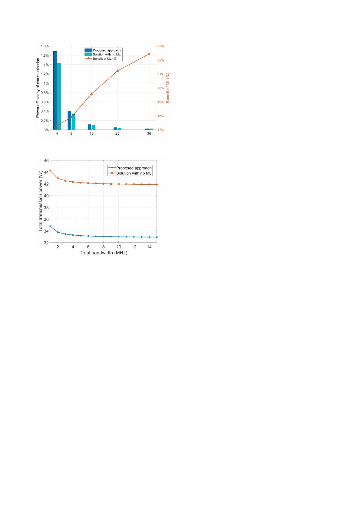
Machine Learning for Predicti v e On-Demand Deployment of U A Vs for W ireless Communications Qianqian Zhang 1 , Mohammad Mozaf fari 1 , W alid Saad 1 , Mehdi Bennis 2 , and M ´ erouane Debbah 3 , 4 1 Bradley Department of Electrical and Computer Engineering, V irginia T ech, V A, USA, Emails: { qqz93, mmozaff, w alids } @vt.edu. 2 Center for W ireless Communications, University of Oulu, Finland, Email: bennis@ee.oulu.fi. 3 Mathematical and Algorithmic Sciences Lab, Huawei France R&D, Paris, France, Email: merouane.debbah@huawei.com. 4 Large Systems and Networks Group, CentraleSup ´ elec, Universit ´ e Paris-Saclay , 3 rue Joliot-Curie, 91192 Gif-sur-Yvette, France. Abstract —In this paper , a novel machine learning (ML) framework is proposed for enabling a pr edictive, efficient deployment of unmanned aerial vehicles (U A Vs), acting as aerial base stations (BSs), to provide on-demand wireless service to cellular users. In order to hav e a comprehensi ve analysis of cellular traffic, an ML framework based on a Gaussian mixture model (GMM) and a weighted expectation maximiza- tion (WEM) algorithm is intr oduced to predict the potential network congestion. Then, the optimal deployment of U A Vs is studied to minimize the transmit power needed to satisfy the communication demand of users in the downlink, while also minimizing the power needed for U A V mobility , based on the predicted cellular traffic. T o this end, first, the optimal partition of service areas of each U A V is derived, based on a fairness principle. Next, the optimal location of each U A V that minimizes the total power consumption is derived. Simulation results show that the proposed ML approach can reduce the required downlink transmit power and improv e the power efficiency by over 20% , compared with an optimal deployment of U A Vs with no ML prediction. I . I N T RO D U C T I O N The demand for cellular data is experiencing an unprece- dented increase. The next generation, 5 G wireless cellular network is estimated to support a 200 fold increase in wireless data traffic by 2030 [1]. T o cope with this exponential in- crease in demand, there has been gro wing interest in network densification for cellular systems as a means to improv e spectrum efficiency and cellular network capacity [2]. The need for additional base stations (BSs) is more pro- nounced in cellular hotspot areas that exhibit a steep surge in data demands during temporary events, such as concerts and football games. T o satisfy such temporary surges in traf fic, the use of an unmanned aerial vehicle (UA V) as an aerial BS can be a more fle xible and cost-ef fecti ve approach, compared with a traditional, ground BS [3]. A mobile UA V can intelligently change its position, which is suitable to provide on-demand wireless service to ground users, thus o vercoming coverage holes and alleviating congestions [4]. In order to deploy U A Vs in a timely and flexible manner , network operators must be able to predict potential hotspots and congestion e vents a priori. T o this end, there is a need to apply machine learning (ML) techniques to analyze demand patterns [5]. The ability of ML to exploit big data analytics enables a comprehensiv e prediction of a network’ s traffic amount and data distrib ution. By using such predictions, aerial UA V BSs can be optimally deployed to the target area beforehand thus pro viding an on-demand, delay-free and power -efficient wireless service to ground users. The use of U A Vs as cellular BSs has been addressed in [4], [6]–[10]. Meanwhile, in [4] and [7], the authors studied the use of UA Vs as flying BSs to provide energy-ef ficient service to wireless users. Moreover , the work in [8] and [9] focus on using U A Vs as relays, and the work in [10] studies an energy-ef ficient trajectory design. Howe ver , most of the existing works assume a time-in variant wireless network, or a gi ven distribution of cellular users. T o properly analyze an on-demand deployment of UA V BSs, the temporal and spatial patterns of the cellular traffic data must be predicted so as to optimally deploy UA Vs to satisfy a time-varying data demand. There are existing woks, such as [9], [11], and [12], that apply ML techniques to optimize UA V deployment. In [9], a neural model is formulated to study the map of U A Vs to each hotspot areas. The authors in [11] studied the trajectory optimization using neural networks, while a segmented regression approach is proposed in [12] for U A V channel modeling, based on the terrain topology . Howe ver , none of these works demonstrates the benefit of applying ML to deploy U A Vs on-demand and improve po wer efficienc y and network performance. In order to analyze the data traffic of cellular networks, the authors in [13] studied a BS sleeping strategy for minimizing po wer consumption. Howe ver , the authors focused only on a low-traf fic cellular network, which is not scalable for the more practical, congested scenarios. The main contribution of this paper is a novel machine learning framework that enables operators to predict conges- tions and hotspot e vents, and subsequently , deploy temporary U A V BSs to provide aerial wireless service to mobile users, while minimizing the U A V po wer needed for do wnlink communications and mobility . W e consider a heterogeneous cellular network, in which ground BSs can of fload the wireless service to aerial UA Vs when the predicted data demand of mobile users exceeds the network capacity . T o guarantee a no-delay wireless service, a Gaussian mixture model (GMM) is introduced based on a weighted expectation maximization (WEM) algorithm [14] to predict the cellular data traffic. Then, the optimal deployment of U A Vs is studied to minimize the power needed for U A V transmission and mobility , giv en the predicted traf fic. T o this end, we first study the di vision of service areas, based on a fairness principle. Then, we deriv e the optimal U A V locations that can minimize the total power consumption of the network. T o the best of our knowledge, this is the first work that lev erages ML to predictiv ely deploy U A Vs as aerial BSs. Simulation results show that the proposed approach can reduce the required downlink transmit po wer and improve the po wer ef ficiency by ov er 20% , compared with an optimal deployment of UA Vs with no ML prediction. The rest of this paper is org anized as follows. Section II presents the system model and problem formulation. Section III outlines the proposed ML and U A V deployment frame- work. Simulation results are presented in Section IV, while conclusions are drawn in Section V. I I . S Y S T E M M O D E L A N D P RO B L E M F O R M U L AT I O N Consider a time-v ariant heterogeneous cellular network that serves a group of cellular users distributed in a geo- graphical area A . The cellular network consists of a set I of I U A Vs and a set J of J BSs. Each user can recei ve data from both ground BSs and UA Vs. Initially , a traditional BS will be chosen to serv e the wireless users. Ho wever , if the downlink of the ground cellular system is overloaded due to heavy traffic, the ground BS will request the deployment of U A V BSs to offload some of its users. Ground BSs and UA Vs employ different frequency bands for do wnlink communications. Each U A V is equipped with directional antennas that enable beamforming. Therefore, interference among U A Vs is negligible. Furthermore, each U A V adopts a frequency division multiple access (FDMA) technique and assigns a dedicated channel to one of its downlink users. Hereinafter , we use the notion of an aerial cell to indicate the service area of each U A V , and aerial cellular users to indicate users that are served by UA V cellular BSs. Each U A V has a limited energy resource, that must be efficiently used for joint communications and mobility . T o this end, the UA Vs should intelligently change their positions to meet the required users’ data rates, as well as to minimize their transmission po wer . Ho wev er, gi ven the cellular network is time-variant, the cellular traffic demand will change o ver time, which complicates the efficient deployment. T o guaran- tee timely aerial service without having U A Vs continuously moving, the network operator can use ML techniques to predict its network’ s data demand, and then, request the deployment of U A V BSs to the predicted hotspot areas, before the congestion occurs. A. Air-to-gr ound channel model Giv en a typical ground receiv er located at ( x, y ) ∈ A and a U A V i ∈ I located at ( x i , y i , h i ) , the path loss of the downlink communication from U A V i to the receiv er will be [15]: L i ( x, y )[ dB ] = 20 log  4 π f c d i ( x, y ) c  + ξ i , (1) where d i ( x, y ) = p ( x − x i ) 2 + ( y − y i ) 2 + h 2 i is the dis- tance between the ground receiver and UA V i , f c is the carrier frequency , c is the speed of light, and ξ i is the av erage additional loss to the free space propagation loss which depends on the en vironment. If the wireless link between U A V i and a ground user is line-of-sight (LOS), ξ LOS i ∼ N ( µ LOS , σ 2 LOS ) ; otherwise, the non-line-of-sight (NLOS) link has an additional loss of ξ NLOS i ∼ N ( µ NLOS , σ 2 NLOS ) . The NLOS link will experience a high path loss due to shadowing and reflection. The probability of existence of LOS links between UA V i and the ground user will then be [15]: p LOS i ( x, y ) = 1 1 + a exp  − b [ 180 π θ i ( x, y ) − a ]  , (2) where a and b are constant values which depend on the en vi- ronment, and θ i ( x, y ) = sin − 1 ( h i d i ( x,y ) ) is the ele vation angle of U A V i with respect to the receiver . Then, the probability of having a NLOS link is p NLOS i ( x, y ) = 1 − p LOS i ( x, y ) [4]. Consequently , the av erage path loss from U A V i to the ground reciever at ( x, y ) in the linear scale can be giv en as ¯ L i ( x, y ) = p LOS i ( x, y ) L LOS i ( x, y ) + p NLOS i ( x, y ) L NLOS i ( x, y ) . (3) Therefore, the downlink capacity that U A V i can provide to a mobile user located at ( x, y ) will be: R i ( x, y ) = W i log 2  1 + P i ( x, y ) G i ( x, y ) / ¯ L i ( x, y ) W i n 0  , (4) where W i is the transmission bandwidth of U A V i , P i ( x, y ) is the transmission po wer , G i ( x, y ) is the antenna gain of U A V i , and n o is the average noise power spectral density . For tractability , we assume a perfect beam alignment between the U A V and the mobile receiver , and each UA V has the same antenna gain. Therefore, G i ( x, y ) = G , which is a constant for all i ∈ I and ( x, y ) ∈ A . Assume that the total av ailable bandwidth of U A V i is B i and the number of mobile users associated with UA V i is N i , then the do wnlink bandwidth of each channel will be W i = B i / N i . The number N i of aerial users that are served by U A V i within its aerial cell is given by: N i = N Z Z A i f ( x, y ) d x d y , (5) where N = P i ∈I N i is the total number of aerial users, A i is the service area of U A V i , and f ( x, y ) is the distribution of aerial users. In order to provide a univ ersal wireless service, the aerial cells of all U A Vs should fully cover the geographical area A without overlap. That is, ∪ i ∈I A i = A , and for i 6 = j and i, j ∈ I , A i ∩ A j = ∅ . Howe ver , note that, the value of N and the user distribution f ( x, y ) will change, according to the offloading requests from ground BSs. B. Cellular traf fic analysis T o provide an on-demand service, network operators need to change the U A Vs’ locations frequently , according to the offload requests from ground BSs, to satisfy the instant traffic demand. Howe ver , such continuous movement will consume excessi ve po wer . T o ef ficiently deploy UA Vs while guaran- teeing a no-delay wireless service, a dataset of the cellular traffic history can be exploited by the network operator for traffic prediction. This dataset, represented by a matrix Q , records discrete data during each time period T for M days: Q = [ N ( x, y , t ) , D ( x, y , t ) |∀ t ∈ T , ( x, y ) ∈ A ] , (6) where T = { T , 2 T , · · · , 24 M } is a discrete set of time, and the unit of T is hour . The first item N ( x, y , t ) represents the number of aerial users that are offloaded from a BS at ( x, y ) to a U A V during a time interval from t to t + T , and the second item D ( x, y , t ) denotes the amount of cellular traf fic that a U A V needs to provide for the aerial users from a BS at ( x, y ) during the period from t to t + T . Let N be the total number of aerial users, D be the total amount of aerial cellular traf fic, f ( x, y ) be the spatial distri- butions of aerial users, and g ( x, y ) be the spatial distribution of aerial data traffic in A . Without a comprehensi ve analysis of Q , the values of N , D , f ( x, y ) and g ( x, y ) will change ov er time, based on the offloading requests of ground BSs, which causes a frequent movement of U A Vs to meet the instant traffic demand, and excessi ve power consumed on mobility . Therefore, our goal is to dev elop a centralized ML ap- proach to predict N and f ( x, y ) based on N ( x, y , t ) , and D and g ( x, y ) based on D ( x, y , t ) , such that at the beginning of each period T , network operators can optimally deploy U A Vs to minimize the power consumptions, while during each interval the locations of U A Vs remain fixed. C. Data rate r equir ement Giv en the predicted information on the total amount of aerial cellular traffic D , and the distribution of aerial cellular traffic g ( x, y ) , the av erage data rate requirement within a service area A i of UA V i can be giv en by α i = 1 T Z Z A i D · g ( x, y ) d x d y . (7) Since the communication capacity of U A V i should be greater than or equal to the rate demand of all users in its aerial cell A i , we formulate the data rate requirement as follows, Z Z A i R i ( x, y ) d x d y ≥ α i , (8) i.e., R i ( x, y ) ≥ D g ( x, y ) T . (9) W e define β ( x, y ) = Dg ( x,y ) T as the a verage minimum data rate requirement for the aerial user at ( x, y ) . Based on (4) and (9), the minimum transmit power that UA V i should provide to communicate with the user at ( x, y ) will be: P min i ( x, y ) = B i n 0 ¯ L i ( x, y ) GN i  2 β ( x,y ) N i /B i − 1  . (10) Note that, the values of N i and β ( x, y ) in (10) will depend on the output of the cellular traffic analysis. Consequently , the total transmit po wer of all U A Vs needed to satisfy the data demand of all aerial users in A will be: P c = X i ∈I Z Z A i P min i ( x, y ) d x d y . (11) W ithout loss of generality , we assume that the maximum transmission power of U A Vs is sufficient to meet the data demand of aerial users. Meanwhile, the total power for each U A V i ∈ I to move from its current location ( x o i , y o i , h o i ) to the new location ( x i , y i , h i ) will be: P t = γ X i ∈I  ( x o i − x i ) 2 + ( y o i − y i ) 2 + ( h o i − h i ) 2  1 2 , (12) where γ is the rate of energy consumption a UA V needs to mov e by one meter . Then, the second objective is to jointly find the optimal location and the partition of the service area A i for each U A V i ∈ I , such that the total po wer used for downlink transmissions and mobility can be minimized, i.e., min A i ,x i ,y i ,h i P c + P t , (13a) s. t. R R A i P min i ( x, y ) d x d y P a i = κ, ∀ i ∈ I , (13b) ∪ i ∈I A i = A , (13c) A i ∩ A j = ∅ , ∀ i 6 = j ∈ I , (13d) where P a i is the a vailable po wer of U A V i , and κ is a constant for all i ∈ I . The first constraint represents a fairness principle, whereby the ratio of the data traffic of floaded to each UA V equals to the ratio of the av ailable power of each U A V . The second and third constraints guarantee that the service areas of all U A Vs fully cover A without ov erlap. Note that, without an ML analysis, the function P min i , as well as P c , will change, based on the offloading requests of ground BSs. Thus, the network operator needs to reorganize the aerial cellular system to meet the instant traffic demand frequently . Howe ver , with the predicted information of cel- lular traffic, the optimal problem (13) is fixed within each period T . Therefore, at the beginning of each interval, U A Vs are deployed according to the solution of (13), and within the period, the location and aerial cell of each UA V remain unchanged. I I I . P RO P O S E D P R E D I C T I O N A N D UA V D E P L O Y M E N T F R A M E W O R K Next, we propose a novel approach to address the afore- mentioned problems. First, a centralized ML approach will be proposed to predict the v alues of N , D , f ( x, y ) and g ( x, y ) for each time interval T . With the prediction information, the power minimization problem in (13) will be solved to optimally deploy each U A V . A. Cellular traf fic prediction In order to hav e a robust and practical analysis, we use the real dataset 1 of City Cellular T raf fic Map [16], which records 1 Our approach can accommodate other datasets without loss of generality . the time, the location of each BS, the number of mobile users, and the total amount of data that each BS serves during each hour , from Aug. 19 to Aug. 26, 2012, in a median-size city in China. W e assume that the maximum number of mobile users that each BS can serve within one hour is a fixed number of N m , and the maximum amount of cellular data is a constant D m for all BSs. Thus, a ne w dataset is gen- erated to capture the traffic of the aerial cellular network as Q 0 = [ N ( x, y , t ) − N m , D ( x, y , t ) − D m |∀ t ∈ T , ( x, y ) ∈ A ] , in which N ( x, y , t ) − N m is the number of aerial users from hour t to t + 1 , and D ( x, y , t ) − D m is the amount of aerial cellular traffic. For notation simplicity , hereinafter, we use Q to denote the aerial traf fic dataset, instead of Q 0 . Since N ( x, y , t ) and D ( x, y , t ) have an analogous data structure, a similar approach will be applied to analyze N ( x, y , t ) and D ( x, y , t ) . For simplicity , we keep the following discussion only on D ( x, y , t ) . Therefore, the objectiv e is to use ML to formulate the temporal and spatial pattern of D ( x, y , t ) . There are three key assumptions in the following ML analysis. First, due to the periodicity of human acti vity , the cellular traffic presents a repetitiv e daily pattern [17]. Based on this observ ation, we assume that the total cellular traffic during a specific hour of dif ferent days follows the same distribution. Therefore, we divide the dataset into 24 subsets, by mer ging the data of the same hour from different days. Second, we assume that the traffic amount between each hour of one day is independent. Therefore, given the 24 sub- datasets, 24 independent models will be built to study the pattern of each objectiv e value of each hour . Furthermore, we assume that the temporal feature of D ( x, y , t ) is independent from the spatial distribution. As a result, two separate models will be studied to identify the temporal feature D ( t ) and the spatial feature g ( x, y ) of D ( x, y , t ) for each hour . The model to capture the temporal and spatial charac- teristics of D ( x, y , t ) relies on a GMM, which assumes that the data distribution can be modeled by the sum of multiple Gaussians with different weights as [18] p ( x ) = P K k =1 π k N ( x | µ k , Σ k ) , where x is a general data point, p ( x ) is the probability distributed at x , K is the number of individual Gaussian models in GMM, and P K k =1 π k = 1 , π k ∈ [0 , 1] is the mixing coefficient for each Gaussian. 1) Spatial distribution model: First, we study the mod- eling approach of the spatial feature g ( x, y ) of D ( x, y , t ) . Giv en a time t ∈ { 1 , 2 , · · · , 24 } , the data distribution of the cellular traffic from t to t + 1 can be calculated by g t ( x, y ) = D ( x, y , t ) R R A D ( x, y , t ) d x d y . (14) Then, a dataset G t is formed by all the distribution g t ( x, y ) of M days for the specific hour t , and we seek to b uild a GMM to capture a pattern of data distribution for time t as g t ( x ) = K t X k =1 π t k N ( x | µ t k , Σ t k ) , (15) where x = ( x, y ) is the location vector . T o find the parame- ters of K t , π t k , µ t k , and Σ t k , for a giv en t ∈ { 1 , 2 , · · · , 24 } , Algorithm 1 Proposed algorithm to find parameters of the spatial distribution model g t ( x, y ) Input : G t for a giv en t Output : { π k } , { µ k } and { Σ k } , for each k ∈ { 1 , · · · , K } Part I : W eighted K-means for parameter initialization Input : G t Output : K , { µ k } k ∈{ 1 , 2 , ··· ,K } A. For K = K min : K max 1. Randomly choose K initial values of { µ k } k ∈{ 1 , ··· ,K } , 2. Loop : a. Calculate the weighted distance of each data point to each µ k by D ( x, y , t ) | x − µ k | , b . Assign each data point x to cluster k ∗ , such that k ∗ = arg min k D ( x, y , t ) | x − µ k | , c. Recalculate µ k by averaging the v alues of data points belonging to cluster k as µ k = P C k D ( x, y , t ) x / P C k D ( x, y , t ) , d. Check con ver gence: if { µ k } k ∈{ 1 , 2 , ··· ,K } changes. B. Choose the value of K that minimizes the ratio of intra-cluster to inter- cluster distance [18]. Part II : W eighted EM iteration Input : G t , K , { µ k } k ∈{ 1 , 2 , ··· ,K } Output : { π k } , { µ k } and { Σ k } , for each k ∈ { 1 , · · · , K } 1. Initialize Σ k to be an identical matrix, and π k = 1 /K . 2. E step : Calculate the posterior probability for each data point x n belonging to each cluster k by r nk = π k N ( x n | µ k , Σ k ) / P K i =1 π i N ( x n | µ i , Σ i ) , 3. M step : Recalculate the parameters using the posterior probability r nk a. µ k = P N n =1 D ( x, y , t ) r nk x n / N k b . Σ k = P N n =1 D ( x, y , t ) r nk ( x n − µ k )( x n − µ k ) T / N k c. π k = N k /K where N k = P N n =1 D ( x, y , t ) r nk . 4. Check the conver gence by (16). If not conv erged, return to E step. and k ∈ { 1 , · · · , K t } , first, a classification approach based on a weighted K-means method is used to group the data x into K clusters, and the weight D ( x, y , t ) is the data amount at x = ( x, y ) . Then, the WEM algorithm will be used to find the optimal parameters of GMM. The con vergence of the WEM iterativ e approach can be ev aluated by the log likelihood function as ln L ( Σ , µ , π ) = X n ln X k π k D ( x n ) g t ( x n | Σ k , µ k ) , (16) whose v alue will increase as the iteration time increases. Our detailed approach is summarized in Algorithm 1. 2) T emporal distribution model: Giv en a time t , the total aerial traffic amount in the system from t to t + 1 can be calculated by D t = P ( x,y ) ∈A D ( x, y , t ) . By gathering the data D t of M days, we have a dataset D t = { D t 1 , · · · , D t M } . The GMM that captures the temporal pattern of D t is p ( D t ) = P V t v =1 π t v N ( D t | µ t v , Σ t v ) . The approach to model the temporal distribution D t for D ( x, y , t ) , is similar to the algorithm in Algorithm 1. Howe ver , both the K-means and EM algorithm do not add weight to each data point. As a result, by ignoring all D ( x, y , t ) used in T able 1 and substituting its value by one, Algorithm 1 can be applied to find the temporal pattern D t . The mixture Gaussian model p ( D t ) is a probability density function (pdf) over the cellular data amount, from which we can get the cumulative distribution function (CDF) as C t ( d ) = R d −∞ p ( D t ) d D t . The predicted data amount can be estimated by the CDF with a threshold. For example, with a threshold of 60% , the predicted traffic amount ov er the aerial networks can be given by D t = C − 1 t (0 . 6) . The ML analysis of the temporal feature N ( t ) and the spatial feature f ( x, y ) of N ( x, y , t ) can follow the approach of Algorithm 1. B. On-demand, optimal UA V deployment In order to optimally deploy UA Vs to minimize the total power , problem (13) is formulated, which jointly considers the aerial cell partition and the U A Vs’ locations. With the prediction information, network operators only need to mov e U A Vs at the beginning of each time interv al, according to the solution of (13). Howe ver , solving (13) is challenging due to the mutual dependence between ( x i , y i , h i ) and A i with N i and β ( x, y ) . For tractability , we solve (13) in two sequential steps. First, gi ven the current location of each U A V i ∈ I , we seek to find the optimal partition of the service area A i for each U A V , that minimizes the power for transmissions. Then, for each UA V i , gi ven its fixed service area A i , the optimal location is deri ved to minimize the required po wer for downlink communications and mobility . 1) Optimal partition of service ar eas: Given the current location of each U A V i ∈ I , we aim to find the best partition of service areas {A i } i ∈I , such that the total power for downlink communications of all UA Vs is minimized. The optimal partition problem can be formulated as follows, min A i P c , (17a) s. t. Z Z A i P min i ( x, y ) d x d y = κP a i , ∀ i ∈ I , (17b) ∪ i ∈I A i = A , (17c) A i ∩ A j = ∅ , ∀ i 6 = j ∈ I . (17d) T o solve this problem, we use our previously developed gradient-based method in [19, Theorem 1, Algorithm 1]. 2) Optimal locations: Gi ven the optimal partition of the service area {A i } i ∈I , the power minimization problem can be reduced into I subproblems for each U A V i ∈ I as min x i ,y i ,h i P c i + P t i . (18) Based on [4, Theorem 1], we focus on two scenarios in the following discussions. One is a high-altitude U A V , where h 2 i  ( x − x i ) 2 + ( y − y i ) 2 , and the other is the low-altitude U A V , where h 2 i  ( x − x i ) 2 + ( y − y i ) 2 . In scenario one, the value of θ i in (2) is approximately 90 ◦ , thus, p LOS i ( x, y ) ≈ 1 and ¯ L i ( x, y ) ≈ L LOS i ( x, y ) . Then, P i can be rewritten as P c i ≈ O i Z Z A i Z i ( x, y )  d 2 i ( x, y ) + 10 0 . 1 ξ LOS i  d x d y , (19) where O i =  4 π f c c  2 B i n 0 GN i is a coefficient that does not depend on ( x, y ) , and Z i ( x, y ) = 2 β ( x,y ) N i /B i − 1 . It is obvious that P i is a con ve x function with respect to x i and y i . By setting the first partial deriv ativ es to be zero, we have the Fig. 1: T otal and av erage required power for data transmission. optimal locations for U A V i that minimize the transmission power P c i as x ∗ i = R R A i x Z i ( x, y ) d x d y R R A i Z i ( x, y ) d x d y , (20a) y ∗ i = R R A i y Z i ( x, y ) d x d y R R A i Z i ( x, y ) d x d y . (20b) Although the objective function P c i + P t i is con ve x with respect to x i and y i , deriving a closed-form solution of (18), which minimizes both the transmit and mobility po wer for each U A V , is challenging. Howe ver , it is easy to find the optimal solution of (18) based on a gradient-based algorithm. Using a similar approach, we can find the optimal location for scenario two. I V . S I M U L A T I O N R E S U LT S A N D A NA LY S I S For simulations, we consider a U A V cellular network operating in a 5 GHz frequency band for downlink commu- nications. The total av ailable bandwidth for each U A V is 10 MHz. The noise power spectral is set to − 174 dBm/Hz. For each U A V , the antenna gain is 10 dB, and the rate of energy consumption for moving per meter is γ = 0 . 1 Joules per meter . For ML, we use 7 8 of the dataset to train the model, and the remaining 1 8 data is used to e valuate the performance. Fig. 1 shows the total and average communication power per U A V required to satisfy the users’ data demands for two scenarios: the proposed approach and a solution with no ML predictions. In each case, the proposed optimal partition of service areas and the optimal location deployment are employed. Fig. 1 shows that, as the number of U A Vs increases, both the total required po wer and the average communication power will decrease. When more U A Vs are av ailable, each aerial BS can serve a smaller cov erage area, yielding a lo wer av erage path loss. Therefore, the needed total transmit power decreases, giv en a fixed amount of the total cellular traf fic. As the total required transmit power decreases, the average power reduces accordingly . Fig. 1 further shows that compared with the solution without ML predictions, the Fig. 2: A verage power ef ficiency of U A V wireless communications ov er total power consumption. Fig. 3: Required transmit power as a function of the total band- width. proposed approach yields a significant improvement of power consumptions. The po wer reduction v aries from 20 . 68% to 24 . 40% , as the number of UA Vs increases from 9 to 36 . Fig. 2 shows the power ef ficiency , defined as the average percentage of the transmit power P c out of total power P c + P t . As the number of U A Vs increases, the power efficiencies in both scenarios will decrease. Here, we note that U A V mobility will often require more power than wireless transmission. By deploying more UA Vs, network operator is more likely to send a UA V to meet an instant communication in a relatively far hotspot area, which causes more po wer consumed for mobility . Also, as shown in Fig. 1, more U A Vs requires using a less communication power P c , which further reduces the power efficiency . Moreover , Fig. 2 shows that compared with the solution without ML, the proposed method can improv e the power efficiency of U A V communication by up to 22 . 34% . Fig. 3 shows the required transmit power as a function of the total bandwidth, assuming nine UA Vs. As the a vailable bandwidth increases, the transmit power will decrease. How- ev er, a wider bandwidth results in a higher noise power , which prev ents the reduction of transmit power , especially when the bandwidth is greater than 5 MHz. For such noise-sensiti ve system, a lower spectrum ef ficiency cannot sav e additional power . V . C O N C L U S I O N In this paper , we have proposed a novel approach for predictiv e deployment of U A V aerial BSs to provide an on-demand wireless service to the cellular users. W e hav e formulated a power minimization problem to optimize the partition of the service area of each U A V , while minimizing the U A V power needed for downlink communications and mobility . In order to predict hotspots, a nov el ML framew ork based on GMM and WEM has been dev eloped. The results hav e sho wn that the proposed ML approach can reduce the required downlink transmit power , and improve the av erage power efficiency by over 20% , compared with an optimal deployment of U A Vs with no ML prediction. R E F E R E N C E S [1] S. Rangan, T . S. Rappaport, and E. Erkip, “Millimeter-wav e cellular wireless networks: Potentials and challenges, ” Pr oceedings of the IEEE , vol. 102, no. 3, pp. 366–385, Feb 2014. [2] N. Bhushan, J. Li, D. Malladi, R. Gilmore, D. Brenner, A. Damn- janovic, R. Sukhavasi, C. Patel, and S. Geirhofer, “Network densi- fication: the dominant theme for wireless evolution into 5G, ” IEEE Communications Magazine , v ol. 52, no. 2, pp. 82–89, Feb 2014. [3] M. Mozaffari, W . Saad, M. Bennis, Y .-H. Nam, and M. Debbah, “ A tutorial on U A Vs for wireless networks: Applications, challenges, and open problems, ” arXiv preprint , 2018. [4] M. Mozaffari, W . Saad, M. Bennis, and M. Debbah, “Optimal transport theory for power-ef ficient deployment of unmanned aerial vehicles, ” in Pr oc. of IEEE International Conference on Communications (ICC) , Kuala Lumpur, Malaysia, May 2016, pp. 1–6. [5] M. Chen, U. Challita, W . Saad, C. Y in, and M. Debbah, “Machine learning for wireless networks with artificial intelligence: A tutorial on neural networks, ” arXiv preprint , 2017. [6] M. Mozaffari, W . Saad, M. Bennis, and M. Debbah, “Efficient de- ployment of multiple unmanned aerial vehicles for optimal wireless coverage, ” IEEE Communications Letters , vol. 20, no. 8, pp. 1647– 1650, Jun 2016. [7] Z. Becvar , M. V ondra, P . Mach, J. Plachy , and D. Gesbert, “Per- formance of mobile networks with U A Vs: Can flying base stations substitute ultra-dense small cells?” in Pr oc. of 23th European W ireless Confer ence , Dresden, Germany , May 2017, pp. 1–7. [8] K. Li, W . Ni, X. W ang, R. P . Liu, S. S. Kanhere, and S. Jha, “Energy- efficient cooperati ve relaying for unmanned aerial vehicles, ” IEEE T ransactions on Mobile Computing , vol. 15, no. 6, pp. 1377–1386, Aug 2016. [9] V . Sharma, M. Bennis, and R. Kumar , “U A V-assisted heterogeneous networks for capacity enhancement, ” IEEE Communications Letters , vol. 20, no. 6, pp. 1207–1210, 2016. [10] Y . Zeng and R. Zhang, “Energy-efficient U A V communication with tra- jectory optimization, ” IEEE T ransactions on W ir eless Communications , vol. 16, no. 6, pp. 3747–3760, Mar 2017. [11] J. F . Horn, E. M. Schmidt, B. R. Geiger , and M. P . DeAngelo, “Neural network-based trajectory optimization for unmanned aerial vehicles, ” Journal of Guidance, Control, and Dynamics , vol. 35, no. 2, pp. 548– 562, Mar-Apr 2012. [12] J. Chen, U. Y atnalli, and D. Gesbert, “Learning radio maps for UA V- aided wireless networks: A segmented regression approach, ” in Pr oc. of IEEE International Conference on Communications (ICC) , Paris, France, July 2017, pp. 1–6. [13] S. Zhang, S. Zhao, M. Y uan, J. Zeng, J. Y ao, M. R. L yu, and I. King, “T raffic prediction based power saving in cellular networks: A machine learning method, ” in Proc. of the 25th ACM SIGSP ATIAL International Confer ence on Advances in Geographic Information Systems , Redondo Beach, CA, USA, Nov 2017, p. 29. [14] I. D. Gebru, X. Alameda-Pineda, F . Forbes, and R. Horaud, “EM algorithms for weighted-data clustering with application to audio-visual scene analysis, ” IEEE T ransactions on P attern Analysis and Machine Intelligence , vol. 38, no. 12, pp. 2402–2415, Jan 2016. [15] A. Al-Hourani, S. Kandeepan, and S. Lardner, “Optimal LAP alti- tude for maximum coverage, ” IEEE W ireless Communications Letters , vol. 3, no. 6, pp. 569–572, July 2014. [16] “City cellular traf fic map, ” https://github .com/caesar0301/ city- cellular- traf fic- map, accessed: 2016-10-05. [17] U. Paul, A. P . Subramanian, M. M. Buddhikot, and S. R. Das, “Under - standing traffic dynamics in cellular data networks, ” in Pr oc. of IEEE International Confer ence on Computer Communications (INFOCOM) , Shanghai, China, Apr 2011, pp. 882–890. [18] M. B. Christopher, P attern recognition and mac hine learning . Springer-V erlag Ne w Y ork, 2016. [19] M. Mozaffari, W . Saad, M. Bennis, and M. Debbah, “Wireless com- munication using unmanned aerial vehicles (UA Vs): Optimal transport theory for hover time optimization, ” IEEE T ransactions on W ir eless Communications , vol. 16, no. 12, pp. 8052–8066, Apr 2017.