Multi-Class Management with Sub-Class Service for Autonomous Electric Mobility On-Demand Systems

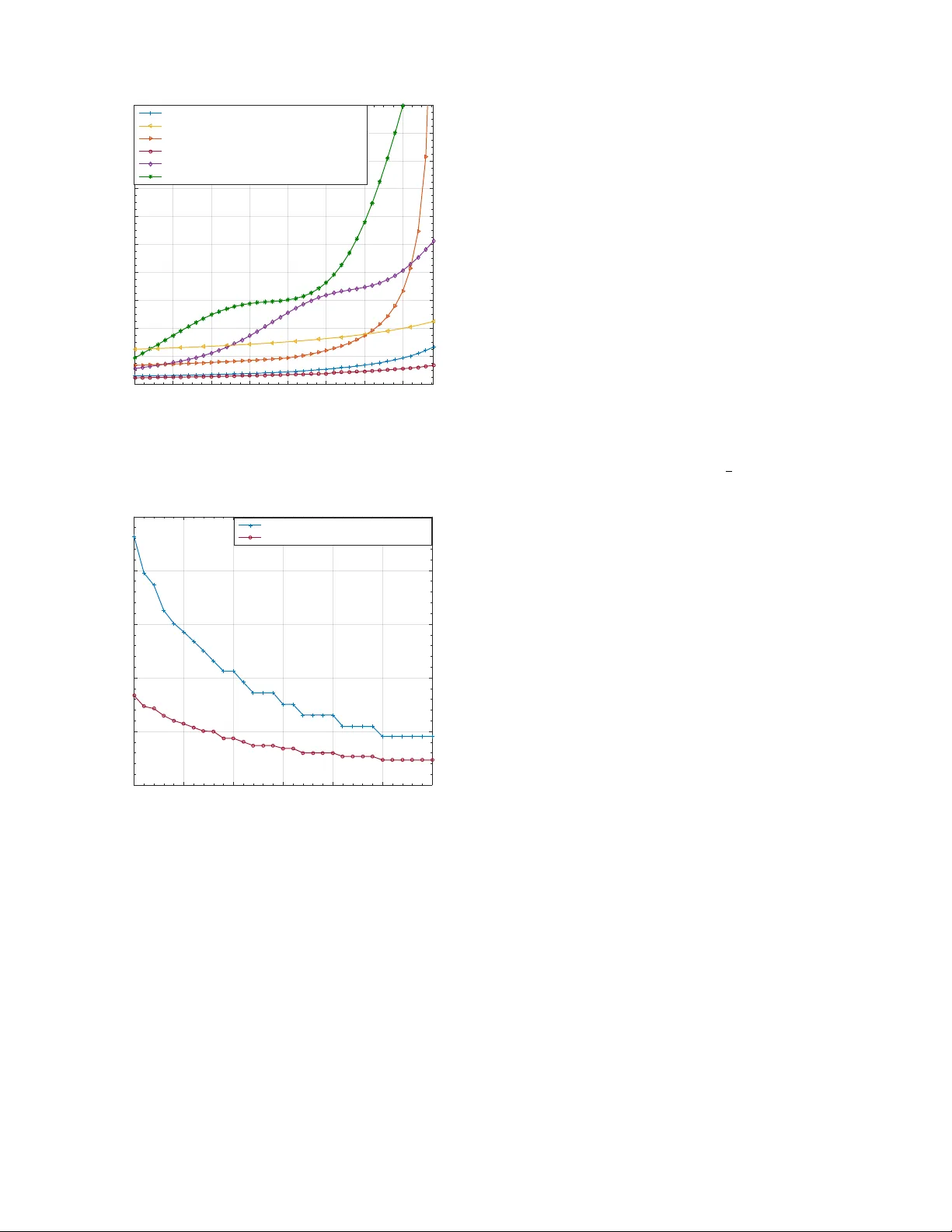
1 Multi-Class Management with Sub-Class Service for Autonomous Electric Mobility On-Demand Systems Syrine Belakaria ∗ , Mustafa Ammous ∗ , Sameh Sorour ∗ and Ahmed Abdel-Rahim † ‡ ∗ Department of Electrical and Computer Engineering, Uni versity of Idaho, Mosco w , ID, USA † Department of Ci vil and En vironmental Engineering, Uni v ersity of Idaho, Mosco w , ID, USA ‡ National Institute for Adv anced T ransportation T echnologies, Uni versity of Idaho, Mosco w , ID, USA Email: { bela7898, ammo1375 } @v andals.uidaho.edu, { samehsorour , ahmed } @uidaho.edu Abstract —Despite the significant advances in vehicle automa- tion and electrification, the next-decade aspirations for massive deployments of autonomous electric mobility on demand (AE- MoD) services are still thr eatened by two major bottlenecks, namely the computational and charging delays. This paper proposes a solution for these two challenges by suggesting the use of fog computing for AEMoD systems, and developing an optimized char ging scheme for its vehicles with and multi- class dispatching scheme f or the customers. A queuing model repr esenting the proposed multi-class management scheme with sub-class service is first introduced. The stability conditions of the system in a given city zone are then derived. Decisions on the proportions of each class v ehicles to partially/fully charge, or directly ser ve customers of possible sub-classes ar e then optimized in order to minimize the maximum response time of the system. Results show the merits of our optimized model compared to a pre viously proposed scheme and other non-optimized policies. Keyw ords — A utonomous Mobility On-Demand; Electric V ehicle; F og-based Architecture; Dispatching; Charging; Queuing Systems. I . I N T RO D U C T I O N Urban transportation systems are facing tremendous chal- lenges nowadays due to the dominant dependency and mas- siv e increases on priv ate vehicle ownership, which result in dramatic increases in road congestion, parking demand [1], [2], and carbon footprint [3] [4]. These challenges can be mitigated with the significant advances of vehicle electrifica- tion, automation, and connectivity . W ith more than 10 million self-driving cars expected to be on the road by 2025 [5], it is forecasted that vehicle ownership will significantly decline by 2025, as it will be replaced by the nov el concept of Autonomous Electric Mobility on-Demand (AEMoD) services [6], [7]. In such system, customers will simply need to press some b uttons on an app to promptly get an autonomous electric vehicle transporting them door-to-door , with no pick-up/drop- off and driving responsibilities, no dedicated parking needs, no vehicle insurance and maintenance costs, and extra in- vehicle leisure times. W ith these qualities, AEMoD systems will succeed in attracting millions of subscribers and providing This study was supported by the Pacific Northwest Univ ersity Transporta- tion center (Pac trans) project KLK864. The authors would like to thank all who contribute to this study from both funding agencies. hassle-free pri v ate urban mobility . Despite the great aspirations for wide AEMoD service deployments by early-to-mid next decade, the timeliness (and thus success) of such service is threatened by two major bottle- necks. First, the expected massive demand of AEMoD services will result in excessi ve if not prohibitive computational and communication delays if cloud based approaches are employed for the micro-operation of such systems. Moreover , the typical full-battery charging rates of electric vehicles will not be able to cope with the gigantic numbers of vehicles in volv ed in these systems, thus resulting in instabilities and unbounded customer delays. Several recent works Recent works have addressed important problems in AMoD systems by building dif ferent operation models for them like a distributed spatially av eraged queuing model and a lumped Jackson network model [9] also the system was [13] cast into a closed multi-class BCMP queuing network to solve the routing problem on congested roads. Many key factors were not considered in these works in order to simplify the mathematical resolution. None of these papers considered the computational architecture for massiv e demands on such services, the vehicle electrification, and the influence of char ging limitations on its stability . In [18] [19] we proposed a closely related model management model for Amods Systems. W e proposed to resolve the first limitation, communication/computation delays, by suggesting the exploitation of the new and trendy fog-based networking and computing ar chitectur es [20]. The privile ges brought by this technique [18], will allow handling instantaneous decision making applications such as AEMoD system operations in a distributed and accelerated way . The fog controller in each service zone is responsible of collecting information about customer requests, vehicle in-flow to the service zone, their state-of-charge (SoC), and the av ailable full-battery charging rates in the service zone. Giv en the collected information, it can promptly make dispatching, and charging decisions for these vehicles in a timely manner . In order to solve the second problem, we proposed previ- ously [18], [19] that the fog controller will smartly cope with the av ailable charging capabilities of each service zone, by assigning to each customer a vehicle that has enough charge to serve him without in route charging. In the former solution, arriving vehicles in each service zone are subdivided into different classes in ascending order of their SoC corresponding 2 to the different customer classes. Different proportions of each class vehicles will either wait (without charging) for dispatching to its corresponding customer class or partially charge to serve a customer from the same class. V ehicles arriving with depleted batteries will be allo wed to either partially or fully charge. Despite the valuable results given by this model but the dispatching process of the system can result on having all the vehicles depleted by the end of the service which may cause the instability of the system. In this paper we keep the same charging scheme and we propose an enhanced dispatching process that allow each vehicle to serve all the sub-classes of customers (customers that needs lower state of char ge) The question now is: T o maintain char ging stability and minimize the maximum r esponse time of the system, What ar e the optimal Charging and sub-classes dispatching deci- sions? T o address this question, a queuing model representing the proposed multi-class management with sub-class service scheme is first introduced. The stability conditions of this model. Decisions on the proportions of each class vehicles to partially/fully charge, or directly serve customers and decision on which class will be served are then optimized. Finally , the merits of our proposed optimized decision scheme are tested and compared to several non optimized schemes. I I . S Y S T E M M O D E L W e consider one service zone controlled by a fog controller connected to: (1) the service request apps of customers in the zone; (2) the AEMoD v ehicles; (3) C rapid char ging points dis- tributed in the service zone and designed for short-term partial charging; and (4) one spacious rapid charging station designed for long-term full charging. AEMoD vehicles enter the service in this zone after dropping off their latest customers in it. Their detection as free vehicles by the zone’ s controller can thus be modeled as a Poisson process with rate λ v . Customers request service from the system according to a Poisson process. Both customers and vehicles are classified into n classes based on an ascending order of their required trip distance and the corresponding SoC to cover this distance, respectively . From the thinning property of Poisson processes, the arri v al process of Class i customers and vehicles, i ∈ { 0 , . . . , n } , are both independent Poisson processes with rates λ ( i ) c and λ v p i , where p i is the probability that the SoC of an arriving vehicle to the system belongs to Class i . Note that p 0 is the probability that a vehicle arrive with a depleted battery , and is thus not able to serve immediately . Consequently , λ (0) c = 0 as no customer will request a vehicle that cannot trav el any distance. On the other hand, p n is also equal to 0, because no vehicle can arriv e to the system fully charged as it has just finished a prior trip. Upon arriv al, each vehicle of Class i , i ∈ { 1 , . . . , n − 1 } , will park anywhere in the zone until it is called by the fog controller to either: (1) join vehicles that will serve customer with their current state of charge with probability q i (The served customer can be from any Sub-class j with j ≤ i ); or (2) partially charge up to the SoC of class i + 1 at any of the C charging points (whenev er any of them becomes free), with probability q i = 1 − q i , before parking again in waiting Fig. 1. Joint dispatching and partially/fully charging model, abstracting an AEMoD system in one service zone. to serve a customer from any Sub-class j with j ≤ i + 1 . As for Class 0 vehicles that are incapable of serving before charging, they will be directed to either fully charge at the central charging station with probability q 0 , or partially charge at one of C charging points with probability q 0 = 1 − q 0 . In the former and latter cases, the vehicle after charging will wait to serve customers of any Sub-class j ≤ n and 1 , respectiv ely . Considering the abov e explanation, Each vehicle, whether decided to serve immediately or decided to charge before serving, will be able to serve: (1) customers from same class with probability Π ii ; or (2) customers with a trip distance from any Sub-class with probability Π ij . As widely used in the literature (e.g., [12], [13]), the full charging time of a vehicle with a depleted battery is assumed to be exponentially distributed with rate µ c . Given uniform SoC quantization among the n vehicle classes, the partial charging time can then be modeled as an exponential random v ariable with rate nµ c . Note that the larger rate of the partial charging process is not due to a speed-up in the charging process but rather due to the reduced time of partially charging. The customers belonging to Class i , arriving at rate λ ( i ) c , will be served at a rate of λ ( i ) v s , which includes summation of proportions of arriv al rates of vehicles that: (1) arri ved to the zone with a SoC belonging to Class j ∀ j ≥ i and were directed to wait to serve Class i ∀ i ≤ j customers; or (2) arrived to the zone with a SoC belonging to Class j − 1 and were directed to partially charge to be able to serve a Sub-Class i ∀ i ≤ j customers. Giv en the abov e description and modeling of variables, the entire zone dynamics can thus be modeled by the queuing system . This system includes n M/M/1 queues for the n classes of customer service, one M/M/1 queue for the central charging station, and one M/M/C queue representing the partial char ging process at the C charging points. Assuming that the service zones will be designed to guaran- tee a maximum time for a vehicle to reach a customer, our goal in this paper is to minimize the maximum expected response time of the entire system. By response time, we mean the time needed that vehicle starts moving from its parking or charging spot to wards this customer . 3 I I I . S Y S T E M S TA B I L I T Y C O N D I T I O N S In this section, we first deduce the stability conditions of our proposed joint dispatching and charging system, using the basic laws of queuing theory . Each class of vehicles with an arriv al rate λ ( i ) v will be characterized by its SoC when it is ready to serve customers. Each of the n classes of customers are served by a separate queue of vehicles, with λ ( i ) v s being the arriv al rate of the vehicles that are av ailable to serve the customers of the i th class. Consequently , it is the service rate of the customers i th arriv al queues. W e can thus deduce from the system model in the previous section the rate of vehicles with SoC that allows to serve a class i or any sub-class j ≤ i that requires lo wer SoC to serve its customers: λ ( i ) v = λ v ( p i − 1 q i − 1 + p i q i ) , i = 1 , . . . , n − 1 . λ ( n ) v = λ v ( p n − 1 q n − 1 + p 0 q 0 ) (1) Since we know that q i + q i = 1 Then we substitute q i by 1 − q i in order to have a system with n v ariables λ ( i ) v = λ v ( p i − 1 − p i − 1 q i − 1 + p i q i ) , i = 1 , . . . , n − 1 λ ( n ) v = λ v ( p n − 1 − p n − 1 q n − 1 + p 0 q 0 ) (2) W e can also deduce the expression of the rate of vehicles that will actually serve a class of customers i : λ ( i ) v s = n X k = i λ ( k ) v Π ki , i = 1 , . . . , n (3) By injecting the expression of λ k v in (2) in (3), we find: λ ( i ) v s = λ v n − 1 X k = i ( p k − 1 − p k − 1 q k − 1 + p k q k )Π ki + λ v ( p n − 1 − p n − 1 q n − 1 + p 0 q 0 )Π ni , i = 1 , . . . , n − 1 λ ( n ) v s = λ v ( p n − 1 − p n − 1 q n − 1 + p 0 q 0 )Π nn (4) From the well-kno wn stability condition of an M/M/1 queue: λ ( i ) v s > λ ( i ) c , i = 1 , . . . , n (5) T o guarantee customers’ satisfaction, the fog controller of each zone must impose an av erage response time limit T for any class. W e can thus express this av erage response time constraint for the customers of the i -th class as: 1 λ ( i ) v s − λ ( i ) c ≤ T or λ ( i ) v s − λ ( i ) c ≥ R , with R = 1 T (6) Before reaching the customer service queues, the vehicles will go through a decision step of either to go to these queues immediately or partially charge. From the system model, we hav e the following stability constraints on the C char ging points and central charging station queues, respectively: n − 1 X i =0 λ v ( p i − p i q i ) < C ( nµ c ) λ v p 0 q 0 < µ c (7) The following lemma allows the estimation of the average needed vehicles arriv al for a giv en service zone. Lemma 1: For the entire zone stability , and fulfillment of the average response time limit for all its classes, the av erage vehicles arriv al rate must be lower bounded by: λ v ≥ n X i =1 λ ( i ) c + nR (8) Pr oof: The proof of Lemma 1 is in Appendix A of [11]. I V . J O I N T C H A R G I N G A N D D I S PA T C H I N G O P T I M I Z A T I O N A. Pr oblem F ormulation The goal of this paper is to minimize the maximum e xpected response time of the system’ s classes. The response time of any class is defined as the average of the duration from any customer request until a vehicle is dispatched to serve him/her . The maximum expected response time is expressed as: max i ∈{ 1 ,...,n }  1 λ ( i ) v s − λ ( i ) c  (9) It is obvious that the system’ s class having the maximum expected response time is the one that hav e the minimum expected response rate. In other words, we have: arg max i ∈{ 1 ,...,n }  1 λ ( i ) v s − λ ( i ) c  = arg min i ∈{ 1 ,...,n } n λ ( i ) v s − λ ( i ) c o (10) Consequently , minimizing the maximum expected response time is equiv alent to maximizing the minimum expected re- sponse rate. Using the epigraph form [14] of the latter problem, we get the following stochastic optimization problem: maximize q 0 ,...,q n − 1 , Π 11 ,..., Π nn R (11a) s.t λ v n − 1 X k = i ( p k − 1 − p k − 1 q k − 1 + p k q k )Π ki (11b) + λ v ( p n − 1 − p n − 1 q n − 1 + p 0 q 0 )Π ni − λ ( i ) c ≥ R (11c) i = 1 , . . . , n − 1 (11d) λ v ( p n − 1 − p n − 1 q n − 1 + p 0 q 0 )Π nn − λ ( n ) c ≥ R (11e) n − 1 X i =0 λ v ( p i − p i q i ) < C ( nµ c ) (11f) λ v p 0 q 0 < µ c (11g) i X j =1 Π ij = 1 , i = 1 , . . . , n (11h) 0 ≤ Π ij ≤ 1 , i = 1 , . . . , n, j = 1 , . . . , i (11i) 0 ≤ q i ≤ 1 , i = 0 , . . . , n − 1 (11j) n − 1 X i =0 p i = 1 , 0 ≤ p i ≤ 1 , i = 0 , . . . , n − 1 (11k) 0 < R ≤ λ v − P n i =1 λ ( i ) c n (11l) (11m) 4 The n constraints in (11d) and (11e) represent the epigraph form’ s constraints on the original objecti ve function in the right hand side of (10), after separation [14] and substituting ev ery λ ( i ) v s by its expansion form in (4). The constraints in (11f) and (11g) represent the stability conditions on charging queues. The constraints in (11h), (11i),(11j) and (11k) are the axiomatic constraints on the probabilities (i.e., v alues being between 0 and 1, and sum equal to 1). The Finally , Constraint (11l) is a positivity constraint on the minimum expected response rate. Finally , Constraint (11l) is is a positivity constraint and the upper bound on R introduced by Lemma (1). B. Lower Bound Analytical Solutions The optimization problem in (11) is a quadratic non-con ve x problem with second order dif ferentiable objecti ve and con- straint functions. Usually , the solution obtained by using the Lagrangian and KKT analysis for such non-con vex problems provides a lower bound on the actual optimal solution. Con- sequently , we propose to solve the above problem by first finding the solution deriv ed through Lagrangian and KKT analysis, then, if needed, iterativ ely tightening this solution to the feasibility set of the original problem. The Lagrangian function associated with the optimization problem in (11) is giv en by the following expression: L ( R, q , Π , α , β , γ , ω , µ , ν , δ ) = − n − 1 X i =0 ω i q i − ω n ( R −  2 ) + n − 1 X i =1 α i [ λ ( i ) c − λ v n − 1 X k = i ( p k − 1 − p k − 1 q k − 1 + p k q k )Π ki − λ v ( p n − 1 − p n − 1 q n − 1 + p 0 q 0 )Π ni + R ] + α n ( λ ( n ) c − λ v ( p n − 1 − p n − 1 q n − 1 + p 0 q 0 )Π ni + R ) + β 0 ( n − 1 X i =0 λ v ( p i − p i q i ) − C ( nµ c )) + β 1 ( λ v p 0 q 0 − µ c ) + n − 1 X i =0 γ i ( q i − 1) + γ n ( R − λ v − P n i =1 λ ( i ) c n ) − R + n X i =1 i X j =1 ν ij (Π ij − 1) − µ ij Π ij + n X i =1 δ i ( i X k =1 Π ik − 1) (12) where: • q = [ q 0 , . . . , q n − 1 ] is the vector of charing decisions. • Π = [Π ij ] is the vector of dispatching decisions to serve customers. • α = [ α i ] , such that α i is the associated Lagrange multiplier to the i -th customer queues inequality . • β = [ β i ] , such that β i is the associated Lagrange multiplier to the i -th charging queues inequality . • δ = [ δ i ] , such that δ i is the associated Lagrange mul- tiplier to the i -th equality constraint on the dispatching decision. • γ = [ γ i ] , such that γ i is the associated Lagrange multiplier to the i -th upper bound inequality on the charging decisions and the expected response time. • ω = [ ω i ] , such that ω i is the associated Lagrange multiplier to the i -th lower bound inequality on the charging decisions and the expected response time. • µ = [ µ ij ] , such that µ ij is the associated Lagrange multiplier to the j -th lower bound inequality on the dispatching decision Π ij . • ν = [ ν ij ] , such that ν ij is the associated Lagrange multiplier to the j -th upper bound inequality on the dispatching decision Π ij . For more accurate resolutions, Three small positive constants  0 ,  1 and  2 are added to the stability conditions on the charging queues and the positivity condition on the maximum expected waiting time to make them non strict inequalities. Solving the equations gi ven by the KKT conditions on the problem equality and inequality constraints, the following theorem illustrates the optimal lower bound solutions of the problem in (11). Theor em 1: The lower bound solution of the optimization problem in (11), obtained from Lagrangian and KKT analysis can be expressed as follows: where ζ i and ζ ij are the solution that that maximize inf q , Π L ( q , Π ∗ , R ∗ , α ∗ , β ∗ , γ ∗ , ω ∗ , µ ∗ , ν ∗ , δ ∗ ) Pr oof: The proof of Theorem 1 is in Appendix C in [11]. C. Solution T ightening As stated earlier, the closed-form solution deriv ed in the previous section from analyzing the constraints’ KKT con- ditions does not always match with the optimal solution of the original optimization problem, and is sometimes a non- feasible lo wer bound on our problem. Unfortunately , there is no method to find the exact closed-from solution of non- con vex optimization. Howe ver , starting from the deriv ed lower bound, we can numerically tighten this solution by iterating tow ard the feasible set of the original problem. There are sev eral algorithms to iterativ ely tighten lower bound solutions, one of which is the Sugg est-and-Impr ove algorithm algorithm proposed in [17] to tighten non-con ve x quadratic problems. W e will thus propose to employ this method whenev er the KKT conditions based solution is not feasible and tightening is required. V . S I M U L A T I O N R E S U LT S In this section, we test the merits of our proposed scheme using extensi ve simulations. The metric used to ev aluate these merits is the maximum expected response times of the different classes. For all the performed simulation figures, the full- charging rate of a vehicle is set to µ c = 0 . 033 mins − 1 , and the number of charging points C = 40 . Fig. 2 depicts the maximum expected response time for different values of P n i =1 λ ( i ) c , while fixing λ v to 8 min − 1 . For this setting, n = 7 is the smallest number of classes that satisfy the stability condition in Lemma 2 in [18]. From queuing theory rules [15] [16] the more serving queues a system have, 5 R ∗ =          λ v − P n i =1 λ ( i ) c n γ ∗ n 6 = 0  2 ω ∗ n 6 = 0 P n − 1 i =1 α ∗ i ( λ v P n − 1 k = i ( p k − 1 − p k − 1 q ∗ k − 1 + p k q ∗ k )Π ∗ ki + λ v ( p n − 1 − p n − 1 q ∗ n − 1 + p 0 q ∗ 0 )Π ∗ ni − λ ( i ) c ) + α ∗ n ( λ v ( p n − 1 − p n − 1 q ∗ n − 1 + p 0 q ∗ 0 )Π ∗ nn − λ ( n ) c ) O ther w ise q ∗ 0 =                0 α ∗ 1 Π ∗ 11 − P n i =1 α ∗ i Π ∗ ni − β ∗ 0 + β ∗ 1 > 0 1 α ∗ 1 Π ∗ 11 − P n i =1 α ∗ i Π ∗ ni − β ∗ 0 + β ∗ 1 < 0 λ ( n ) c + λ v p n − 1 q ∗ n − 1 Π ∗ nn − λ v p n − 1 Π ∗ nn + R ∗ λ v p 0 Π nn ∗ α ∗ n 6 = 0 µ c λ ∗ v p 0 β ∗ 1 6 = 0 ζ 0 ( R ∗ , q ∗ , Π ∗ , α ∗ , β ∗ , γ ∗ , ω ∗ , µ ∗ , ν ∗ , δ ∗ ) O ther w ise q ∗ i =          0 α ∗ i +1 − α ∗ i − β ∗ 0 > 0 1 α ∗ i +1 − α ∗ i − β ∗ 0 < 0 i = 1 , . . . , n − 1 . R ∗ + λ ( i ) c + λ v [ P n − 1 k = i +2 ( p k − 1 q ∗ k − 1 − p k q ∗ k )Π ki +( p n − 1 q ∗ n − 1 − p 0 q ∗ 0 )Π ni − P n k = i p k − 1 Π ki + p i − 1 q ∗ i − 1 Π ∗ ii − p i +1 q i +1 Π i +1 i +1 ] λ v p i (Π ii − Π i +1 i +1 ) α ∗ i 6 = 0 ζ i ( R ∗ , q ∗ , Π ∗ , α ∗ , β ∗ , γ ∗ , ω ∗ , µ ∗ , ν ∗ , δ ∗ ) O ther w ise Π ∗ ij =    0 α ∗ j λ v ( p i − 1 q i − 1 ∗ − p i − 1 − p i q ∗ i ) + δ ∗ i > 0 1 α ∗ j λ v ( p i − 1 q i − 1 ∗ − p i − 1 − p i q ∗ i ) + δ ∗ i < 0 ζ ij ( R ∗ , q ∗ , Π ∗ , α ∗ , β ∗ , γ ∗ , ω ∗ , µ ∗ , ν ∗ , δ ∗ ) O ther w ise i = 1 , . . . , n − 1 . (13) the higher the waiting time will be. Moreover , in pre vious related work [18] [19], we showed that increasing the number of classes n beyond its strict lo wer bound introduced in Lemma 2 in [18] will damage the system performance and increase the maximum response time. Fig. 2 compare the maximum expected response time per- formances against P n i =1 λ ( i ) c , for different decision approaches namely our deriv ed optimal decisions to the following deci- sions sets: 1) Optimized charging decisions (i.e. q i ∀ i ) with same class dispatching (i.e. Π ii = 1 ∀ i and Π ij = 0 ∀ i, j 6 = i ) 2) Always partially charge decisions (i.e. q i = 0 ∀ i ) with same class dispatching (i.e. Π ii = 1 ∀ i and Π ij = 0 ∀ i, j 6 = i ) 3) Equal split charging decisions (i.e. q i = 0 . 5 ∀ i ) with same class dispatching (i.e. Π ii = 1 ∀ i and Π ij = 0 ∀ i, j 6 = i ) 4) Always partially charge decisions (i.e. q i = 0 ∀ i ) with proportional sub-classes dispatching decisions (i.e. Π ij proportional to the customers sub-classes needs) 5) Equal split charge decisions (i.e. q i = 0 ∀ i ) with proportional sub-classes dispatching decisions (i.e. Π ij proportional to the customers sub-classes needs) These fiv e schemes represent the possible non-optimized policies, in which each vehicle takes its own fixed decision irrespectiv e of the system parameters. These schemes are possible in case of a non connected and optimized system. Fig. 2 compares these approaches with a decreasing SoC distribution. The figure clearly sho w superior performances for our deriv ed optimal policy compared to the other policies, especially as P n i =1 λ ( i ) c gets closer to λ v , which are the most properly engineers scenarios (as large differences between these two quantities results in very low utilization), This approv es the expression found in lemma 1. A Gains of 49.3%, 69.8%, 93.22%, 86.7% and 94.4% in the performances, can be noticed compared to the previously stated policies respectiv ely . Fig. 3 shows the study of the resilience requirements for our considered model in the critical scenarios of sudden reduction in the number of charging sources within the zone. This reduction may occur due to either natural (e.g., typical failures of one or more stations) or intentional (e.g., a malicious attack on the fog controller blocking its access to these sources). The resilience measure that the fog controller can take in these scenarios is to notify its customers of a transient increase in the vehicles’ response times giv en the av ailable vehicles in the zone. For this, we are only comparing the ne w proposed model to our previously proposed model. The figures shows clearly the advantage brought by the sub-class dispatching model. The gain gets higher in critical scenarios and reaches up to 65% with very acceptable maximum response time e ven is very low energy resources. This demonstrates the importance of our proposed scheme in achieving better customer satisfaction. V I . C O N C L U S I O N In this paper , we proposed solutions to the computational and charging bottlenecks threatening the success of AEMoD systems. The computational bottleneck can be resolved by employing a fog-based architecture to distrib ute the optimiza- tion loads ov er different service zones, reduce communication delays, and matches the nature of dispatching and charging processes of AEMoD vehicles. W e also proposed a multi- class dispatching and charging scheme and dev eloped its 6 2 2.5 3 3.5 4 4.5 5 5.5 Total Arrival Rate of the Customers ' 1 n 6 c i 0 5 10 15 20 25 30 35 40 45 50 Maximum Expected Response Time (min) Total Arrival Rate of the Vehicles 6 v = 8 Optimized charge/same class dispatch Always charge/same class dispatch Equal split charge/same class dispatch Optimized charge and sub-class dispatch Always Charge/proportional sub-class dispatch Equal split charge/proportional sub-class dispatch Fig. 2. Comparison to non-optimized policies for Decreasing SoC distribu- tion. 10 15 20 25 30 35 40 Available charging stations C 0 5 10 15 20 25 Maximum Expected Response Time (min) 6 v =8, ' 1 n 6 c i =5 Optimized charge/same class dispatch Optimized charge and sub-class dispatch Fig. 3. Effect of varying charging points availability . queuing model and stability conditions. W e then formulated the problem of optimizing the proportions of vehicles of each class that will partially/fully charge or directly serve customers of same class or any lower sub-class as an optimization problem, in order to minimize the maximum expected system response time while respecting the system stability constraints. The opti- mal decisions and corresponding maximum response time were analytically derived. Simulation results demonstrated both the merits of our proposed optimal decision scheme compared to typical non-optimized schemes and previously optimized scheme, and its performance for dif ferent distributions of vehicle SoC and customer trip distances. R E F E R E N C E S [1] W . J. Mitchell, C. E. Borroni-Bird, and L. D. Burns, “Reinventing the Automobile: Personal Urban Mobility for the 21st Century”. Cambridge, MA: The MIT Press, 2010. [2] D. Schrank, B. Eisele, and T . Lomax, “TTIs 2012 Urban Mobility Report, ” T exas A&M T ransportation Institute , T exas, USA.2012. [3] U. N. E. Programme, “The Emissions Gap Report 2013 - UNEP , ” T ech. Rep. , 2013. [4] U. E. P . Agency , “Greenhouse Gas Equiv alencies Calculator, ” T ech.Rep. , 2014. [Online]: http://www .epa.gov/cleanener gy/energy- resources/refs.html [5] “IoT And Smart Cars: Changing The W orld For The Better , ” Digitalist Magazine , August 30, 2016. [Online]: http://www .digitalistmag.com/iot/2016/08/30/iot-smart-connected- cars-willchange-world-04422640 [6] “T ransportation Outlook: 2025 to 2050, ” Navigant Resear ch, Q216 , 2016. [Online]: http://www .navigantresearch.com/research/transportation- outlook-2025-to-2050. [7] “The Future Is Now: Smart Cars And IoT In Cities, ” F orbes , June 13, 2016. [Online]: http://www .forbes.com/sites/pikeresearch/2016/06/13/the-future-is- now-smartcars/63c0a25248c9 [8] “Fog Computing and the Internet of Things: Extend the Cloud to Where the Things Are, ” Cisco White P aper , 2015. [Online]:http://www .cisco.com/c/dam/en us/solutions/trends/iot/docs/computing- overvie w .pdf [9] R. Zhang, K. Spieser, E. Frazzoli, and M. Pav one, “Models, Algorithms, and Evaluation for Autonomous Mobility-On-Demand Systems, ” in Pr oc. of American Control Conf. , Chicago, Illinois, 2015. [10] R. Zhang, F . Rossi, and M. Pa vone, “Model Predictive Control of Autonomous Mobility-on-Demand Systems, ” in Proc. IEEE Conf. on Robotics and Automation , Stockholm, Sweden, 2016. [11] S. Belakaria, M. Ammous, S. Sorour, and A. Abdel-Rahim, ”Multi- Class Management with Sub-Class Service for Autonomous Electric Mobility On-Demand Systems”,2018. [Online] https://arxiv .org [12] H. Liang, I. Sharma, W . Zhuang, and K. Bhattacharya,“Plug-in Electric V ehicle Charging Demand Estimation based on Queueing Network Analysis, ” IEEE P ower and Ener gy Society General Meeting , 2014. [13] K. Zhang, Y . Mao, S. Leng, Y . Zhang, S. Gjessing, and D.H.K. Tsang, “Platoon-based Electric V ehicles Charging with Renewable Energy Sup- ply: A Queuing Analytical Model, ” in Proc. of IEEE International Confer ence on Communications (ICC16) , 2016. [14] S. Boyd and L. V andenberghe, “Conve x Optimization”, 1st ed. Cam- bridge: Cambridge University Press , 2015. [15] A. Papoulis and S. Pillai, Probability , Random V ariables, and Stochastic Processes, 4th ed. International Edition: McGraw-Hill, 2002. [16] A.L. Garcia, Probability , Statistics, and Random Processes for Electrical Engineering, 3rd ed., Prentice Hall, 2008. [17] S. Boyd and J. Park, “General Heuristics for Nonconv ex Quadratically Constrained Quadratic Programming’. Stanford University , 2017. [18] S. Belakaria, M. Ammous, S. Sorour, and A. Abdel-Rahim, “ A Multi- Class Dispatching and Charging Scheme for Autonomous Electric Mo- bility On-Demand, ” IEEE 86th V ehicular T echnology Conference (VTC- F all) , 2017. [19] S. Belakaria, M. Ammous, S. Sorour , and A. Abdel-Rahim, “Optimal V ehicle Dimensioning for Multi-Class Autonomous Electric Mobility On-Demand Systems, ” IEEE International Communication Conference (ICC) , 2018. [20] Y . Mao, C. Y ou, J. Zhang, K. Huang, and K. B. Letaief, ”A Survey on Mobile Edge Computing: The Communication Perspective, ” IEEE com- munication surveys & tutorials, VOL. 19, NO. 4, FOURTH QUARTER, 2017. 7 A P P E N D I X A P R O O F O F L E M M A 1 From (4) and (6) we have : λ ( i ) c + R ≤ λ v n − 1 X k = i ( p k − 1 − p k − 1 q k − 1 + p k q k )Π ki + λ v ( p n − 1 − p n − 1 q n − 1 + p 0 q 0 )Π ni , i = 1 , . . . , n − 1 λ ( n ) c + R ≤ λ v ( p n − 1 − p n − 1 q n − 1 + p 0 q 0 )Π nn (14) The summation of all the inequalities in (14) giv es a new inequality n X i =1 λ ( i ) c + nR ≤ n X i =1 n X k =1 λ ( k ) v Π ki (15) Which is equi v alent to: n X i =1 λ ( i ) c + nR ≤ n X i =1 λ ( i ) v i X k =1 Π ik (16) Since W e hav e P i j =1 Π ij = 1 , i = 1 , . . . , n then: n X i =1 λ ( i ) c + nR ≤ n X i =1 λ ( i ) v (17) From (1) and (2) n X i =1 λ ( i ) v = n − 1 X i =1 ( p i − 1 q i − 1 + p i q i ) + ( p n − 1 q n − 1 + p 0 q 0 ) (18) Since q i + q i = 1 and we have P n − 1 i =0 p i = 1 then: n X i =1 λ ( i ) c + nR ≤ λ v (19) A P P E N D I X B P R O O F O F T H E O R E M 1 Applying the KKT conditions to the inequalities constraints of (11), we get: α ∗ i ( λ ( i ) c + R ∗ − λ v n − 1 X k = i ( p k − 1 − p k − 1 q ∗ k − 1 + p k q ∗ k )Π ∗ ki − λ v ( p n − 1 − p n − 1 q ∗ n − 1 + p 0 q ∗ 0 )Π ∗ ni ) = 0 i = 1 , . . . , n − 1 α ∗ n ( λ ( n ) c + R ∗ − λ v ( p n − 1 − p n − 1 q ∗ n − 1 + p 0 q ∗ 0 )Π ∗ nn ) = 0 . β ∗ 0 ( n − 1 X i =0 λ v ( p i − p i q ∗ i ) − C ( nµ c )) = 0 . β ∗ 1 ( λ v p 0 q ∗ 0 − µ c ) = 0 γ ∗ i ( q ∗ i − 1) = 0 , i = 0 , . . . , n − 1 . γ ∗ n ( R ∗ − λ v − P n i =1 λ ( i ) c n ) = 0 . ω ∗ i q ∗ i = 0 , i = 0 , . . . , n − 1 . ω ∗ n ( R ∗ −  2 ) = 0 . ν ∗ ij (Π ∗ ij − 1) = 0 , i = 1 , . . . , n, j = 1 , . . . i. µ ∗ ij Π ∗ ij = 0 , i = 1 , . . . , n, j = 1 , . . . i. δ ∗ i ( i X j =1 Π ∗ ij − 1) = 0 , i = 1 , . . . , n. (20) 8 Like wise, applying the KKT conditions to the Lagrangian function in (12), and kno wing that the gradient of the Lagrangian function goes to 0 at the lower bound solution, we get the follo wing set of equalities: ∂ L ∂ q i = λ v p i   i X j =1 α ∗ j (Π ∗ i +1 j − Π ∗ ij ) + α ∗ i +1 Π ∗ i +1 i +1 − β ∗ 0   − ω ∗ i + γ ∗ i = 0 , i = 1 , . . . , n − 1 . ∂ L ∂ q 0 = λ v p 0   α ∗ 1 Π ∗ 11 − n X j =1 α ∗ j Π ∗ nj − β ∗ 0 + β ∗ 1   − ω ∗ 0 + γ ∗ 0 = 0 ∂ L ∂ Π ij = α ∗ j λ v ( p i − 1 q i − 1 ∗ − p i − 1 − p i q ∗ i ) + δ ∗ i + ν ∗ ij − µ ∗ ij = 0 ∂ L ∂ Π nj = α ∗ j λ v ( p n − 1 q n − 1 ∗ − p n − 1 − p 0 q ∗ 0 ) + δ ∗ n + ν ∗ nj − µ ∗ nj = 0 ∂ L ∂ R = − 1 + n X i =1 α ∗ i − ω ∗ n + γ ∗ n = 0 (21) Multiplying the each of the partial deriv ati ves in (21) by the deri v ation variable itself combined with the KKT conditions of the variables lower bounds inequalities giv en by (20) giv es : ∂ L ∂ q i × q i = q ∗ i λ v p i   i X j =1 α ∗ j (Π ∗ i +1 j − Π ∗ ij ) + α ∗ i +1 Π ∗ i +1 i +1 − β ∗ 0   + γ ∗ i = 0 , i = 1 , . . . , n − 1 . ∂ L ∂ q 0 × q 0 = q ∗ 0 λ v p 0   α ∗ 1 Π ∗ 11 − n X j =1 α ∗ j Π ∗ nj − β ∗ 0 + β ∗ 1   + γ ∗ 0 = 0 ∂ L ∂ Π ij × Π ij = Π ∗ ij  α ∗ j λ v ( p i − 1 q i − 1 ∗ − p i − 1 − p i q ∗ i ) + δ ∗ i  + ν ∗ ij = 0 ∂ L ∂ Π nj × Π nj = Π ∗ nj  α ∗ j λ v ( p n − 1 q n − 1 ∗ − p n − 1 − p 0 q ∗ 0 ) + δ ∗ n  + ν ∗ nj = 0 ∂ L ∂ R × R = − R + R n X i =1 α ∗ i − ω ∗ n  2 + γ ∗ n ( λ v − P n i =1 λ ( i ) c n ) = 0 (22) When we inject the result of the first four equations in (22) in the KKT conditions on the upper bound conditions of the variables q i and Π ij we find: q ∗ i ( q ∗ i − 1)   i X j =1 α ∗ j (Π ∗ i +1 j − Π ∗ ij ) + α ∗ i +1 Π ∗ i +1 i +1 − β ∗ 0   = 0 , i = 1 , . . . , n − 1 . q ∗ 0 ( q ∗ 0 − 1)   α ∗ 1 Π ∗ 11 − n X j =1 α ∗ j Π ∗ nj − β ∗ 0 + β ∗ 1   = 0 Π ∗ ij (Π ∗ ij − 1)  α ∗ j λ v ( p i − 1 q i − 1 ∗ − p i − 1 − p i q ∗ i ) + δ ∗ i  = 0 Π ∗ nj (Π ∗ nj − 1)  α ∗ j λ v ( p n − 1 q n − 1 ∗ − p n − 1 − p 0 q ∗ 0 ) + δ ∗ n  = 0 (23) From (23) we have : 0 < q ∗ 0 < 1 only if α ∗ 1 Π ∗ 11 − P n j =1 α ∗ j Π ∗ nj − β ∗ 0 + β ∗ 1 = 0 0 < q ∗ i < 1 only if P i j =1 α ∗ j (Π ∗ i +1 j − Π ∗ ij ) + α ∗ i +1 Π ∗ i +1 i +1 − β ∗ 0 = 0 0 < Π ∗ ij < 1 only if α ∗ j λ v ( p i − 1 q i − 1 ∗ − p i − 1 − p i q ∗ i ) + δ ∗ i = 0 0 < Π ∗ nj < 1 only if α ∗ j λ v ( p n − 1 q n − 1 ∗ − p n − 1 − p 0 q ∗ 0 ) + δ ∗ n = 0 Since 0 ≤ q ∗ i ≤ 1 and 0 ≤ Π ∗ ij ≤ 1 then these equalities may not alw ays be true if α ∗ 1 Π ∗ 11 − P n j =1 α ∗ j Π ∗ nj − β ∗ 0 + β ∗ 1 > 0 and we know that γ ∗ 0 ≥ 0 then γ ∗ 0 = 0 which gi ves q ∗ 0 6 = 1 and q ∗ 0 = 0 . if P i j =1 α ∗ j (Π ∗ i +1 j − Π ∗ ij ) + α ∗ i +1 Π ∗ i +1 i +1 − β ∗ 0 > 0 which giv es q ∗ i 6 = 1 and q ∗ i = 0 9 if α ∗ 1 Π ∗ 11 − P n j =1 α ∗ j Π ∗ nj − β ∗ 0 + β ∗ 1 < 0 then γ ∗ 0 > 0 (it cannot be 0 because this will contradict with the v alue of q i ), which implies that q ∗ 0 = 1 . if P i j =1 α ∗ j (Π ∗ i +1 j − Π ∗ ij ) + α ∗ i +1 Π ∗ i +1 i +1 − β ∗ 0 < 0 then γ ∗ i > 0 (it cannot be 0 because this contradicts with the value of q i ), which implies that q ∗ i = 1 if α ∗ j λ v ( p i − 1 q i − 1 ∗ − p i − 1 − p i q ∗ i ) + δ ∗ i > 0 and we know that ν ∗ ij ≥ 0 then ν ∗ ij = 0 which gi ves Π ∗ ij 6 = 1 and Π ∗ ij = 0 . if α ∗ j λ v ( p n − 1 q n − 1 ∗ − p n − 1 − p 0 q ∗ 0 ) + δ ∗ n > 0 which giv es Π ∗ nj 6 = 1 and Π ∗ nj = 0 if α ∗ j λ v ( p i − 1 q i − 1 ∗ − p i − 1 − p i q ∗ i ) + δ ∗ i < 0 then ν ∗ ij > 0 (it cannot be 0 because this will contradict with the value of Π ij ), which implies that Π ij = 1 . if α ∗ j λ v ( p n − 1 q n − 1 ∗ − p n − 1 − p 0 q ∗ 0 ) + δ ∗ n < 0 then ν ∗ nj > 0 (it cannot be 0 because this will contradict with the v alue of Π nj ), which implies that Π nj = 1 . W e ha ve also from the KKT conditions given by equation in in (20) that says either the Lagrangian coef ficient is 0 or its the associated inequality is an equality: if β ∗ 1 6 = 0 we ha ve q ∗ 0 = µ c λ ∗ v p 0 if α ∗ n 6 = 0 we ha ve λ ( n ) c + λ v p n − 1 q ∗ n − 1 Π ∗ nn − λ v p n − 1 Π ∗ nn + R ∗ λ v p 0 Π nn ∗ if α ∗ i 6 = 0 , we hav e q ∗ i = R ∗ + λ ( i ) c + λ v [ P n − 1 k = i +2 ( p k − 1 q ∗ k − 1 − p k q ∗ k )Π ki +( p n − 1 q ∗ n − 1 − p 0 q ∗ 0 )Π ni − P n k = i p k − 1 Π ki + p i − 1 q ∗ i − 1 Π ∗ ii − p i +1 q i +1 Π i +1 i +1 ] λ v p i (Π ii − Π i +1 i +1 ) for i = 1 , . . . , n − 1 Otherwise by the Lagrangian relaxation: q ∗ i = ζ i ( R ∗ , q ∗ , Π ∗ , α ∗ , β ∗ , γ ∗ , ω ∗ , µ ∗ , ν ∗ , δ ∗ ) for i = 1 , . . . , n − 1 and Π ∗ ij = ζ ij ( R ∗ , q ∗ , Π ∗ , α ∗ , β ∗ , γ ∗ , ω ∗ , µ ∗ , ν ∗ , δ ∗ ) where ζ i and ζ ij are the solution that that maximize inf q , Π L ( q , Π ∗ , R ∗ , α ∗ , β ∗ , γ ∗ , ω ∗ , µ ∗ , ν ∗ , δ ∗ ) Now in order to find the expression of R ∗ we first look at its upper bound associated condition in (20). From there we can say that if ω ∗ n 6 = 0 then R ∗ =  2 and if γ ∗ n 6 = 0 then R ∗ = λ v − P n i =1 λ ( i ) c n Otherwise, from the last equation in (22), if ω ∗ n = 0 and γ ∗ n = 0 then R ∗ = n − 1 X i =1 α ∗ i ( λ v n − 1 X k = i ( p k − 1 − p k − 1 q ∗ k − 1 + p k q ∗ k )Π ∗ ki + λ v ( p n − 1 − p n − 1 q ∗ n − 1 + p 0 q ∗ 0 )Π ∗ ni − λ ( i ) c ) + α ∗ n ( λ v ( p n − 1 − p n − 1 q ∗ n − 1 + p 0 q ∗ 0 )Π ∗ nn − λ ( n ) c ) (24)