Fast 3D Point Cloud Denoising via Bipartite Graph Approximation & Total Variation

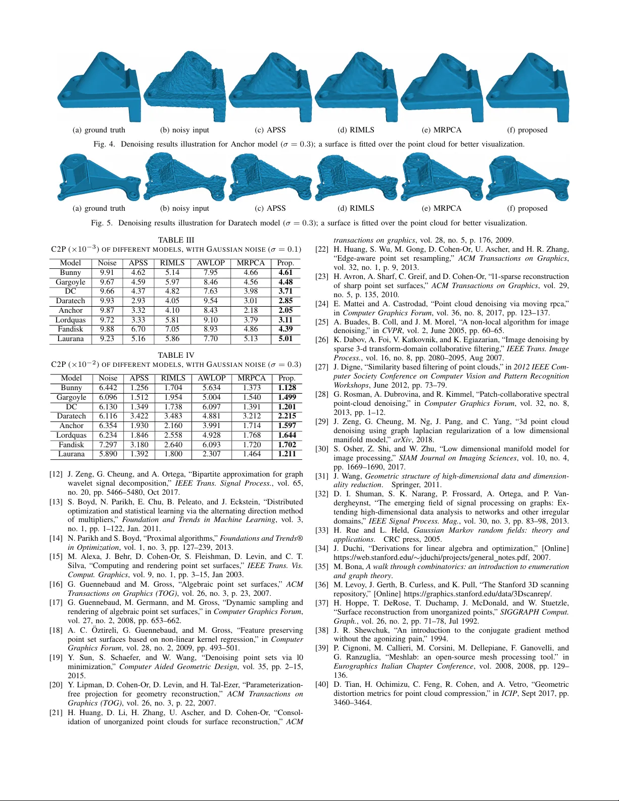
F ast 3D Point Cloud Denoising via Bipartite Graph Approximation & T otal V ariation Chinthaka Dinesh #1 , Gene Cheung ? 2 , Iv an V . Baji ´ c #3 , Cheng Y ang ? 4 # Simon F r aser University , Burnaby , BC, Canada; ? National Institute of Informatics, T okyo, J apan 1 hchintha@sfu.ca; 2 cheung@nii.ac.jp; 3 ibajic@ensc.sfu.ca; 4 cheng@nii.ac.jp Abstract —Acquired 3D point cloud data, whether from active sensors directly or from stereo-matching algorithms indir ectly , typically contain non-negligible noise. T o address the point cloud denoising problem, we propose a fast graph-based local algorithm. Specifically , given a k -nearest-neighbor graph of the 3D points, we first approximate it with a bipartite graph (independent sets of red and blue nodes) using a KL diver gence criterion. For each partite of nodes (say red), we first define surface normal of each red node using 3D coordinates of neighboring blue nodes, so that red node normals n can be written as a linear function of red node coordinates p . W e then formulate a con vex optimization problem, with a quadratic fidelity term k p − q k 2 2 given noisy observed red coordinates q and a graph total variation (GTV) regularization term f or surface normals of neighboring red nodes. W e minimize the resulting l 2 - l 1 -norm using alternating dir ection method of multipliers (ADMM) and proximal gradient descent. The two partites of nodes are alternately optimized until con vergence. Experimental results show that compared to state-of-the-art schemes with similar complexity , our proposed algorithm achieves the best overall denoising performance objectively and subjectively . Index T erms —graph signal processing, point cloud denoising, total variation, bipartite graph appr oximation I . I N T RO D U C T I O N Point cloud is no w a popular representation of 3D visual data in signal processing, and there are ongoing efforts in standardization bodies such as MPEG 1 and JPEG-PLENO 2 to efficiently compress the data. Point cloud can be acquired directly using acti ve sensors like Microsoft Kinect cameras, or computed indirectly from multiple vie wpoint images using e x- isting stereo-matching algorithms [1]. In either case, acquired point cloud data tend to be noisy , and thus denoising should be performed prior to compression. W e address the point cloud denoising problem in this paper . T ypically , an in verse problem like image super-resolution or deblurring [2] is ill-posed and requires a suitable regularization term to formulate a mathematically rigorous optimization problem. Because point cloud data are irregularly sampled in 3D space, typical signal priors like total variation (TV) [3] cannot be directly used. While graph variant of TV (called GTV) has been proposed [4], [5], applying GTV directly on the 3D point coordinates, as done in [6], is not appropriate, because GTV of coordinates promotes v ariational proximity of 3D points, and only a singular 3D point cloud has zero GTV value. 1 https://mpeg.chiariglione.or g/standards/mpeg-i/point-cloud-compression. 2 https://jpeg.or g/jpegpleno/pointcloud.html. In this paper , we argue that GTV is more appropriately applied to the surface normals of the 3D point cloud, so that GTV promotes smooth object surfaces lik e a tabletop—a generalization of functional smoothness in con ventional TV to 3D geometry . While there exist numerous methods to compute surface normals of 3D point clouds [7]–[11], the computations are typically nonlinear , resulting in difficult optimizations. T o alleviate this problem, we propose to first partition the 3D point cloud data into two sets via bipartite graph approximation [12] of a k -nearest-neighbor graph, resulting in two independent sets of nodes (say red and blue). For each partite of nodes (say red), we then define surface normal of each red node using 3D coordinates of neighboring blue nodes; this results in a linear relationship between surface normals n and 3D coordinates p of the red nodes. W e then formulate an objecti ve composing of a quadratic fidelity term k p − q k 2 2 giv en noisy observed red coordinates q and a GTV for surface normals of neighboring red nodes. W e can now minimize efficiently the resulting con vex l 2 - l 1 -norm using alternating dir ection method of multipliers (ADMM) and proximal gradi- ent descent [13], [14]. The two partites of nodes are alternately optimized until con ver gence. Experimental results show that compared to state-of-the-art schemes with similar complexity , our proposed algorithm achieves the best overall denoising performance objectiv ely and subjectively . The outline of the paper is as follows. W e first overvie w related works in Section II. W e define necessary fundamental concepts in Section III. W e formulate our optimization and present our algorithm in Section IV. Finally , experiments and conclusion are presented in Section V and VI, respectiv ely . I I . R E L A T E D W O R K Existing work on point cloud denoising can be roughly divided into four categories: moving least squares (MLS)- based methods, locally optimal projection (LOP)-based meth- ods, sparsity-based methods, and non-local similarity-based method. MLS-based method. In MLS-based methods, a smooth sur- face is approximated from the input point cloud, and these points are projected to the resulting surface. T o construct the surface, [15] first finds a local reference domain for each point that best fits its neighboring points in terms of MLS. Then a function is defined above the reference domain by fitting a polynomial function to neighboring data. Ho we ver , if a point cloud has high curvatures on its underlying surface, then this method becomes unstable. In response, se veral solutions hav e been proposed, e.g. , algebraic point set surfaces (APSS) [16] and its v ariant [17] and robust implicit MLS (RIMLS) [18]. Although, these methods can robustly generate a smooth surface from extremely noisy input, they can over -smooth as a result [19]. LOP-based methods: Compared to MLS-based method, LOP-based methods do not compute explicit parameters for the point cloud surface. For example, [20] generates a set of points that represent the underlying surface while enforcing a uniform distribution over the point cloud. There are two main modifications to [20]. The first is weighted LOP (WLOP) [21] that provides a more uniformly distributed output by adapting a new term to pre vent a given point from being too close to other neighboring points; the second is anisotropic WLOP (A WLOP) [22] that preserves sharp features using an anisotropic weighting function. Howe ver , LOP-based methods also suffer from over -smoothing due to the use of local operators [19]. Sparsity-based methods: There are two main steps in sparsity-based methods. First, a sparse reconstruction of the surface normals is obtained by solving a global minimization problem with sparsity regularization. Then the point positions are updated by solving another global minimization problem based on a local planar assumption. Some of the examples include [23] that utilizes l 1 regularization, and [24] that uses l 0 regularization. Ho wever , when the noise le vel is high, these methods also lead to ov er-smoothing or over -sharpening [19]. Non-local methods: Non-local methods generalize the con- cepts in non-local means (NLM) [25] and BM3D [26] image denoising algorithms to point cloud denoising. These methods rely on the self-similarity characteristic among surface patches in the point cloud. A method proposed in [27] utilizes a NLM algorithm, while a method in [28] is inspired by the BM3D algorithm. In addition, recently , [29] defines self-similarity among patches formally as a low-dimensional manifold prior [30]. Although, non-local methods achiev e state-of-the-art performance, their computational comple xity is often too high. I I I . P R E L I M I N A R I E S A. 3D P oint Cloud W e define a point cloud as a set of discrete sampling (roughly uniform) of 3D coordinates of an object’ s 2D surf ace in 3D space. Let q =  q T 1 . . . q T N  T ∈ R 3 N be the position vector for the point cloud, where q i ∈ R 3 is the 3D coordinate of a point i and N is the number of points in the point cloud. Noise-corrupted q can be simply modeled as q = p + e , where p are the true 3D coordinates, e is a zero-mean signal-independent noise, where p , e ∈ R 3 N . T o recov er the true positions p , we define surface-normal-based GTV as the regularization term for the ill-posed problem. B. Graph Definition W e define graph-related concepts needed in our work. Consider an undirected graph G = ( V , E ) composed a node set V and an edge set E specified by ( i, j, w i,j ) , where i, j ∈ V and w i,j ∈ R + is the edge weight that reflects the similarity between nodes i and j . Graph G can be characterized by its ad- jacency matrix W with W ( i, j ) = w i,j . Moreo ver , D denotes the diagonal de gree matrix where entry D ( i, i ) = P j w i,j . Giv en W and D , the combinatorial graph Laplacian matrix is defined as L = D − W . A graph-signal assigns a scalar value to each node, denoted by f = [ f 1 . . . f N ] T . C. Graph Construction fr om a 3D P oint Cloud A common graph construction from a gi ven point cloud is to construct a k -nearest-neighbor ( k -NN) graph as it makes geometric structure explicit [31]. The set of points in a gi ven point cloud is considered as nodes, and each node is connected through edges to its k nearest neighbors with weights which reflect inter -node similarities. In this paper , we choose the Eu- clidean distance between two nodes to measure the similarity . For a giv en point cloud p =  p T 1 . . . p T N  T , edge weight w i,j between nodes i and j is computed using a Gaussian kernel [32] as follo ws: w i,j = exp  − || p i − p j || 2 2 σ 2 p  , (1) where σ p is a parameter . D. Surface Normals A surface normal at a point i in a gi ven 3D point cloud is a vector that is perpendicular to the tangent plane to that surface at i . Coordinates of the k nearest neighbors of i are used to obtain the surf ace at i . There are numerous methods [7]–[11] in the literature to define the normal to that surface at i . The most popular method is to fit a local plane to points in i and k nearest neighbors of i , and take the perpendicular v ector to that plane (see e.g . [7]–[9]). An attractive alternativ e to this approach is to calculate the normal vector as the weighted av erage of the normal vectors of the triangles formed by i and pairs of its neighbors (see e.g . [10], [11]). I V . P RO P O S E D A L G O R I T H M Giv en two neighboring nodes i, j ∈ E for a constructed point cloud graph G = ( V , E ) , when the underlying 2D surface is smooth, the corresponding (consistently oriented) surface normals at nodes i and j should be similar . Hence the piecewise smoothness (PWS) of the point cloud surface can be measured using GTV of surface normals over G as follows: || n || GTV = X i,j ∈E w i,j || n i − n j || 1 , (2) where n i ∈ R 3 is the surface normal at node i . Now we can formulate our point cloud denoising problem as a minimization of the defined GTV while keeping the points close to their original locations. Denote the 3D coordinate of a point/node i by a column vector p i and p = h p T 1 . . . p T |V | i T , where |V | is the number of points in the point cloud. Here, p is the optimization variable, and n i ’ s are functions of p . Unfortu- nately , using state-of-art surface normal estimation methods, each n i is a nonlinear function of p i and its neighbors. Hence, it is dif ficult to formulate a clean con v e x optimization using GTV in (2). T o o v ercome this issue, we first partition 3D points of the point cloud into tw o classes (say red and blue). When computing the surf ace norm al for a red point, we consider only neighboring blue points, and vice v ers a. T o w ards this goal, we compute a biparti te graph approximation of the original graph G as follo ws. A. Bipartite Gr aph Appr oximation A bipartite graph B = ( V 1 , V 2 , E 0 ) is a graph whose nodes are di vided into tw o disjoint sets V 1 and V 2 ( i.e . , red nodes and blue nodes respecti v ely), such that each edge connects a node in V 1 to one in V 2 . Gi v en an original graph G = ( V , E ) , our goal is to find a bipartite graph B that is “closest” to G in some sense. First, we assume that the generati v e model for graph-signal f is a Gaussian Mark o v r andom field (GMRF) [33] with respect to G . Specifically , f ∼ N ( µ, Σ ) , where µ is the mean v ector , and Σ is the co v ariance matrix specified by the graph Laplacian matrix L of G , i.e . , Σ − 1 = L + δ I , where 1 /δ is interpreted as the v ariance of the DC component for f . F or simplicity , we assume µ = 0 . W e no w find a graph B whose dis trib ution N B ( 0 , Σ B ) is closest to N ( 0 , Σ ) in term s of K ullbac k-Leibler Diver g ence (KLD) [34]: D K L ( N ||N B ) = 1 2 ( tr ( Σ − 1 B Σ ) + ln | Σ B Σ − 1 | − |V | ) , (3) where Σ − 1 B = L B + δ I is the precision matrix of the GMRF specified by B , and L B is the graph Laplacian matrix of B . T o minimize (3), we use an iterati v e greedy algorithm similar to the one proposed in [12] as follo ws. F or a gi v en non-bipartite graph G , a bipartite graph B is b uilt by adding nodes one-by-one into tw o disjoint sets ( V 1 and V 2 ) and remo ving the edges within each set. First, we initia lize one node set V 1 with one randomly chosen node, and V 2 is empty . Then, we use br eadth-fir st sear c h (BFS) [35] to e xplore nodes within one hop. T o determine to which set among V 1 and V 2 the ne xt node should be allocated, we calculate KLD D i K L where i = 1 , 2 , assuming the node is allocated to V 1 or V 2 respecti v ely . The node is allocated to V 1 if D 2 K L > D 1 K L , to V 2 otherwise. If D 2 K L = D 1 K L , then the node is alternately allocated to V 1 and V 2 , so that the resulting sizes of the tw o node sets will be balanced. An e xample for the bipartite graph approximation is sho wn in Fig. 1. Here, we construct the original k -NN graph (with k = 6 ) using a small portion of Bunn y point cloud model in [36]. B. Normal V ector Estimation W e e xamine ho w n i is defined for a red node i . F or this purpose, tw o nearest neighbor blue nodes (named k and l ) that are not on a line with the red node i are used to compute a perpendicular v ector to the plane, where nodes i , k and l are placed (see Fig. 2). The corresponding 3D coordinates (a) original graph (b) bipartite graph Fig. 1. An e xample for bipartite graph approximation. Fig. 2. Illustration of the normal v ector estimation at a red node. of nodes i , k , and l are denoted by p i =  x i y i z i  T , p k =  x k y k z k  T , and p l =  x l y l z l  T respecti v ely . W e define the norm alized perpendicular v ector n i to that plane as the surf ace normal at node i , computed as: n i = [ p i − p k ] × [ p k − p l ] || [ p i − p k ] × [ p k − p l ] || 2 , (4) where ‘ × ’ represents the symbol for v ector cros s product. W e re write the cross product in (4) as follo ws: [ p i − p k ] × [ p k − p l ] =   0 z k − z l y l − y k z l − z k 0 x k − x l y k − y l x l − x k 0     x i y i z i   +   − y k ( z k − z l ) − z k ( y l − y k ) − x k ( z k − z l ) − z k ( x k − x l ) − x k ( y k − y l ) − y k ( x l − x k )   (5) Using (5), normal v ector n i can be re-written as: n i = C i p i + d i || C i p i + d i || 2 , (6) where C i =   0 z k − z l y l − y k z l − z k 0 x k − x l y k − y l x l − x k 0   and d i =   − y k ( z k − z l ) − z k ( y l − y k ) − x k ( z k − z l ) − z k ( x k − x l ) − x k ( y k − y l ) − y k ( x l − x k )   . Fig. 3(a) sho ws the surf ace normals (black arro ws) calculated from (6) for red nodes in the graph in Fig. 1(b). As sho wn in Fig. 3(a), the orientations of the normal v ectors obtained by (6) are not necessarily consistent across the 2D surf ace. T o find consistent orientations of the surf ace normals, we fix the orientation of one normal v ector and propag ate this information to neighboring red points. Specifically , we use minimum spanning tr ee (MST) based approach proposed in [37] to do this propag ation. First, a k -NN graph of red nodes is constructed with w i,j = 1 − | n T i n j | , where n i and n j are computed using (6). Then, an arbitrary node of the graph is assumed to be the tree root, and the normal is propag ated to (a) (b) Fig. 3. surf ace normals a) before b) after consistent orienting alignment. its children nodes recursi v ely . When the normal direction is propag ated from node i to node j , if n T i n j is ne g ati v e, then the direction of n j is re v ersed; otherwise i t is left unchanged. Hence, consis tently oriented normal v ector can be written as: n i =  C i p i + d i || C i p i + d i || 2  α , (7) where α is 1 or − 1 according to the consistent normal orientation. Fig. 3(b) sho ws surf ace normals for red nodes in Fig. 3(a) after consistent orienting alignment. In this paper , for simplicity we assume that the scalar v alues α and || C i p i + d i || 2 remain constant when p i is being optimized. He nce, surf ace normal n i can be written as a linear function of 3D coordinates p i of the point i . Specifically , n i = A i p i + b i , (8) where A i = C i α in / || C i p in i + d i || 2 and b i = d i α in / || C i p in i + d i || 2 . Here p in i is the initial v ector of p i and α in is the v alue of α computed at p i = p in i . C. Optimization F r ame work After computing surf ace normals for each red node, we construct a ne w k -NN graph G = ( V 1 , E 1 ) for red nodes, where V 1 is the set of red nodes and E 1 is the set of edges of the graph. No w for a gi v en red node graph G , the resulti ng denoising objecti v e is a l 2 - l 1 -norm minimization problem: min p || q − p || 2 2 + γ X i,j ∈E 1 w i,j k n i − n j k 1 (9) subject to linear constraint (8), where γ is a weight parameter that trades of f the fidelity term and GTV prior , and w i,j is the edge weight between node i and node j as defined in (1). T o solv e (9), we first re write it using the definition of m i,j = n i − n j : min p , m || q − p || 2 2 + γ X i,j ∈E 1 w i,j k m i,j k 1 s.t. m i,j = n i − n j . (10) ag ain subject to constraint (8). T o solv e (10), we design a ne w algorithm based on Al- ternating Dir ect Method of Multiplier s (ADMM) [13] with a nested proximal gradient descent [14]. W e first write the linear constraint for each m i,j in matrix using our definition of n i = A i p i + b i in (8): m = Bp + v , (11) where m ∈ R 3 |E 1 | , B ∈ { A i , 0 , − A j } 3 |E 1 |× 3 |V 1 | , v ∈ { b i − b j } 3 |E 1 | . Specifically , for each m i,j , the corresponding block ro w in B has all zero matrices e xcept block entries i and j ha v e A i and − A j respecti v ely . Moreo v er , for each m i,j , the corresponding block entry in v is b i − b j . W e can no w re write (10) in ADMM scaled form as follo ws: min p , m || q − p || 2 2 + γ X i,j ∈E 1 w i,j k m i,j k 1 + ρ 2 || Bp + v − m + u || 2 2 + const , (12) where ρ > 0 is a Lagrange multiplier . As typically done in ADMM, we solv e (12) by alternately minimizing p and m and updating u one at a time in turn until con v er gence. 1) p minimization: T o minimize p ha ving m k and u k fix ed, we tak e deri v ati v es of (12) with res pect to p , set it to 0 and solv e for the closed form solution p k +1 : (2 I + ρ B T B ) p k +1 = 2 q + ρ B T ( m k − u k − v ) , (13) where I is an identity matrix. W e see that matrix 2 I + ρ B T B is positi v e definite (PD) for ρ > 0 and hence in v ertible. Further , the matrix is sparse and symm etric, hence (13) can be solv ed ef ficiently via conjugate gr adient (CG) without full matrix in v ersion [38]. 2) m minimization: K eeping p k +1 and u k fix ed, the min- imization of m becomes: min m ρ 2 || Bp k +1 + v − m + u k || 2 2 + γ X i,j ∈E 1 w i,j k m i,j k 1 , (14) where the first term is con v e x and dif ferent iable, and the second term is con v e x b ut non-dif ferentiable. W e can thus use pr oximal gr adient [14] to solv e (14). The first term has gradient ∆ m : ∆ m ( p k +1 , m , u k ) = − ρ ( Bp k +1 + v − m + u k ) . (15) W e can no w define a proximal mapping prox g ,t ( m ) for a con v e x, non-dif ferentiable function g () with step size t as: prox g ,t ( m ) = ar g min θ  g ( θ ) + 1 t || θ − m || 2 2  (16) W e kno w that for our weighted l 1 -norm in (14), the proximal mapping is just a soft thresholding function: prox g ,t ( m i,j ,r ) =      m i,j ,r − tγ w i,j if m i,j ,r > tγ w i,j 0 if | m i,j ,r | ≤ tγ w i,j m i,j ,r + tγ w i,j if m i,j ,r < tγ w i,j , (17) where m i,j ,r is the r -th entry of m i,j . W e can no w update m k +1 as: m k +1 = prox g ,t ( m k − t ∆ m ( p k +1 , m k , u k )) . (18) W e compute (18) iterati v ely until con v er gence. 3) u -update: Finally , we can update u k +1 simply: u k +1 = u k + ( Bp k +1 + v − m k +1 ) . (19) p , m and u are iteratively optimized in turn using (13), (18) and (19) until con vergence. Follo wing the procedure in Section IV -B and IV -C, two classes of nodes ( i.e. , red and blue) are alternately optimized until con vergence. V . E X P E R I M E N TA L R E S U LT S The proposed point cloud denoising method is compared with four existing methods: APSS [16], RIMLS [18], A WLOP [22], and the state-of-the art moving robust principle compo- nent analysis (MRPCA) algorithm [24]. APSS and RIMLS are implemented with MeshLab software [39], A WLOP is implemented with EAR software [22], and MRPCA source code is provided by the author . Point cloud models we use are Bunny pro vided in [36], Gargoyle, DC, Daratech, Anchor , Lordquas, Fandisk, and Laurana provided in [24], [28]. Both numerical and visual comparisons are presented. For the numerical comparisons, we measure the point-to- point (C2C) error and point to plane (C2P) error between ground truth and denoising results. In C2C error , we first mea- sure the av erage of the squared Euclidean distances between ground truth points and their closest denoised points, and also that between the denoised points and their closest ground truth points. Then the av erage between these two measures is computed as C2C error . Although C2C error is a popular metric for point cloud ev aluation, it fails to account for the fact that points in point clouds often represent surfaces in the structure. As an alternative, C2P error is introduced in [40] for ev aluation of the geometric errors between two point clouds. Therefore, we use C2P error also for our ev aluation in addition to C2C error . In C2P error , we first measure the av erage of the squared Euclidean distances between ground truth points and tangent planes at their closest denoised points, and also that between the denoised points and tangent planes at their closest ground truth points. Then the a verage between these two measures is computed as the C2P error . Gaussian noise with zero mean and standard deviation σ of 0.1 and 0.3 is added to the 3D position of the point cloud. Numerical results are sho wn in T able I, and II (with C2C error) and in T able III, and IV (with C2P error), where the proposed method is shown to ha ve the lowest C2C and C2P errors. In each experiment, the selected parameters are σ p = 1 . 5 , ρ = 5 , t = 0 . 1 , γ = 0 . 05 when Gaussian noise with σ = 0 . 1 , and γ = 0 . 1 when Gaussian noise with σ = 0 . 3 . Moreov er , k is set to 8 when constructing k − NN graphs. Apart from the numerical comparison, visual results for Anchor model and Daratech model are shown in Fig. 4 and 5 respectiv ely . For Anchor model, existing schemes are under- smoothed and for Daratech model, and e xisting methods result in distorted surf ace with some details lost in addition to under - smoothing. Howe ver , for the proposed method, the details are well preserved without under -smoothing for both models. T ABLE I C 2 C O F D I FF ER E N T M O D E LS , W I T H G AU S S I A N N O I S E ( σ = 0 . 1 ) Model Noise APSS RIMLS A WLOP MRPCA Prop. Bunny 0.157 0.135 0.143 0.153 0.141 0.128 Gargoyle 0.154 0.133 0.143 0.151 0.144 0.131 DC 0.154 0.130 0.140 0.148 0.136 0.128 Daratech 0.156 0.134 0.137 0.156 0.134 0.132 Anchor 0.156 0.134 0.139 0.152 0.130 0.127 Lordquas 0.155 0.130 0.143 0.153 0.132 0.126 Fandisk 0.159 0.148 0.148 0.157 0.138 0.136 Laurana 0.150 0.136 0.139 0.147 0.130 0.130 T ABLE II C 2 C O F D I FF ER E N T M O D E LS , W I T H G AU S S I A N N O I S E ( σ = 0 . 3 ) Model Noise APSS RIMLS A WLOP MRPCA Prop. Bunny 0.329 0.235 0.251 0.315 0.243 0.231 Gargoyle 0.304 0.220 0.232 0.288 0.218 0.214 DC 0.305 0.213 0.230 0.302 0.212 0.207 Daratech 0.313 0.264 0.268 0.293 0.262 0.246 Anchor 0.317 0.225 0.231 0.281 0.216 0.210 Lordquas 0.307 0.212 0.228 0.284 0.208 0.203 Fandisk 0.406 0.352 0.343 0.390 0.331 0.319 Laurana 0.318 0.239 0.249 0.266 0.242 0.231 V I . C O N C L U S I O N Denoising of 3D point cloud remains a fundamental and challenging problem. In this paper , we propose to apply graph total variation (GTV) to the surface normals of neighboring 3D points as regularization. By first partitioning points into two disjoint sets, one can define surface normals of one set as linear functions of the set’ s 3D coordinates. This leads naturally to a l 2 - l 1 -norm objecti ve function, which can be optimized ele gantly using ADMM and nested gradient descent. Experimental results show our proposal outperforms competing schemes with comparable complexity objecti vely and subjectiv ely . R E F E R E N C E S [1] M. Ji, J. Gall, H. Zheng, Y . Liu, and L. Fang, “Surf acenet: An end-to- end 3d neural network for multivie w stereopsis, ” arXiv pr eprint arXiv: 1708.01749 , 2017. [2] Y . Bai, G. Cheung, X. Liu, and W . Gao, “Graph-based blind image deblurring from a single photograph, ” arXiv pr eprint arXiv:1802.07929 , 2018. [3] L. Condat, “ A direct algorithm for 1-d total v ariation denoising, ” IEEE Signal Process. Lett. , v ol. 20, no. 11, pp. 1054–1057, 2013. [4] A. Elmoataz, O. Lezoray , and S. Bougleux, “Nonlocal discrete regu- larization on weighted graphs: a framework for image and manifold processing, ” IEEE T rans. Image Process. , vol. 17, no. 7, pp. 1047–1060, 2008. [5] P . Berger , G. Hannak, and G. Matz, “Graph signal reco very via primal- dual algorithms for total v ariation minimization, ” IEEE J. Sel. T opics Signal Process. , vol. 11, no. 6, pp. 842–855, 2017. [6] Y . Schoenenberger , J. Paratte, and P . V anderghe ynst, “Graph-based denoising for time-varying point clouds, ” in IEEE 3DTV -Conference , 2015, pp. 1–4. [7] J. Huang and C. H. Menq, “ Automatic data se gmentation for geometric feature extraction from unorganized 3-d coordinate points, ” IEEE T rans. Robot. Autom. , v ol. 17, no. 3, pp. 268–279, Jun 2001. [8] K. Kanatani, Statistical optimization for geometric computation: theory and practice . Courier Corporation, 2005. [9] D. OuY ang and H. Y . Feng, “On the normal vector estimation for point cloud data from smooth surfaces, ” Computer-Aided Design , vol. 37, no. 10, pp. 1071–1079, 2005. [10] H. Gouraud, “Continuous shading of curved surfaces, ” IEEE T rans. Comput. , vol. C-20, no. 6, pp. 623–629, June 1971. [11] S. Jin, R. R. Lewis, and D. W est, “ A comparison of algorithms for vertex normal computation, ” The visual computer , vol. 21, no. 1-2, pp. 71–82, 2005. (a) ground truth (b) noisy input (c) APSS (d) RIMLS (e) MRPCA (f) proposed Fig. 4. Denoising results illustration for Anchor model ( σ = 0 . 3 ); a surf ace is fitted o v er the point cloud for better visualization. (a) ground truth (b) noisy input (c) APSS (d) RIMLS (e) MRPCA (f) proposed Fig. 5. Denoising results illustration for Daratech model ( σ = 0 . 3 ); a surf ace is fitted o v er the point cloud for better visualization. T ABLE III C 2 P ( × 10 − 3 ) O F D I FF E R E N T M O D E L S , W I T H G A U S S I A N N O I S E ( σ = 0 . 1 ) Model Noise APSS RIMLS A WLOP MRPCA Prop. Bunn y 9.91 4.62 5.14 7.95 4.66 4.61 Gar go yle 9.67 4.59 5.97 8.46 4.56 4.48 DC 9.66 4.37 4.82 7.63 3.98 3.71 Daratech 9.93 2.93 4.05 9.54 3.01 2.85 Anchor 9.87 3.32 4.10 8.43 2.18 2.05 Lordquas 9.72 3.33 5.81 9.10 3.79 3.11 F andisk 9.88 6.70 7.05 8.93 4.86 4.39 Laurana 9.23 5.16 5.86 7.70 5.13 5.01 T ABLE IV C 2 P ( × 10 − 2 ) O F D I FF E R E N T M O D E L S , W I T H G A U S S I A N N O I S E ( σ = 0 . 3 ) Model Noise APSS RIMLS A WLOP MRPCA Prop. Bunn y 6.442 1.256 1.704 5.634 1.373 1.128 Gar go yle 6.096 1.512 1.954 5.004 1.540 1.499 DC 6.130 1.349 1.738 6.097 1.391 1.201 Daratech 6.116 3.422 3.483 4.881 3.212 2.215 Anchor 6.354 1.930 2.160 3.991 1.714 1.597 Lordquas 6.234 1.846 2.558 4.928 1.768 1.644 F andisk 7.297 3.180 2.640 6.093 1.720 1.702 Laurana 5.890 1.392 1.800 2.307 1.464 1.211 [12] J. Zeng, G. Cheung, and A. Orte g a, “Bipartite approximation for graph w a v elet signal decomposition, ” IEEE T r ans. Signal Pr ocess. , v ol. 65, no. 20, pp. 5466–5480, Oct 2017. [13] S. Bo yd, N. P arikh, E. Chu, B. Peleato, and J. Eckstein, “Distrib uted optimization and statisti cal learning via the alternating direction method of multipliers, ” F oundation and T r ends in Mac hine Learning , v ol. 3, no. 1, pp. 1–122, Jan. 2011. [14] N. P arikh and S. Bo yd, “Proximal algorithms, ” F oundations and T r ends® in Optimization , v ol. 1, no. 3, pp. 127–239, 2013. [15] M. Ale xa, J. Behr , D. Cohen-Or , S. Fleishman, D. Le vin, and C. T . Silv a, “Computing and rendering point set surf aces, ” IEEE T r ans. V is. Comput. Gr aphics , v ol. 9, no. 1, pp. 3–15, Jan 2003. [16] G. Guennebaud and M. Gross, “ Algebraic point set surf aces, ” A CM T r ansactions on Gr aphics (T OG) , v ol. 26, no. 3, p. 23, 2007. [17] G. Guennebaud, M. Germann, and M. Gross, “ Dynamic sampling and rendering of algebraic point set surf aces, ” in Computer Gr aphics F orum , v ol. 27, no. 2, 2008, pp. 653–662. [18] A. C. ¨ Oztireli, G. Guennebaud, and M. Gross, “Feature preserving point set surf aces based on non-linear k ernel re gression, ” in Computer Gr aphics F orum , v ol. 28, no. 2, 2009, pp. 493–501. [19] Y . Sun, S. Schaefer , and W . W ang, “Denoising point sets via l0 minimization, ” Computer Aided Geometric Design , v ol. 35, pp. 2–15, 2015. [20] Y . Lipman, D. Cohen-Or , D. Le vin, and H. T al-Ezer , “P arameterization- free projection for geometry recons truction, ” A CM T r ansactions on Gr aphics (T OG) , v ol. 26, no. 3, p. 22, 2007. [21] H. Huang, D. Li, H. Zhang, U. Ascher , and D. Cohen-Or , “Consol- idation of unor g anized point clouds for surf ace reconstruction, ” A CM tr ansactions on gr aphics , v ol. 28, no. 5, p. 176, 2009. [22] H. Huang, S. W u, M. Gong, D. Cohe n-Or , U. Ascher , and H. R. Zhang, “Edge-a w are point se t resampling, ” A CM T r ansactions on Gr aphics , v ol. 32, no. 1, p. 9, 2013. [23] H. A vron, A. Sharf, C. Grei f, and D. Cohen-Or , “l1-sparse reconstruction of sharp point set surf aces, ” A CM T r ansactions on Gr aphics , v ol. 29, no. 5, p. 135, 2010. [24] E. Mattei and A. Castrodad, “Point cloud denoising via mo ving rpca, ” in Computer Gr aphics F orum , v ol. 36, no. 8, 2017, pp. 123–137. [25] A. Buades, B. Coll, and J. M . Morel, “ A non-local algorithm for image denoising, ” in CVPR , v ol. 2, June 2005, pp. 60–65. [26] K. Dabo v , A. F oi, V . Katk o vnik, and K. Egiazarian, “Image denoising by sparse 3-d transform-domain collaborati v e filtering, ” IEEE T r ans. Ima g e Pr ocess. , v ol. 16, no. 8, pp. 2080–2095, Aug 2007. [27] J. Digne, “Similarity based filtering of point clouds, ” in 2012 IEEE Com- puter Society Confer ence on Computer V ision and P attern Reco gnition W orkshops , June 2012, pp. 73–79. [28] G. Rosman, A. Dubro vina, and R. Kimmel, “P atch-collaborati v e spectral point-cloud denoising, ” in Computer Gr aphics F orum , v ol. 32, no. 8, 2013, pp. 1–12. [29] J. Zeng, G. Cheung, M. Ng, J. P ang, and C. Y ang, “3d point cloud denoising using graph laplacian re gularization of a lo w dimensional manifold model, ” arXiv , 2018. [30] S. Osher , Z. Shi, and W . Zhu, “Lo w dimensional manifold model for image processing, ” SIAM J ournal on Ima ging Sciences , v ol. 10, no. 4, pp. 1669–1690, 2017. [31] J. W ang, Geometric structur e of high-dimensional data and dimension- ality r eduction . Springer , 2011. [32] D. I. Shuman, S. K. Narang, P . Frossard, A. Orte g a, and P . V an- der ghe ynst, “The emer ging field of signal processing on graphs: Ex- tending high-dimensional data analysis to netw orks and other irre gular domains, ” IEEE Signal Pr oc ess. Ma g . , v ol. 30, no. 3, pp. 83–98, 2013. [33] H. Rue and L. Held, Gaussian Mark o v r andom fields: theory and applications . CRC press, 2005. [34] J. Duchi, “Deri v ations for linear algebra and optimization, ” [Online] https://web .stanford.edu/ ∼ jduchi/projects/general notes.pdf, 2007. [35] M. Bona, A walk thr ough combinatorics: an intr oduction to enumer ation and gr aph theory . [36] M. Le v o y , J. Gerth, B. Curless, and K. Pull, “The Stanford 3D scanning repository , ” [Online] https://graphics.stanford.edu/data/3Dscanrep/. [37] H. Hoppe, T . DeRose, T . Ducha mp, J. McDonald, and W . Stuetzle, “Surf ace reconstruction from unor g anized points, ” SIGGRAPH Comput. Gr aph. , v ol. 26, no. 2, pp. 71–78, Jul 1992. [38] J. R. She wchuk, “ An introduction to the conjug ate gradient method without the agonizing pain, ” 1994. [39] P . Cignoni, M. Callieri, M. Corsini, M. Dellepiane, F . Gano v elli, and G. Ranzuglia, “Meshlab: an open-source mesh processing tool. ” in Eur o gr aphics Italian Chapter Confer ence , v ol. 2008, 2008, pp. 129– 136. [40] D. T ian, H. Ochimizu, C. Feng, R. Cohen, and A. V etro, “Geometric distortion metrics for point cloud compression, ” in ICIP , Sept 2017, pp. 3460–3464.