Closed-form detector for solid sub-pixel targets in multivariate t-distributed background clutter

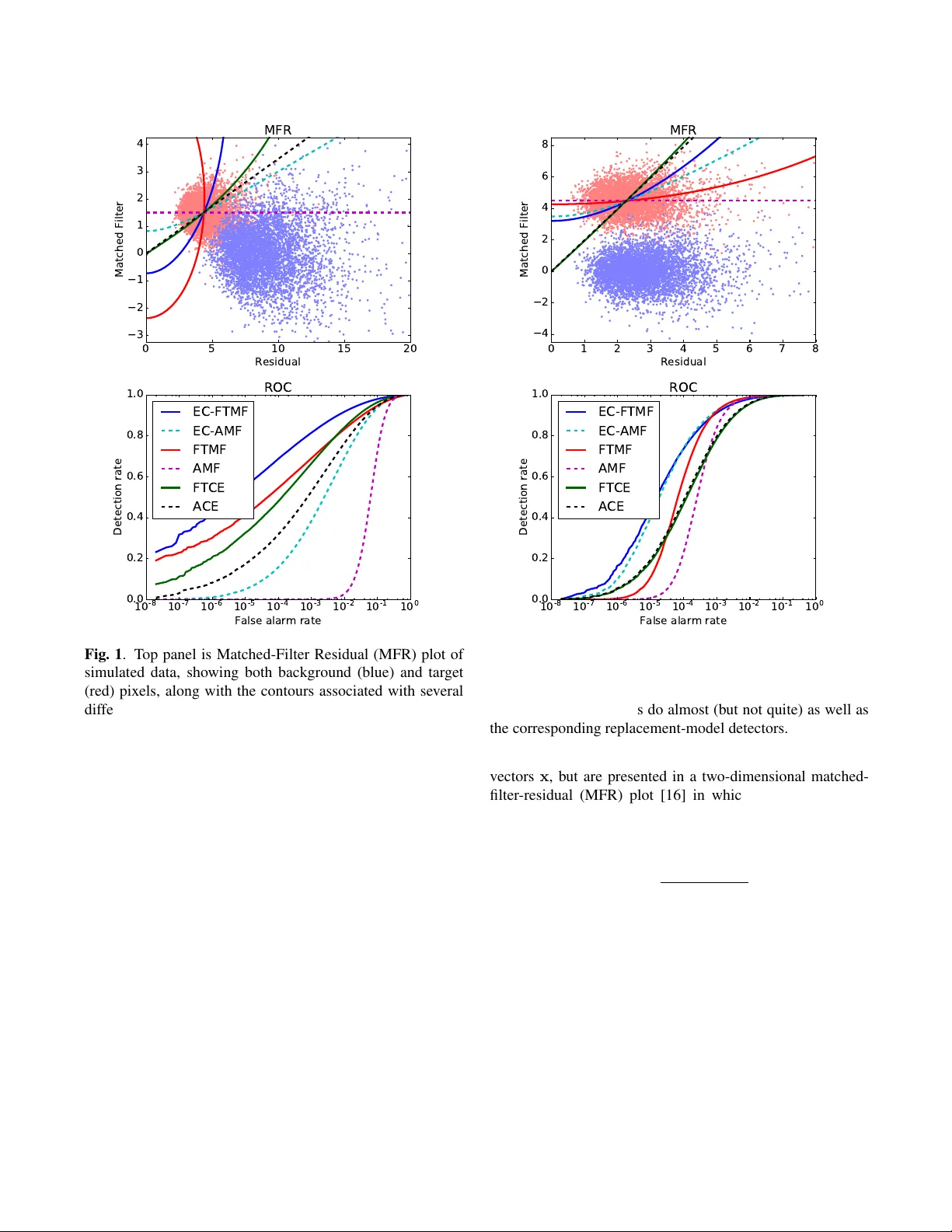
CLOSED-FORM DETECTOR FOR SOLID SUB-PIXEL T ARGETS IN MUL TIV ARIA TE T -DISTRIBUTED B A CKGR OUND CLUTTER J ames Theiler a , Beate Zimmer b , and Amanda Ziemann a a Space Data Science and Systems Group, Los Alamos National Laboratory , Los Alamos, NM b Department of Mathematics and Statistics, T exas A&M Uni versity–Corpus Christi, Corpus Christi, TX ABSTRA CT The generalized likelihood ratio test (GLR T) is used to deriv e a detector for solid sub-pixel targets in hyperspectral imagery . A closed-form solution is obtained that optimizes the replacement target model when the background is a fat- tailed elliptically-contoured multiv ariate t -distrib ution. This generalizes GLR T -based detectors that have pre viously been deriv ed for the replacement tar get model with Gaussian back- ground, and for the additiv e target model with an elliptically- contoured background. Experiments with simulated hyper- spectral data illustrate the performance of this detector in various parameter re gimes. Index T erms — Adaptive signal detection, algorithms, data models, detectors, multidimensional signal processing, pattern recognition, remote sensing, spectral image analysis. 1. INTR ODUCTION T o detect small targets in cluttered backgrounds requires models of the target, of the background, and of ho w the two interact. Although target variability models are important, particularly for solid tar gets [1], we will tak e the tar get signature as a single vector . Ho wever , we will consider a range of elliptically-contoured background models, from Gaussian to very fat tailed, and we will consider tw o dif ferent target-background interaction models – the additi ve model and the replacement model – that incorporate v ariability into the str ength of the target. 1.1. Background models The importance of background modeling has recently been emphasized [2], and although the Gaussian model is often surprisingly ef fective, a useful extension is the multi variate t - distribution, which has in particular been proposed for hyper - spectral imagery [3]. This is similar to the Gaussian in that it is defined by a mean and a covariance matrix, which implies that the distrib ution is uni-modal with ellipsoidal contours of This work was supported in part by the United States Department of Energy N A-22 project on Hyperspectral Advanced Research and Dev elop- ment for Solid Materials (HARD Solids). constant density; this density decreases with distance from the mean, but the decrease can be much slo wer than the exp( − r 2 ) decay e xhibited by Gaussians, leading to heavier tails that are often more representativ e of observed data. 1.2. T arget-backgr ound interaction models In many signal detection applications, the signal of interest is assumed to be additive with respect to a background that is generally characterized in some statistical way . W e can write x = z + α t (1) where x ∈ R d is the measured signal, z ∈ R d is the back- ground signal, t ∈ R d is the signal of interest, d is the number of spectral channels, and α is a scalar quantity that character - izes the strength of the signal. The additi ve model is the basis for many traditional target detection algorithms, including the adaptiv e matched filter (AMF) [4] and the adaptiv e coherence estimator (A CE) [5]. When the background is multiv ariate t , then the GLR T solution for the additiv e model leads to a detector we will here call the elliptically-contoured adapti ve matched filter 1 (EC-AMF) [6]; it is giv en by D ( x ) = p ( ν − 1) t T R − 1 ( x − µ ) q ( ν − 2) + ( x − µ ) T R − 1 ( x − µ ) , (2) where µ is the mean and R is the cov ariance matrix of the background distribution. In Eq. (2), ν → ∞ leads to the AMF detector , and ν → 2 leads to the A CE detector . While the additiv e model is the basis for many target detection algorithms, it has limitations [7], and in particular does not account for the occlusion of the background by a solid target. In the replacement model [8, 9], we treat 0 ≤ α ≤ 1 as the tar get area (fraction of a pixel), and write x = (1 − α ) z + α t . (3) This is called the replacement model because a fraction α of the background signal z is replaced with tar get signal t . The 1 In [6], it is giv en a dif ferent name (EC-GLR T) that is not as consistent with the naming con ventions used in this paper . finite target matched filter (FTMF), deri ved by Schaum and Stocker [10], is the replacement-model version of the AMF: it is the GLR T solution to Eq. (3) in the situation that the background z is Gaussian. Although this detector is some- what more complicated than the AMF , or ev en the EC-AMF in Eq. (2), it can be written as a closed-form expression. Closed-form generalizations of the FTMF hav e been deriv ed for Gaussian tar get v ariability [11] and alternativ e models of cov ariance scaling [12]. Here, we derive a closed- form GLR T solution when the background is a general class of elliptically-contoured distribution. In the special case that the background is Gaussian, we obtain the FTMF solution. W e treat the target detection problem in a hypothesis testing framework, with the null hypothesis corresponding to α = 0 and the alternati ve associated with α > 0 . Since the nonzero α is unspecified, this is a composite hypothesis testing problem [13], and we use the generalized likelihood ratio test (GLR T) to derive our detector . The detector is a function of x gi ven by the logarithm of this ratio D ( x ) = log max α p x ( x | α ) p x ( x | 0) . (4) The expression in Eq. (4) is written in terms of p x , which is the probability density function for x . W e can express this function in terms of p z ( z ) , the probability density associated with the background z . W e hav e p x ( x | α ) = (1 − α ) − d p z (( x − α t ) / (1 − α )) (5) where the ar gument ( x − α t ) / (1 − α ) is obtained by solving Eq. (3) for z , and where the prefactor (1 − α ) − d arises from the Jacobian of the transformation of variables from p x to p z . T aking z to have mean µ and cov ariance R , the multi- variate t distribution is gi ven by p z ( z ) = c | R | − d/ 2 1 + ( z − µ ) T R − 1 ( z − µ ) ν − 2 ! − d + ν 2 (6) where d is number of spectral channels, ν is a parameter that specifies how f at-tailed the distribution is (lar ger ν is less fat- tailed, with the ν → ∞ limit corresponding to a Gaussian distribution), and the normalizing constant c depends only on d and ν . Thus, p x ( x | α ) =(1 − α ) − d p z (( x − α t ) / (1 − α )) (7) = c | R | − d/ 2 (1 − α ) d 1 + w T R − 1 w (1 − α ) 2 ( ν − 2) ! − d + ν 2 (8) where w = ( x − µ ) − α ( t − µ ) . T o find the value of α that maximizes Eq. (8), we can take the deriv ative of log p ( x | α ) with respect to α , set that e xpression to zero, and solve for α . For Gaussian p z ( z ) , that approach was found [10] to produce a quadratic equation in α . For the more general multiv ariate t - distribution, we also obtain a quadratic equation, though with T able 1 . T axonomy of detection algorithms. The EC-FTMF (and its special case FTCE) are introduced in this paper , to extend the FTMF algorithm to non-Gaussian backgrounds. Gaussian Multiv ariate t Fat-tailed T arget model ν → ∞ 2 ≤ ν ≤ ∞ ν → 2 Additiv e AMF [4] EC-AMF [6] A CE [5] Replacement FTMF [10] EC-FTMF FTCE modified coefficients. The solution to that quadratic equation is giv en by b α = 1 − − B + p B 2 − 4 AC 2 A (9) where A = ( t − µ ) T R − 1 ( t − µ ) + ( ν − 2) , (10) B = (1 − ν /d )( x − t ) T R − 1 ( t − µ ) , (11) C = − ( ν /d )( x − t ) T R − 1 ( x − t ) . (12) This v alue of α satisfies p x ( x | b α ) = max α p x ( x | α ) . Thus, our detector , the elliptically-contoured finite target matched filter (EC-FTMF), is giv en by D ( x ) = log p x ( x | b α ) − log p x ( x | 0) (13) with p x ( x | α ) gi ven in Eq. (8) and b α given by Eqs. (9-12). In the ν → ∞ limit, the multi v ariate t becomes Gaussian, and the expressions in Eqs. (10-12) div erge. But in Eq. (9) it is only the relativ e values that matter; thus we can express this limit with the expressions B / A = − ( x − t ) T R − 1 ( t − µ ) /d, (14) C / A = − ( x − t ) T R − 1 ( x − t ) /d. (15) These values recapitulate the FTMF result obtained for a Gaussian background [10]. For ν → 2 , we hav e the heavy-tailed limit A = ( t − µ ) T R − 1 ( t − µ ) , (16) B = (1 − 2 /d )( x − t ) T R − 1 ( t − µ ) , (17) C = − (2 /d )( x − t ) T R − 1 ( x − t ) , (18) which we call the finite target coherence estimator (FTCE). W e remark that these three replacement-model detectors, the general EC-FTMF and the special cases FTMF and FTCE, hav e corresponding detectors associated with the additive model in Eq. (1), as shown in T able 1. These additive-model detectors are the EC-AMF and its special cases, AMF and A CE. For very small α and very large target magnitude | t | , we expect these replacement-model detectors to be well approximated by their associated additive-model detectors. In this sense, we can ar gue that the EC-FTMF detector described in Eq. (13) cov ers all six cases. 0 5 1 0 1 5 2 0 R e si d u a l − 3 − 2 − 1 0 1 2 3 4 M a t c h e d F i l t e r M F R 1 0 - 8 1 0 - 7 1 0 - 6 1 0 - 5 1 0 - 4 1 0 - 3 1 0 - 2 1 0 - 1 1 0 0 F a l se a l a r m r a t e 0 . 0 0 . 2 0 . 4 0 . 6 0 . 8 1 . 0 D e t e c t i o n r a t e R O C E C - F T M F E C - A M F F T M F A M F F T C E A C E Fig. 1 . T op panel is Matched-Filter Residual (MFR) plot of simulated data, showing both background (blue) and target (red) pixels, along with the contours associated with se veral different detection algorithms. The contours are chosen so that the detection rate is e xactly 0.5; the better detectors are those with fewer f alse alarms, which are associated with blue pixels that are “abo ve” the contours. Bottom panel is Receiver Operating Characteristic (R OC) curves for these detectors. Here, ν = 10 , d = 90 , T = 3 , and α = 0 . 5 . 2. SIMULA TION W e can illustrate the performance of the EC-FTMF detector on simulated data. In this simulation we draw N samples from a d -dimensional multiv ariate t -distrib ution parameter- ized by ν , with (for simplicity) zero mean and unit covari- ance. These N samples are representati ve of background pix- els from a multi- or hyper-spectral image that hav e been de- meaned and whitened. For each background sample, we used the matched-pair formulation [14, 15] to produce an associated target pixel, produced by the replacement model in Eq. (3) using a fixed value of α (which we know , but the algorithm does not). Our target signature t is given by a v ector of magnitude T . The background and target pixels are d -dimensional 0 1 2 3 4 5 6 7 8 R e si d u a l − 4 − 2 0 2 4 6 8 M a t c h e d F i l t e r M F R 1 0 - 8 1 0 - 7 1 0 - 6 1 0 - 5 1 0 - 4 1 0 - 3 1 0 - 2 1 0 - 1 1 0 0 F a l se a l a r m r a t e 0 . 0 0 . 2 0 . 4 0 . 6 0 . 8 1 . 0 D e t e c t i o n r a t e R O C E C - F T M F E C - A M F F T M F A M F F T C E A C E Fig. 2 . Here, ν = 10 , d = 10 , T = 30 , and α = 0 . 15 . The target is strong ( T  1 ) and small ( α  1 ), so the effect due to occlusion is limited, but still discernible. Here, the additiv e-model detectors do almost (but not quite) as well as the corresponding replacement-model detectors. vectors x , but are presented in a two-dimensional matched- filter-residual (MFR) plot [16] in which the matched-filter magnitude MF is plotted on the y -axis and the residual R is on the x -axis. In this zero-mean unit-cov ariance case: MF = t T x /T (19) R = q x T x − ( MF ) 2 . (20) Fig. 1 illustrates these pixels as points in a scatter -plot. The reason for choosing this representation is that all of the detectors we consider here have contours that can be plot- ted in this two-dimensional space. Fig. 1 also compares the performance of v arious detectors on this simulated data, and for these parameters, we see that the new EC-FTMF detec- tor does well. The original FTMF is confounded because it incorrectly assumes the background is Gaussian; the A CE, AMF , and EC-AMF detectors are confounded because they incorrectly assume the additiv e target model. In the regime of very large T and very small α , the replacement model is “nearly” additiv e. In Fig. 2, we observe that the replacement-model and additi ve-model variants of the same detectors are similar, although EC-FTMF is still discernibly better than EC-AMF , and FTMF is substantially better than AMF . Interestingly , FTCE is no better than A CE. W e have observ ed (results not shown here) that larger T and smaller α lead to a regime in which replacement-model and additiv e-model variants are virtually identical. 3. DISCUSSION In introducing the EC-FTMF detector , and sho wing that the GLR T solution can be expressed in closed form, we obtain a target detection algorithm that is both con venient and adapt- iv e to a range of conditions. In practice, using EC-FTMF (just as in using EC-AMF or other EC-based algorithms), one must estimate the multiv ariate t -distribution parameter ν that describes the fatness of the tails. T o keep things simple, our simulations employed the same ν in the algorithm that was used for the simulation. But estimation of the single scalar pa- rameter ν from a large dataset is not that dif ficult; one simple approach employs higher moments of the whitened data [17]. Finally , we remark that the GLR T – although widely used, and very often with good results – is not the only or necessarily the optimal solution to the composite hypothesis testing problem. One may prefer Bayesian approaches [13] or the recently introduced clairvo yant fusion [18, 19]. 4. REFERENCES [1] T . L. Myers, C. S. Brauer , Y .-F . Su, T . A. Blake, R. G. T onkyn, A. B. Ertel, T . J. Johnson, and R. L. Richardson, “Quantitativ e reflectance spectra of solid powders as a function of particle size, ” Applied Optics , v ol. 54, pp. 4863–4875, 2015. [2] S. Matteoli, M. Diani, and J. Theiler , “ An overvie w background modeling for detection of targets and anomalies in hyperspectral remotely sensed imagery , ” IEEE J. Sel. T opics in Applied Earth Observations and Remote Sensing , v ol. 7, pp. 2317–2336, 2014. [3] D. Manolakis, D. Marden, J. K erekes, and G. Shaw , “On the statistics of hyperspectral imaging data, ” Pr oc. SPIE , vol. 4381, pp. 308–316, 2001. [4] I. S. Reed, J. D. Mallett, and L. E. Brennan, “Rapid con vergence rate in adaptiv e arrays, ” IEEE T rans. Aer ospace and Electr onic Systems , vol. 10, pp. 853– 863, 1974. [5] S. Kraut, L. L. Scharf, and R. W . Butler , “The Adapt- iv e Coherence Estimator: a uniformly most-powerful- in variant adaptive detection statistic, ” IEEE T rans. Signal Pr ocessing , vol. 53, pp. 427–438, 2005. [6] J. Theiler and B. R. Foy , “EC-GLR T: Detecting weak plumes in non-Gaussian hyperspectral clutter using an elliptically-contoured generalized likelihood ratio test, ” Pr oc. IEEE International Geoscience and Remote Sens- ing Symposium (IGARSS) , p. I:221, 2008. [7] A. Schaum, “Enough with the additi ve target model, ” Pr oc. SPIE , v ol. 9088, p. 90880C, 2014. [8] A. D. Stocker and A. P . Schaum, “ Application of stochastic mixing models to h yperspectral detection problems, ” Pr oc. SPIE , vol. 3071, pp. 47–60, 1997. [9] D. Manolakis, C. Siracusa, and G. Shaw , “Hyperspectral subpixel target detection using the linear mixing model, ” T rans. Geoscience and Remote Sensing , vol. 39, pp. 1392–1409, 2001. [10] A. Schaum and A. Stock er, “Spectrally selecti ve tar - get detection, ” Pr oc. ISSSR (International Symposium on Spectr al Sensing Resear ch) , p. 23, 1997. [11] R. S. DiPietro, D. G. Manolakis, R. B. Lockwood, T . Cooley , and J. Jacobson, “Performance e valuation of hyperspectral detection algorithms for sub-pixel ob- jects, ” Pr oc. SPIE , vol. 7695, p. 76951W , 2010. [12] A. Schaum, “Continuum fusion solutions for replace- ment target models in electro-optic detection, ” Applied Optics , vol. 53, pp. C25–C31, 2014. [13] E. L. Lehmann and J. P . Romano, T esting Statistical Hypotheses . New Y ork: Springer , 2005. [14] J. Theiler , “Matched-pair machine learning, ” T ec hno- metrics , vol. 55, pp. 536–547, 2013. [15] ——, “T ransductive and matched-pair machine learning for difficult tar get detection problems, ” Proc. SPIE , vol. 9088, p. 90880E, 2014. [16] B. R. Foy , J. Theiler, and A. M. Fraser , “Decision boundaries in two dimensions for target detection in hyperspectral imagery , ” Optics Express , vol. 17, pp. 17 391–17 411, 2009. [17] J. Theiler , C. Scov el, B. W ohlber g, and B. R. Foy , “Elliptically-contoured distributions for anomalous change detection in hyperspectral imagery , ” IEEE Geo- science and Remote Sensing Lett. , vol. 7, pp. 271–275, 2010, the moment method for estimating ν is described in the Appendix. [18] A. Schaum, “Continuum fusion: a theory of inference, with applications to hyperspectral detection, ” Optics Expr ess , vol. 18, pp. 8171–8181, 2010. [19] J. Theiler , “Confusion and clairvoyance: some remarks on the composite hypothesis testing problem, ” Pr oc. SPIE , vol. 8390, p. 839003, 2012.