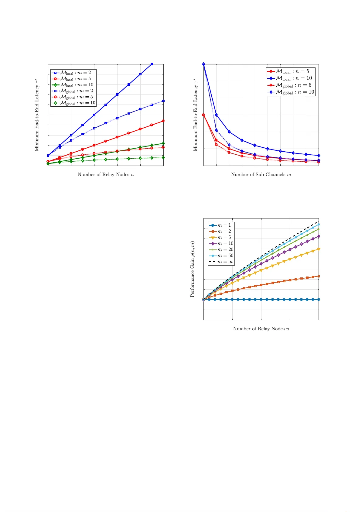
Traffic Allocation for Low-Latency Multi-Hop Networks with Buffers

1 T raf fic Allocation for Lo w-Latenc y Multi-Hop Networks with Buf fers Guang Y ang, Student Member , IEEE , Martin Haenggi, F ellow , IEEE , and Ming Xiao, Senior Member , IEEE Abstract —For buffer -aided tandem networks consisting of relay nodes and multiple channels per hop, we consider two traffic allocation schemes, namely local allocation and global allocation, and in vestigate the end-to-end latency of a file transfer . W e formulate the problem for generic multi-hop queuing systems and subsequently derive closed-form expressions of the end-to- end latency . W e quantify the advantages of the global allocation scheme relativ e to its local allocation counterpart, and we conduct an asymptotic analysis on the performance gain when the number of channels in each hop increases to infinity . The traffic allocations and the analytical delay performance are validated through simulations. Furthermor e, taking a specific two-hop network with millimeter -wav e (mm-wave) as an example, we derive lower bounds on the average end-to-end latency , where Nakagami- m fading is considered. Numerical results demonstrate that, compared to the local allocation scheme, the advantage of global allocation gr ows as the number of relay nodes increases, at the expense of higher complexity that linearly incr eases with the number of relay nodes. It is also demonstrated that a proper deployment of relay nodes in a linear mm-wave network plays an important role in reducing the average end-to-end latency , and the av erage latency decays as the mm-wave channels become more deterministic. These findings pr ovide insights for designing multi-hop mm-wave networks with low end-to-end latency . Index T erms —T raffic allocation, end-to-end latency , multi-hop networks, queuing, millimeter -wave communication. I . I N T RO D U C T I O N A. Backgr ound and Motivation In many future applications, lo w latency is a crucial quality-of-service (QoS) constraint [1]. For instance, vehicle- to-ev erything, remote surgery , and industrial control need the support of low-latency communications. Accordingly , the requirement on end-to-end latency in the fifth-generation (5G) mobile network and beyond, on the order of 1 to 5 ms, is much more stringent than that in 3G and 4G systems [2], [3]. Besides, to handle the unprecedented data volumes and hea vy traffic load in future wireless communications, large buf fers are usually used at transceiv ers. W ith these buffers, the data can be temporarily stored in a queue, until the corresponding service is av ailable for its deliv ery . The queuing delay is defined as the waiting time of a file in the buf fer or queue before being transmitted [4], [5]. For future wireless systems with buffers, the queuing delay becomes a key contributor This work was supported by EU Marie Curie Project, QUICK, No. 612652, and Wireless@KTH Seed Project “Millimeter W ave for Ultra-Reliable Low- Latency Communications”. G. Y ang and M. Xiao are with the Department of Information Science and Engineering (ISE), KTH Royal Institute of T echnology , Stockholm, Sweden (Email: {gy ,mingx}@kth.se). M. Haenggi is with the Department of Electrical Engineering, Uni versity of Notre Dame, Notre Dame, IN, 46556 USA. (E-mail:mhaenggi@nd.edu) to the ov erall latency , since the heavy network traffic may produce significant data backlog in buffers. Thus, one of the most effecti ve ways for achie ving lower latency is to reduce the queuing delay . It is worth mentioning that, as one k ey enabler of high data- rate transmissions, millimeter-wa ve (mm-wave) technologies hav e raised extensi ve research interest and hav e been regarded as promising candidates in future mobile networks [6 ]–[8]. Motiv ated by the huge potential of using mm-wa ve in v arious scenarios, in this work, we restrict ourselves to mm-wav e bands to in vestigate the traffic allocations over multi-hop networks. In this work, we consider a linear multi-hop network that consists of a source node, a destination node, and multiple buf fer-aided relay nodes, where parallel channels in each hop are also assumed. This network architecture is promising for future mobile networks and motiv ated by the following two facts: (i) Unlike wireless communications in sub- 6 GHz bands, mm-wa ve radios used in future mobile systems encounter much more sev ere path loss, which may restrict the range of wireless communications. One solution to enlarge the range of mm-wav e communications is to use relay nodes. W ith the multi-hop architecture, the distance between ad- jacent nodes is shortened, thereby mitigating the serious path loss in mm-wav e bands. (ii) The consideration of se veral parallel channels in each hop mainly stems from the application of distributed antenna systems (DAS) or remote radio heads (RRH). Note that sharp beams are generated by the dense antenna elements in mm-wave bands. With D AS or RRH, multiple channels can be established between communication nodes with negligible inter-channel interference. Multiple channels in good conditions can be selected via proper channel esti- mation and tracking techniques, thereby enabling higher performance for mm-wave communications. It is important to in vestigate the end-to-end latency for networks with the aforementioned multi-hop multi-channel architecture. Howe ver , this system model is rarely studied, especially when buffers are incorporated at relay nodes. B. Related W orks In the past few years, numerous efforts hav e been dev oted to the research on latency in multi-hop networks with buf fers, and remarkable progress has been reported. In [9], the a verage end-to-end delay in random access multi-hop wireless ad hoc networks was studied, and the analytical results were 2 discussed and compared with the well established information- theoretic results on scaling laws in ad hoc networks. For an opportunistic multi-hop cognitiv e radio network, the av erage end-to-end latency in the secondary network was studied in [10] by applying queuing theoretic techniques and a dif fusion approximation. In [11], the queuing delay and medium access distribution o ver multi-hop personal area networks was inv es- tigated. T o reduce the end-to-end latency in multi-hop queuing systems, many works have focused on various aspects such as the routing, scheduling, and traffic control. Using back- pressure methods, algorithms and analysis were widely in- vestigated in [12]–[15] for low-latency multi-hop wireless networks. For a two-hop half-duplex network with infinite buf fers at both the source and the relay node, the problem of minimizing the average sum queue length under a half- duplex constraint was in vestigated in [16]. Some efforts for systems with interference incorporated have also been made in the past decade. In [17], several QoS routing problems, i.e., end-to-end loss rate, end-to-end average delay , and end- to-end delay distribution, in multi-hop wireless network were considered, where an exact tandem queuing model was es- tablished, and a decomposition approach for QoS routing was presented. Using a tuple-based multidimensional conflict graph model, a cross-layer framew ork was established in [18], in order to inv estigate the distributed scheduling and delay-aware routing in multi-hop multi-radio multi-channel networks. Considering a multi-hop system that consists of one source, one destination, and multiple relays, the end-to-end delay performance under a TDMA-ALOHA medium access control protocol, with interferers forming a Poisson point process, was in vestigated in [19], and insights regarding delay- minimizing joint medium access control/routing algorithms were provided for networks with randomly located nodes. In the recent work [20], a distributed flow allocation scheme was proposed for random access wireless multi-hop networks with multiple disjoint paths, aiming to maximize the av erage aggregate flow throughput and guarantee a bounded packet delay . In spite of many significant achiev ements in multi-hop networks with b uffers, e.g., [11], [17], [21], [22], the research on traffic allocation to achiev e low-latency schemes is rather limited. In our recent work [23], two low-latenc y schemes for mm-wav e communications, namely traffic dispersion and network densification, were in vestigated in the framework of network calculus and effecti ve capacity . The analysis in [23] was performed for a giv en network setting, i.e., fixed trans- mission scheme, sum power budget, and arriv al rate for the whole network, and bounding techniques were used to explore the potential for lo w-latency communications. Ho we ver , traf fic allocations for reducing the latenc y were not in vestigated, and the potential performance gain by optimized traffic allocations was not quantified. C. Objective and Contributions For multi-hop networks with multiple channels in each hop, an optimized traffic allocation scheme plays a crucial role when incorporating queues [24], since the traffic congestion at the relay nodes due to non-optimized allocation may produce long queues, resulting in larger end-to-end latency [5]. Con- ventionally , the method for studying low-latenc y networks is to transfer the objecti ves into network optimization problems, i.e., problems in [25]. Howe ver , these graph-based approaches do not apply to the scenarios with buf fers. Therefore, it is necessary to in vestigate the latency optimization problem for buf fered networks in a different way . The main objectiv e of our work is to dev elop an efficient traffic allocation scheme for mm-wa ve networks that minimize the end-to-end latency 1 . Specifically , we consider a linear multi-hop buffer -aided networks with multiple channels in each hop. The main contributions of our work are summarized as follo ws: • Focusing on two traf fic allocation schemes, namely , local allocation and global allocation, we calculate the end-to- end latency for deliv ering a fixed-length message from the source to the destination. Furthermore, we analyti- cally compare these two allocation schemes through the relativ e performance gain and in vestigate the benefits of global allocation. • For multi-hop buffered networks with multiple channels in each hop, we e xploit the recursiv e nature of the global allocation scheme. Thus, there is no need to search for the optimal solution in an exhaustiv e manner . The recursive method introduced in this paper significantly simplifies the global minimization of the end-to-end latency and provides insights for analyzing tandem queuing systems. Besides, we give the ov erall computational complexity for performing local or global allocations. • Follo wing the recursive characterization for global alloca- tion, we present the asymptotic relati ve performance gain when the number of per-hop channels goes to infinity . Furthermore, based on traf fic allocation schemes that can be applied to generic multi-hop networks, we specifically consider a two-hop linear mm-wa ve network and in ves- tigate the average end-to-end latency , with Nakagami- m fading incorporated. W e derive lower bounds of the av erage end-to-end latency for two allocation schemes. I I . S Y S T E M M O D E L A N D P R O B L E M F O R M U L AT I O N A. System Model W e consider a multi-hop system, which consists of multiple buf fer-aided relay nodes and multiple channels in each hop. The first-in-first-out (FIFO) rule applies to the queues at the buf fer-aided relay nodes. As illustrated in Fig. 1, given n tandem relay nodes, we label all nodes in reverse order , i.e., from the destination to the source, to simplify the notation in the following analysis. That is, the destination and the source are labeled as node 0 and node n + 1 , respectiv ely . The hop between node h and node h + 1 is denoted by hop h , for all h ∈ { 0 } ∪ [ n ] . In addition, we assume there are m h channels in hop h , and we denote by C h , k the capacity of the k th channel 1 The traffic allocations discussed in this paper can be generalized to networks at other frequency bands, e.g., those used in 3G/4G systems, while mm-wav e is just taken as an important e xample for study here. 3 in hop h for all k ∈ [ m h ] . W e define [ N ] , { 1 , 2 , . . . , N } for any N ∈ N . Regarding the channels in each hop, as aforementioned, due to the negligible multi-path effect and the high directivity of mm-wa ve beams, the small-scale fading is very weak. W e denote by C h , k the channel capacity . First we assume no fading for the inv estigation in Sec. III and Sec. IV, thereby producing results for general networks with fixed capacities ov er all channels. In the following Sec. V, Nakagami- m fading is added to the model. This modeling preserves the actual main characteristics of mm-wav e channels in practice, and also provides high tractability for the following analysis. In this work, we assume that the traffic allocation that assigns the traffic to the individual channels is performed at the source and relay nodes. That is, the traf fic arri ving at one node is decomposed into sev eral fractions according to the giv en allocation scheme, and those fractions are subsequently pushed onto the channels and deliv ered to the next node, where each fraction is partitioned again. For the traf fic allocation with respect to channels in hop h , we define the vector α h ,  α h , 1 , α h , 2 , . . . , α h , m h  ∈ R m h + for all h ∈ { 0 } ∪ [ n ] , which is subject to the follo wing constraint ∥ α h ∥ 1 , m h  i = 1 α h , i = 1 , (1) where ∥ · ∥ 1 represents the 1 -norm for vectors. The traffic allocation α h is determined by the capacities of outgoing channels, such that the incoming fraction can be accordingly chopped down and reallocated onto the respectiv e outgoing channels. It is worth noting that the traffic allocation α h is performed at node h + 1 . W e assume multiple parallel servers at the source node and the relay nodes (the number of servers equals the number of outgoing channels), such that fractions can be transmitted ov er the different channels at the same time. This model follows a special variant of general fork-join systems [ 26], [27] (with a synchronization constraint), where all tasks of a job start ex ecution simultaneously , and the job is completed when the final task leav es the system. Relay nodes are full- duplex but only equipped with a single buf fer such that the data reception and transmission can be performed at the same time and the receiv ed fractions leav e the buf fer one by one. At each relay node, one fraction is not served (chopped into smaller fractions and forwarded to the next node) until it is completely receiv ed. In future mobile networks, the capacity of mm-wav e channels can reach multi-gigabits per second and the packet size is around se veral kilobits or megabits at most [28], and hence the latency is of the order of milliseconds or ev en smaller . In this sense, compared to the scheme that allows to receiv e and transmit a fraction simultaneously , the setting that a fraction has to be recei ved entirely before it can be forwarded o ver the next hop definitely produces higher latenc y (but not significantly), while a voiding the potential interference induced by simultaneous transmission and reception. Further- more, we assume that the file is infinitely divisible, i.e., any fraction can be divided into smaller pieces with arbitrarily small size. Aiming to inv estigate the limits of low latency , we assume infinite divisibility throughout our work for theoretical purposes. Howe ver , for communication systems in practice, there always exists an atomic unit for constituting files, such that a file cannot be infinitely divisible. Hence, the delay performance obtained in this work is de graded if the practical constraint of finite divisibility is incorporated. It is worth mentioning that the assumption of infinite di visibility does not imply a fluid-flow model (although it is one of the typical features), since there are two phases, i.e., fraction reception and fraction transmission, at any intermediate node, rather than following the continuous manner in fluid-flow models. B. Pr oblem F ormulation For the transmission from the source to the destination, we consider two traffic allocation schemes, namely , local traffic allocation and global traffic allocation. T o simplify the exposition, M local and M global are used to denote the local and global allocation scheme, respecti vely , which are described as follows. • M local : Node h for all h ∈ [ n + 1 ] only has the capacity information of the channels in hop h − 1 . The traffic allocation performed at node h only optimizes the trans- mission ov er channels in hop h − 1 . This scheme ensures that the latency in the local hop is minimized, but is oblivious to the traf fic allocations in other hops. • M global : Node h for all h ∈ [ n + 1 ] has the entire capacity information of all channels from hop 0 to hop h − 1 . The traffic allocation performed at node h not only relies on channels in hop h − 1 , but also relies on channels in the remaining hops, i.e., from hop 0 to hop h − 1 . This scheme minimizes the latency through h hops The definition of the end-to-end latency in our study is gi ven as follo ws: Definition 1 (End-to-End Latency) . Given traffic allocations { α h } , h ∈ { 0 } ∪ [ n ] , for all hops, the end-to-end latency τ n  α n , α n − 1 , . . . , α 0  (also written as τ n in the sequel for notional simplicity) of the tandem queuing system with n r elay nodes is defined as the time to deliver one fixed-length file of size 1 (without loss of generality) from the sour ce to the destination 2 , describing the time span fr om the moment the sour ce starts transmission to the moment all fractions ar e r eceived at the destination. The definition above indicates that the latency takes into account both the time of traversing the wireless channels (service time) and the time of queuing in buf fers (waiting time) at the relays. For exposition, we consider a simple network as an example to illustrate the end-to-end latency and the difference between M local and M global , where n = 1 , m 1 = 2 , and m 0 = 1 . In this specific network, traf fic allocation α 1 ,  α 1 , 1 , α 1 , 2  is performed over hop 1 , while there is no traf fic allocation over hop 0 , i.e., α 0 = 1 . The service time for fraction α i , j ov er the channel with capacity C i , j is characterized by their quotient, i.e., α i , j C − 1 i , j . It is worth noting 2 For generality and notational simplicity , we do not assign units to the file size and channel capacities, i.e., they are all normalized. For a concrete network, the most suitable units can be chosen, e.g., the file size (and, in turn, the fractions) could be measured in MB, and the capacities in Mb/s. 4 Fig. 1. Illustration of a multi-hop system, consisting of multiple relay nodes are multiple channels in each hop. that, due to the adoption of buf fer at node 1, the arri val order of dif ferent fractions should also be taken into account. Hence, in addition to the service time, the potential waiting time for the latter incoming fraction also contributes to the end-to-end latency τ 2 . Then τ 2 is obtained as τ 2  α 1 , α 0  =                    max        C − 1 0 , 1 + α 1 , 1 C − 1 1 , 1 , α 1 , 2  C − 1 0 , 1 + C − 1 1 , 2         , α 1 , 1 C 1 , 1 ≤ α 1 , 2 C 1 , 2 max        C − 1 0 , 1 + α 1 , 2 C − 1 1 , 2 , α 1 , 1  C − 1 0 , 1 + C − 1 1 , 1         , otherwise . (2) From (2), we see that the end-to-end latency considered in this work is dif ferent from those that consider either the service time or the waiting time only . Thus, the conv entional techniques for graph-based network optimization or queuing systems are not applicable. Since the traffic allocation only occurs at hop 1 , the resulting minimization problem regarding τ 2 can be formulated as τ ∗ 2 = min ∥ α 1 ∥ = 1 τ 2  α 1 , α 0  = τ 2  α ∗ 1 , α 0  , (3) where α ∗ 1 representing the optimum traffic allocation differs for M local and M global . F ollowing the distinct mechanisms of M local and M global , we have: • for M local , since the channel information at the local hop is adopted for optimization, α ∗ 1 is obtained as α ∗ 1 = arg min ∥ α 1 ∥ = 1 max  α 1 , 1 C − 1 1 , 1 , α 1 , 2 C − 1 1 , 2  . (4) • for M global , since the channel information over all hops is adopted for optimization, α ∗ 1 is obtained as α ∗ 1 =                    arg min ∥ α 1 ∥ = 1 max        C − 1 0 , 1 + α 1 , 1 C − 1 1 , 1 , α 1 , 2  C − 1 0 , 1 + C − 1 1 , 2         , α 1 , 1 C 1 , 1 ≤ α 1 , 2 C 1 , 2 arg min ∥ α 1 ∥ = 1 max        C − 1 0 , 1 + α 1 , 2 C − 1 1 , 2 , α 1 , 1  C − 1 0 , 1 + C − 1 1 , 1         , otherwise . (5) Evidently , M global targets to the objectiv e function τ 2 straight- forwardly for optimization, while M local can only gi ve a sub- optimal solution via meeting the local optimization constraint. It is worth noting that, when more hops and/or parallel channels on each hop are incorporated, it is not possible to provide a closed-form expression for the end-to-end latency (as giv en in (2)), since the orders of arri val of the fractions at different nodes become rather complicated. I I I . T R A FFI C A L L O C A T I O N F O R M U LT I - H O P N E T W O R K S In this section, we will in vestigate the optimized end-to- end latency . In the analysis, the exact traffic allocations at the source and all relay nodes are presented, and the over - all computational complexity for different traffic allocation schemes are briefly discussed subsequently . For generality , the capacities of parallel channels on each hop are distinguished by distinct notations. For specific scenarios considering the sum-capacity constraint, the bandwidth can be partitioned in any manner to implement parallel channels with arbitrarily distributed capacities. W e use “big- O ” notation to characterize the ov erall compu- tational complexity for M local and M global . The definition of the “big- O ” notation is giv en as follows: assuming u ( x ) and f ( x ) are functions defined on some subset X ⊂ R , O ( f ( x )) denotes the set of all functions u ( x ) such that | u ( x )/ f ( x ) | stays bounded, i.e., O ( f ( x )) ,  u ( x ) : sup x ∈ X | u ( x )/ f ( x ) | < ∞  . (6) Clearly , we have O ( f 1 ( x ) ) ⊂ O ( f 2 ( x ) ) if we have | f 1 ( x ) | ≤ | f 2 ( x ) | ov er all x ∈ X . A. Latency for Networks Using M local Before deriving the minimum latency with M local , we start from a single-hop system, as shown in Fig. 2. T o simplify the notation, we assume that there are m channels between the source and the destination, where C i for i ∈ [ m ] de- notes the capacity of the i th channel. The traffic allocation α , [ α 1 , α 2 , . . . , α m ] is performed at the source node. In the follo wing Lemma 1, the optimal traf fic allocation at the source node is presented, and the resulting minimum end- to-end latency for the system sho wn in Fig. 2 is also deri ved. Lemma 1. Given m channels with capacity C i for i ∈ [ m ] between the source and the destination, letting α i ∈ ( 0 , 1 ) 5 Fig. 2. Illustration of a single-hop system with multiple channels between the source and the destination. denote the fraction of the traf fic allocated to the i th channel with capacity C i , the minimum end-to-end latency is τ ∗ =  m  i = 1 C i  − 1 , (7) achie ved by α i = C i   m j = 1 C j  − 1 for all i ∈ [ m ] . Pr oof. According to the mechanism of M local , we know that the minimum latency comes from applying the optimal traffic allocation α ∗ , i.e., α ∗ = arg min ∥ α ∥ = 1 max 1 ≤ i ≤ m  α i C − 1 i  , (8) which is solved as α i = C i   m j = 1 C j  − 1 for all i ∈ [ m ] . Then the minimum end-to-end latency τ ∗ can be obtained by applying α ∗ .  From Lemma 1, we notice that M local = M global optimizes the traffic allocations such that all fractions arrive at the destination at the same time. Besides, from the perspectiv e of the end-to-end delay , it is equi v alent to having a single channel with the sum capacity when applying M local for multiple channels. Based on Lemma 1, the optimal local traffic allocation and the resulting minimum latency for the multi-hop system in Fig. 1 are obtained in Theorem 1. Theorem 1. F or the tandem network in F ig. 1 with n relay nodes and m h channels in the h th hop, the minimum end-to-end latency with M local is τ ∗ n = n  h = 0  m h  k = 1 C h , k  − 1 , (9) achie ved by α h , k = C h , k   m h j = 1 C h , j  − 1 . Pr oof. W ith M local , the objective is to ensure that all fractions can reach the next adjacent node simultaneously . According to Lemma 1, in hop h the minimum latency is w ∗ h ,   m h k = 1 C h , k  − 1 . Note that the traffic allocation is performed independently and sequentially from hop n to hop 0 . In this case, the minimum end-to-end latency can be obtained by summing up w ∗ h ov er all h ∈ { 0 } ∪ [ n ] , i.e., τ ∗ n ,  n h = 0 w ∗ h = Fig. 3. Illustration of a two-hop network, where multiple channels are between the source and the relay , and one channel between the relay to the destination.  n h = 0   m h k = 1 C h , k  − 1 , when the proper local allocation scheme is applied.  According to Theorem 1, it is not difficult to find that the end-to-end transmission with M local is equiv alent to trans- mitting the entire file hop by hop. Paired with Lemma 1, we know that all fractions are deli vered from one node to the next simultaneously , which is equiv alent to combining all sub-channels in each hop as a single channel with the sum capacity and moving the entire file through the network without partitioning. In this case, one relay node will buf fer the whole file, while the buffers at other relay nodes remain empty . In terms of efficienc y , the utilization of buf fers for the transmission is relati vely lo w , due to the une ven distrib ution of file fractions in the network. Furthermore, for networks with buf fers, it is worth noting that the end-to-end latency (see the example with respect to (2)) differs from the non-buf fered system, while the specific local scheme makes the resulting delay the same with the non-buf fered system since arri vals on each hop can reach the node at the same time when M local is applied. B. Latency for Networks Using M global Prior to inv estigating the optimized end-to-end latency with M global for the multi-hop network shown in Fig. 1, we consider a two-hop system sho wn in Fig. 3, where a buf fer-aided relay node is deployed between the source and the destination. W e assume m channels between the source and the relay node, and we denote by C i for i ∈ [ m ] the capacity of the i th channel. From the relay node to the destination, we assume that there is only one channel with capacity C 0 . The traffic allocation α , [ α 1 , . . . , α m ] is performed at the source node, while no allocation is performed at the relay node, due to the single channel between the relay node and the destination. In the follo wing Lemma 2, the optimal traf fic allocation at the source node and the resulting minimum end-to-end latency for the system shown in Fig. 3 are deri ved. Lemma 2. F or the two-hop system shown in F ig. 3, the minimum end-to-end latency is τ ∗ =  C − 1 m + C − 1 0  m − 1  k = 1 C k + 1  C − 1 k + C − 1 0  1 + m  i = 2 i − 1  k = 1 C k + 1  C − 1 k + C − 1 0  , (10) 6 achie ved by α i = i − 1  k = 1 C k + 1  C − 1 k + C − 1 0  1 + m  j = 2 j − 1  k = 1 C k + 1  C − 1 k + C − 1 0  . (11) Pr oof. Please see Appendix A.  Clearly , when applying the allocation in Lemma 2, one fraction reaches the relay node always at the time when the previous fraction has completely left the buf fer . In contrast to the scheme in Lemma 1, all fractions arrive at the relay node sequentially , rather than simultaneously . Thus, the length of the resulting queue is the length of file fraction, which is usually much smaller than that of the whole file. It is worth mentioning that the optimum traffic allocation giv en in Lemma 2 is not unique, i.e., there exist sev eral other solutions that achie ve the same minimum end-to-end latency . 1) M global for a two-hop network: Assuming the sum capacity for channels between the source and the relay is fixed, we ne xt inv estigate the impact of increasing the number of channels between the source and the relay on end-to-end latency for the two-hop network in Fig. 3. Giv en a fixed sum capacity , it is evident that τ ∗ depends on the individual capacities C i for i ∈ [ m ] . W e will study the best channel capacity allocation for minimizing τ ∗ in the following corollary . Note that the channel capacity allocation determines the channel capacities potentially via frequency division techniques, while the traffic allocation partitions the data traffic according to the given channel capacities. W e assume that the sum capacity for channels between the source and the relay is 1 without loss of generality . Corollary 1. F or the two-hop system in Fig . 3, given  m i = 1 C i = 1 with C i > 0 for i ∈ [ m ] , the channel allocation that minimizes τ ∗ is the uniform allocation, i.e., C i = m − 1 for all i ∈ [ m ] . Pr oof. Please see Appendix B.  Giv en a sum-capacity constraint, Corollary 1 indicates that the lo west end-to-end latency with M global can be achie ved via the uniform allocation, i.e., via splitting the bandwidth equally . Based on Corollary 1, the minimum end-to-end latency with C i = m − 1 for any i ∈ [ m ] is τ ∗ =  C 0  1 −  1 + ( mC 0 ) − 1  − m   − 1 , (12) achiev ed by α i =  1 + ( mC 0 ) − 1  i − 1 ( mC 0 ) − 1  1 + ( mC 0 ) − 1  m − 1 . (13) W e next in vestigate the monotonicity of τ ∗ in (12) and the asymptotic performance as m → ∞ . Corollary 2. F or the two-hop system in F ig. 3, assuming C i = m − 1 for all i ∈ [ m ] , τ ∗ monotonically decreases with m and τ ∗ →  C 0  1 − exp  − C − 1 0    − 1 , when m → ∞ , and the limiting traf fic allocation tends to be the uniform allocation. Pr oof. The monotonic decrease of τ ∗ with respect to m follo ws since  1 + x − 1  x increases with x . For the asymptotic latency , i.e., as m → ∞ , we hav e lim m →∞ τ ∗ = lim m →∞ C − 1 0  1 −  1 + ( mC 0 ) − 1  − m  − 1 = C − 1 0 lim m →∞  1 −   1 + ( mC 0 ) − 1  mC 0  − 1 C 0  − 1 = C − 1 0  1 −  lim m →∞  1 + ( mC 0 ) − 1  mC 0  − 1 C 0  − 1 =  C 0  1 − exp  − C − 1 0    − 1 . (14) W ith (13), we notice that lim m →∞ α i + 1 α i = lim m →∞  1 + ( mC 0 ) − 1  = 1 (15) for all i ∈ [ m ] , which indicates that the limiting traffic allocation reduces to the uniform allocation.  W ith a fixed sum capacity for channels between the source and the relay , it is demonstrated from Corollary 2 that it is always beneficial to increase the number of channels. This observation coincides with the well-known fact that di viding the bandwidth into as many fractions as possible is delay- optimum for full-duplex channels (see results, e.g., in [29]). Howe ver , this advantage diminishes as m grows, and the re- sulting end-to-end latency with M global approaches a constant limit, which only depends on C 0 . This corollary indicates that, with respect to a giv en sum capacity , it is better to have multiple channels with smaller capacity rather than one single channel with lar ger capacity , or to split the channel into sub- channels using frequenc y division. Also, it is worth noting that the asymptotic result is a lower bound on the latency for all cases where the sum capacity over the first hop is fixed, and the lo wer bound is determined by C 0 when applying M global . 2) Comparison with time division: In what follows, we consider a scenario that has only a single channel with capacity 1 (rather than multiple sub-channels shown in Fig. 2) in the source-relay hop (corresponding to the systems that have only a single server at the source node). The file is partitioned into fractions via the traffic allocation in the time domain, which are sequentially deliv ered from the source node. Follo wing the method for the proof of Lemma 2, the minimum latency can be achiev ed if the condition α i = C − 1 0 α i − 1 holds for all i ∈ [ m ] \ { 1 } . The performance for traffic allocation in the time domain with M global is gi ven as belo w . Lemma 3. Using time division, the minimum end-to-end latency τ ∗ with M local is τ ∗ = C − 1 0  m i = 0 C i 0  m − 1 i = 0 C i 0 = 1 − C m + 1 0 C 0 − C m + 1 0 , (16) achie ved by α i = C 1 − i 0 m − 1  k = 0 C − k 0 . (17) τ ∗ monotonically decreases with m , and τ ∗ → max  C − 1 0 , 1  when m → ∞ . 7 Pr oof. The detailed deriv ation for (16) is omitted since the method is similar to that in Appendix A. The monotonic decease of τ ∗ as m increases is evident by observing (16). For the limiting latency as m → ∞ , we have lim m →∞ τ ∗ = C − 1 0 lim m →∞  m i = 0 C i 0  m − 1 i = 0 C i 0 =  1 , C 0 ≥ 1 C − 1 0 , C 0 < 1 , (18) which can be summarized as lim m →∞ τ ∗ = max  C − 1 0 , 1  . There- fore, the proof is completed.  W e can see that the bottleneck channel (with smaller ca- pacity) in the tw o-hop system determines the limiting latency . Unlike Corollary 2, the file fractions are not simultaneously deliv ered from the source in Lemma 3. This traffic allocation is performed using time division techniques. It is worth mentioning that we aim to study the minimum latency among all feasible traffic allocations in the time domain. W e find that the optimal traffic allocation (with M global ) based on the time division follo ws a geometric progression with the scale factor C − 1 0 , while the uniform traffic allocation (with M local ), i.e., α i = m − 1 for i ∈ [ m ] , cannot achieve the optimum. For notational simplicity , we denote by τ ∗ f and τ ∗ t the minimum latency in (12) and (16), corresponding to the traffic allocations in the frequency domain and the time domain, respectiv ely . W e compare τ ∗ f and τ ∗ t for any positiv e integer m in the follo wing corollary . Corollary 3. τ ∗ f ≥ τ ∗ t holds for all m ∈ N . Pr oof. Note that for C 0 > 0 we hav e  C 0 + m − 1  m = m  i = 0 m − i  m i  C m − i 0 ≤ m  i = 0 C i 0 , (19) where the property  m i  ≤ m i for all i ∈ { 0 } ∪ [ m ] is applied, and the equality holds if m = 1 or i = 0 , 1 . Then we can obtain that  1 + ( mC 0 ) − 1  − m ≥ C m 0  m i = 0 C i 0 , (20) which leads to  1 −  1 + ( mC 0 ) − 1  − m  − 1 ≥  m i = 0 C i 0  m − 1 i = 0 C i 0 , (21) thereby concluding τ ∗ f ≥ τ ∗ t .  Corollary 3 demonstrates that, if the total channel capacity in the source-relay hop is fixed, the time-division traffic alloca- tion outperforms the frequency-di vision scheme in achieving the lo wer end-to-end latency . 3) M global for general network: Based on Lemma 2, for the multi-hop buf fer-aided network illustrated in Fig. 1, the optimal traf fic allocation at the source node and the resulting minimum end-to-end latency are giv en for M global in the following theorem. Theorem 2. F or the tandem network in F ig. 1 with n relay nodes and m h channels in the h th hop, the minimum end-to-end latency with M global is τ ∗ n =  C − 1 n , m n + τ ∗ n − 1  m n − 1  k = 1 C n , k + 1  C − 1 n , k + τ ∗ n − 1  1 + m n  i = 2 i − 1  k = 1 C n , k + 1  C − 1 n , k + τ ∗ n − 1  , (22) with initial condition τ ∗ 0 ,   m 0 i = 1 C 0 , i  − 1 , achie ved by α h , k =                          C h , k  m h  k = 1 C h , k  − 1 , h = 0 k − 1  i = 1 C h , i + 1  C − 1 h , i + τ ∗ h − 1  1 + m h  j = 2 j − 1  i = 1 C h , i + 1  C − 1 h , i + τ ∗ h − 1  , h ≥ 1 . (23) Pr oof. For h ∈ { 0 } ∪ [ n ] , we denote by τ ∗ h the minimum end- to-end latency from hop 0 to hop h . In addition, we define the effecti ve capacity as the reciprocal of minimum end-to-end latency , i.e., E h ,  τ ∗ h  − 1 . According to Lemma 1, the initial effecti ve capacity E 0 is gi ven as E 0 =  m 0 i = 1 C 0 , i . For the h th hop with h ≥ 1 , we lump hops 0 to h − 1 together , with effecti ve capacity E h − 1 . By Lemma 2, we know that at the relay node the local effecti ve capacity depends on the its connected channels on two hops. More precisely , if the resulting effecti ve capacity by lumping hops 0 to h − 1 is updated to C 0 in Fig. 3, then the effecti ve capacity at the ( h + 1 ) th node can be obtained by treating all channels in the h th hop equal to those in the source-relay hop in Fig. 3. Thus, the effecti ve capacity for the concatenated system with h hops is expressed as E h = 1 + m h  i = 2 i − 1  k = 1 C h , k + 1  C − 1 h , k + E − 1 h − 1   C − 1 h , m h + E − 1 h − 1  m h − 1  k = 1 C h , k + 1  C − 1 h , k + E − 1 h − 1  . (24) W ith the recursive expression of E h , we can finally obtain τ ∗ n = E − 1 n when h reaches n .  W e know from Theorem 2 that in the middle phase of the transmission the file is distributed in all buf fer-aided relay nodes rather than stacked in one buf fer, and all relay nodes can simultaneously forward the buf fered fractions to the subsequent nodes. The advantage of applying M global is that a longer queue at a single relay node (i.e., a bottleneck) can be avoided. Meanwhile, concurrent transmissions at all relay nodes enable even utilizations among all b uffers, thereby resulting in higher transmission efficienc y . In Theorem 2, we find that the traf fic allocation with M global is found through a recursion. In contrast to the exhausti ve method for searching the optimal solution, this recursive scheme significantly decreases the computational complexity . Intuitiv ely , the traffic allocation at each node in the network is a function of the delay in the sub-network consisting of the subsequent nodes, while disregarding exact traf fic allocations 8 ov er the following hops. Hence, the resulting latency from the present node to the end can be treated as a whole and adopted for computing the latency from its previous node, thereby indicating the recursive property when applying M global . C. Discussion of Computational Complexity Note that the analysis in this paper is conducted for a giv en channel capacity . Assuming that the cost for acquiring the information of each channel, i.e., channel estimation, signaling, or beamforming, is fixed (or upper bounded), then the overall cost can be characterized by the number of channels in total for performing the optimized traf fic allocation, i.e., the computational complexity . In what follo ws, we determine the computational complex- ity for M local and M global . With respect to the multi-hop network in Fig. 1, we kno w that: • Using M local , there are m h channels considered for computing the traffic allocation at node h + 1 for any h ∈ { 0 } ∪ [ n ] within each hop. Therefore, for the whole network, the ov erall computational complexity is in O   n h = 0 m h  . • Using M global , within each hop there are  h i = 0 m i chan- nels considered for computing the traf fic allocation with M global at node h + 1 for any h ∈ { 0 } ∪ [ n ] . Thus, for the whole network, the ov erall computational complexity is in O   n h = 0  h i = 0 m i  . Due to the fact that  n h = 0 m h ≤  n h = 0  h i = 0 m i (the equality holds only if n = 0 ), we have O   n h = 0 m h  ⊂ O   n h = 0  h i = 0 m i  , which indicates that the overall computa- tional complexity for M local is lower . The comparison of the ov erall complexity to perform two traffic allocation schemes will be elaborated on in the ne xt section. I V . P E R F O R M A N C E G A I N B Y G L O B A L A L L O C AT I O N In this section, we study the performance gain by adopting M global , relati ve to that by adopting M local . For the sake of fairness and con venience, we here restrict ourselves to a homogeneous version of the multi-hop networks in Fig. 1. That is, for all h ∈ { 0 } ∪ [ n ] and k ∈ [ m ] , each hop has the same number of channels, i.e., m h = m , and the capacity of all channels are identical, i.e., C h , k = C . A. Relative P erformance Gain and Its Asymptote Giv en n relay nodes and m channels per hop, taking M global as the reference, we define the relativ e performance gain by M global as ρ ( n , m ) , τ ∗ n | local τ ∗ n | global , (25) where τ ∗ n | global and τ ∗ n | local represent the minimum end-to-end latencies obtained in Theorem 2 and Theorem 1, respectiv ely . W e next present a result on the relati ve performance gain ρ ( n , m ) . Theorem 3. Given n relay nodes and m channels in each hop, the r elative performance gain ρ ( n , m ) is ρ ( n , m ) = n + 1 m  u ∗ n  − 1 , (26) wher e u ∗ k for all k ∈ [ n ] is given as u ∗ k =  1 −  1 + u ∗ k − 1  − m  − 1 u ∗ k − 1 (27) with initial condition u ∗ 0 = m − 1 . Pr oof. Please see Appendix C.  Based on Theorem 3, it is interesting to study the relativ e performance gain when the number of channels per hop increases. With any gi ven number of relay nodes n , the asymptotic relati ve performance gain ¯ ρ ( n ) is defined as ¯ ρ ( n ) , lim m →∞ ρ ( n , m ) . (28) The follo wing Theorem 4 gi ves an expression for ¯ ρ ( n ) . Theorem 4. Given n r elay nodes, the asymptotic performance gain ¯ ρ ( n ) for any n ≥ 0 is r ecursively given as ¯ ρ ( n ) = n + 1 n  1 − exp  − n ¯ ρ ( n − 1 )   ¯ ρ ( n − 1 ) , (29) with initial condition ¯ ρ ( 0 ) = 1 . Pr oof. Please see Appendix D.  Theorem 4 demonstrates that the relative performance gain approaches a constant that only depends on the number of relay nodes, when the number of channels in each hop goes to infinity . This limiting performance quantifies the maximum relativ e performance gain, achieved by letting the number of channels per hop grow to infinity . B. Gain-Complexity T rade-off Considering the ov erall computational complexity for the different traffic allocation schemes, for the homogeneous setting in this section, it is easy to obtain that the number of channels for traffic allocation with M local , denoted as f local ( m , n ) , is given by f local ( m , n ) = m ( n + 1 ) , (30) while that with M global , denoted as f global ( m , n ) , is given by f global ( m , n ) = m ( n + 1 ) ( n + 2 ) 2 = n + 2 2 · f local ( m , n ) . (31) Thus, evidently , the relativ e overall computational comple xity , which can be defined via comparing M global to M global , grows with the number of relay nodes, linearly , i.e., f global ( m , n ) f local ( m , n ) = n + 2 2 ∈ O ( n ) , (32) which only depends on the number of relay nodes. Jointly with Theorem 4, we can see that M global achiev es a relativ e performance gain of ¯ ρ ( n ) at the expense of an n times higher computational complexity . Thus, there exists a trade- off between the relativ e performance gain and the overall computational complexity by global allocation, i.e., between ¯ ρ ( n ) and O ( n ) . 9 V . A V E R AG E L A T E N C Y F O R T W O - H O P L I N E A R M M - W A V E N E T W O R K S W I T H N A K A G A M I - m F A D I N G In this section, we focus on the av erage end-to-end latency for a two-hop mm-wave network as sho wn in Fig. 3, with two independently fading channels between the source and the relay node. W e consider small-scale f ading for all channels in the two-hop network and assume independent block fading. That is, for each fraction and each hop, the channel is indepen- dent and identically distributed (i.i.d.) but constant during the deliv ery of the file fraction over each corresponding channel. W e assume that the instantaneous channel state information (CSI) is kno wn at the node that makes the resource allocation. Hence, the traffic allocation is performed after acquiring the CSI 3 . Observing the form of the end-to-end latency in Theorem 1 or Theorem 2, we notice that it is rather difficult to derive a closed-form expression of the av erage latency , since the end-to-end latency is a reciprocal of the end-to-end effecti ve capacity . For the sake of tractability , we aim at lower bounds to characterize the av erage latency performance. In what follows, we first gi ve the a verage capacity for mm-wave channels with Nakagami- m fading, and we subsequently derive the lower bounds on the end-to-end latency when using M local and M global , respecti vely . A. A verage Channel Capacity It has been reported in [6] that, unlike the channel char- acteristics in sub- 6 GHz bands, the small-scale fading in mm-wa ve channels is not significant, due to the adoption of highly directional antennas and the weak capability of reflection/diffraction. For tractability , in this paper , we assume that the amplitude of mm-wave channel coefficient follows Nakagami- m fading, as in [30]. Hence, for a giv en signal-to- noise (SNR) ξ , the normalized capacity of a mm-wave channel with Nakagami- m fading can be written as C = log 2 ( 1 + g · ξ ) , (33) where the random variable g represents the channel power gain, which follows the gamma distribution, i.e., g ∼ Γ  M , M − 1  with a positiv e Nakagami parameter M . The variance is M − 1 , hence the randomness decreases with M , and the channel becomes deterministic as M → ∞ . M = 1 corresponds to Rayleigh fading. W e assume that mm-wave channels C i , i ∈ { 0 , 1 , 2 } , hav e the identical Nakagami parameter 4 M . Then, with the aid of Meijer G-function, the av erage capacity for channels with Nakagami- m fading can be obtained as E [ C i ] =  ∞ 0 log 2 ( 1 + x ξ i ) f ( x ; M ) d x = M M ξ M i Γ ( M ) ln ( 2 ) · G 3 , 1 2 , 3  − M , 1 − M 0 , − M , − M      M ξ i  , (34) 3 In this paper we only consider the case of perfect CSI to study the best possible performance. If only the statistical CSI or no CSI is available, the performance by using M local and M global is inevitably degraded. 4 Normally , the randomness in mm-wave channels is relatively weak, such that the Nakagami parameter M ≥ 3 as in [30], [31]. where E [ · ] denotes the expectation operator , and ξ i is the SNR on C i . Here, G m , n p , q  a 1 , a 2 , . .., a p b 1 , b 2 , . .., b q    z  denotes the Meijer G-function [32], where 0 ≤ m ≤ q and 0 ≤ n ≤ p , and parameters a j , b j and z ∈ C . B. Lower Bounds on A verage Latency In this subsection, for different traffic allocation schemes, we deriv e lower bounds on the av erage end-to-end latency , in terms of E [ C i ] for i ∈ { 0 , 1 , 2 } (as in the previous subsection). 1) Using M local : Giv en C 0 , C 1 and C 2 , applying the traf fic allocation by Theorem 1 to (2), it is easy to obtain that the minimum end-to-end latency with M local is τ ∗ 2 = C − 1 0 + ( C 1 + C 2 ) − 1 . (35) Then, a lower bound on the expectation of τ ∗ 2 is presented in the follo wing proposition. Proposition 1. A lower bound on the minimum average end- to-end latency for M local is E  τ ∗ 2  ≥ ( E [ C 0 ]) − 1 + ( E [ C 1 + C 2 ]) − 1 . (36) Pr oof. Based on τ ∗ 2 giv en in (35), the minimum av erage end-to-end latency can be expressed as E  τ ∗ 2  = E  C − 1 0  + E  ( C 1 + C 2 ) − 1  . Regarding the existence of E  C − 1 0  for M > 1 , we note that E  C − 1 0  ≤ ln ( 2 )  1 2 + ξ − 1 0 E  g − 1   = ln ( 2 )  1 2 + ξ − 1 0  1 + ( M − 1 ) − 1   < ∞ , (37) where the first line applies the following inequality for x ≥ 0 : ln ( 1 + x ) ≥ 2 x 2 + x . Therefore, the existence E  C − 1 0  is guaran- teed. Finally , by applying Jensen’ s inequality , i.e., E [ X ] · E  X − 1  ≥ 1 for positiv e random variables X , we can obtain that E  τ ∗ 2  ≥ ( E [ C 0 ]) − 1 + ( E [ C 1 + C 2 ]) − 1 , which completes the proof.  2) Using M global : given C 0 , C 1 and C 2 , applying the traf fic allocation by Theorem 2 to (2), the minimum end-to-end latency with M global is τ ∗ 2 =  C − 1 0 + C − 1 1   C − 1 0 + C − 1 2  C − 1 0 + C − 1 1 + C − 1 2 . (38) Then, a lo wer bound on the expectation of τ ∗ 2 is gi ven in the following proposition. Proposition 2. A lower bound on the minimum end-to-end latency for M global is E  τ ∗ 2  ≥ ( E [ C 0 ]) − 1 + ( E [ C 1 + C 2 ] + ϵ 0 E [ C 1 C 2 ]) − 1 , (39) wher e ϵ 0 for M > 1 is defined as ϵ 0 , ln ( 2 )  1 2 + ξ − 1 0  1 + ( M − 1 ) − 1   . (40) Pr oof. W ith τ ∗ 2 giv en in (38), we know that E  τ ∗ 2  = E  C − 1 0  + E   C 1 + C 2 + C − 1 0 C 1 C 2  − 1  ≥ ( E [ C 0 ]) − 1 + E − 1  C 1 + C 2 + C − 1 0 C 1 C 2  , (41) 10 where the second line is achieved by using Jensen’ s inequality . W e notice that E  C − 1 0  is upper bounded as E  C − 1 0  ≤ ln ( 2 )  1 2 + ξ − 1 0  1 + ( M − 1 ) − 1   , ϵ 0 .  For M = 1 , we notice that E  C − 1 0  does not exist since  ∞ 0  log 2 ( 1 + ξ x )  − 1 e xp ( − x ) d x does not con verge. Hence, the bounding techniques in Proposition 1 and Proposition 2 are not applicable to the scenarios with Rayleigh fading channels ( M = 1 ). Fortunately , this case is less relev ant for mm-wa ve communications. It is worth mentioning that the method for analyses above can be extended to mm-wav e networks with more relay nodes and more channels in each hop: The lower bound M local can be obtained by performing Jensen’ s inequality on the component latency in each hop, while the lower bound with respect to M global can be obtained by following the recursive expression for end-to-end latency presented in Theorem 2. V I . P E R F O R M A N C E E V A L UAT I O N In this section, we will ev aluate the end-to-end latency for M local and M global . The performance ev aluation consists of the follo wing two parts: (i) W e focus on the allocation schemes M local and M global and in vestigate their corresponding performance. With simulations, we first validate allocation schemes devel- oped in Theorem 1 and Theorem 2 for the minimum end- to-end latency . After validating the allocation schemes, we subsequently provide numerical results focusing on Theorem 3 and Theorem 4 and assess the performance achiev ed by two distinct schemes. (ii) Follo wing the two-hop network adopted in Sec. V, we ev aluate the av erage end-to-end latency performance in the presence of Nakagami- m fading in mm-wave chan- nels. W e first show the tightness of the lower bounds deriv ed in Proposition 1 and Proposition 2. Further dis- cussions related to the av erage performance are presented afterwards. W e assume that the size of the transmitted file is normalized to 1 without loss of generality . Other system settings for the abov e two assessments will be elaborated on. A. P erformance of the T wo Allocation Schemes Focusing on the performance of two traffic allocation schemes, we assume deterministic channels, such that the channel capacity is treated as constants. Furthermore, for fairness and simplicity , we follow the homogeneous setting used in Sec. IV, i.e., m h = m and C h , k = C for all h ∈ { 0 } ∪ [ n ] and k ∈ [ m ] . W e simulate the end-to-end latency of a two-hop system with two channels per hop, i.e., n = 1 and m = 2 , and the performance for M local and M global is shown in Fig. 4. For traffic allocations α 0 (at the relay node) and α 1 (at the source), we consider variables α 0 , 1 ∈ [ 0 , 0 . 5 ] and α 1 , 1 ∈ [ 0 , 0 . 5 ] , and the remaining allocations can be characterized in terms of α 0 , 1 and α 1 , 1 , i.e., α 0 , 2 = 1 − α 0 , 1 and α 1 , 2 = 1 − α 1 , 1 , respecti vely , due to the fact m = 2 . In both Fig. 4(a) and Fig. 4(b), we vary 0 0.1 0.2 0.3 0.4 0.5 0 0.05 0.1 0.15 0.2 0.25 0.3 0.35 0.4 0.45 0.5 1 1.2 1.4 1.6 1.8 2 (a) with M local 0 0.1 0.2 0.3 0.4 0.5 0 0.05 0.1 0.15 0.2 0.25 0.3 0.35 0.4 0.45 0.5 1 1.2 1.4 1.6 1.8 2 (b) with M global Fig. 4. End-to-end latency performance with M local and M global , where the number of relay nodes is n = 1 , the number of channels per hop is m = 2 , the capacity of each channel is C = 1 , and traffic allocation α 0 , 1 and α 1 , 1 both vary from 0 to 0 . 5 . α 0 , 1 and α 1 , 1 , jointly . In general, it is evident that the resulting latencies by distinct allocation schemes are different. W e can see in Fig. 4(a) that the minimum end-to-end latency is 1 when applying M local , which is achiev ed at α 0 , 1 = 0 . 5 and α 1 , 1 = 0 . 5 . Howe ver , in Fig. 4(b), the minimum end-to-end latency is 0 . 9 when applying M global , which is achieved at α 0 , 1 = 0 . 5 and α 1 , 1 = 0 . 4 . The optimal traffic allocations enabling the minimum end-to-end latency observed from Fig. 4 are in accordance with our analytical results deriv ed in Theorem 1 and Theorem 2. In Fig. 5, we in vestigate the minimum end-to-end latenc y τ ∗ against the number of relay nodes n , where different numbers of per-hop channels m are considered. For both M local and M global , we find that τ ∗ can be significantly reduced when el- ev ating m = 2 to m = 10 . This coincides with the intuition that increasing the number of channels is equi v alent to producing a larger effecti ve channel capacity in each hop, which in turn 11 0 2 4 6 8 10 0 0.5 1 1.5 2 2.5 3 3.5 4 4.5 5 Fig. 5. Minimum end-to-end latency τ ∗ vs. number of relay nodes n , where the number of channels per hop is m = 2 , 5 or 10 , the capacity of each channel is C = 1 , and the size of transmitted file is 1 . leads to a lower latency for file deliv ery . Besides, we notice that the benefit by adopting M global becomes remarkable as n increases. For instance, for m = 2 , compared to M local , applying M global reduces the latency by 25% at n = 3 , while the reduction is enlarged to 40% at n = 9 . The performance improv ement sho wn abov e stems from the efficient utilization of buffers at relay nodes in M global , since long queues are av oided by performing the optimal traffic allocations globally at all relay nodes. This observ ation rev eals the great advantage of M global in networks with more relay nodes. Furthermore, we can see that there is an intersection at n = 6 , between the curve with m = 5 for M local and the curve with m = 10 for M global . This finding indicates that M global with fewer channels is still competitiv e in outperforming M local with more channels as long as there are sufficiently many relay nodes, which again highlights the benefit of global allocation. Giv en n relay nodes, the minimum end-to-end latency τ ∗ against the number of channels m is illustrated in Fig. 6. For both M local and M global , τ ∗ is dramatically reduced at the beginning of increasing m , while the decaying rates slow down when m becomes large, i.e., when m ≥ 5 . This finding indicates that it is definitely beneficial to have multiple channels for reducing the end-to-end latency , but the benefit diminishes as the number of channels increases. Therefore, in practice, considering the cost of system implementations, it is not necessary to increase the number of channels abov e about 8 . In Fig. 7, we in vestigate the relativ e performance gain ρ ( n , m ) with respect to the number of relay nodes n , where the number of per-hop channels m varies from m = 1 to ∞ . W e find that there is no difference between M local and M global when m = 1 , i.e., ρ ( n , 1 ) = 1 for all n , since neither the local allocation nor the global allocation is actually performed if there is only one single channel per hop. Howe ver , ρ ( n , m ) obviously increases when m or n grows. This indicates the 1 2 3 4 5 6 7 8 9 10 0 1 2 3 4 5 6 Fig. 6. Minimum end-to-end latency τ ∗ vs. number of channels m , where the number of relay nodes is n = 5 or 10 , the capacity of each channel is C = 1 , and the size of transmitted file is 1 . 0 5 10 15 20 0 0.5 1 1.5 2 2.5 3 3.5 4 4.5 5 Fig. 7. Relative performance gain ρ ( n , m ) vs. number of relay nodes n , where the number of channels per hop is m = 1 , 2 , 5 , 10 , 20 , 50 or ∞ . substantial advantage of M global compared to M local , espe- cially when the number of channels per hop or the number of relay nodes is large. In addition, when m → ∞ , asymptotic performance gain ¯ ρ ( n ) characterizes the upper bound of the relativ e benefits. For instance, at n = 20 , the latency can be reduced to 20% of M local at the most, when applying M global . The asymptote in Fig. 7 is obtained from Theorem 4. B. A verage Latency in Millimeter-wave Networks T o in vestigate the average end-to-end latency of the two- hop mm-wav e network in Sec. V (see Fig. 3), we consider a network where the relay node is deployed on the line between the source and the destination (All networks considered here are linear in the sense of the network topology .). Starting from 12 40 60 80 100 120 140 160 0 0.5 1 1.5 2 2.5 3 3.5 4 Fig. 8. A verage end-to-end latency E  τ ∗ 2  and the lower bounds, against source-relay distance r , where (normalized) source-destination distance L = 200 , transmit power γ = 60 dB, path loss exponent α = 3 , and Nakagami parameter M = 5 . the source, we denote by r and L the (normalized) distances to the relay node and to the destination, respecti vely . Besides, we assume that the transmit power at the source and the relay node are both γ , and the power of the background noise is set to 1 without loss of generality . Applying the path loss model for line-of-sight (LOS) mm-wav e communications [6], [8], the SNR ξ i in C i = log 2 ( 1 + g i ξ i ) can be written as ξ i =  γ ( L − r ) − α , i = 0 γ r − α , i ∈ { 1 , 2 } , (42) where α denotes the path loss exponent. The gamma- distributed random variables g i for i ∈ { 0 , 1 , 2 } are independent and identically distributed with Nakagami parameter M . W ith Nakagami fading in mm-wav e channels, the av erage end-to-end latency and the lower bounds are illustrated in Fig. 8. From the simulation results for the two traf fic allocation schemes, it can be seen that the lower bounds giv en in Proposition 1 and Proposition 2 are quite tight. Furthermore, the average latency first decreases to the minimum and sub- sequently increases, when r grows from 40 to 160 . This observation indicates the critical role of relay deployment in minimizing the end-to-end latency . W e can also see that the minimum average latency for M local is obtained roughly at r = 120 , while the minimum av erage latency for M global is obtained roughly at r = 115 . This slight difference tells that different relay deployments may be needed for different allocation schemes. In Fig. 9 we show the average end-to-end latency E  τ ∗ 2  against varying Nakagami parameter M . As aforementioned, a larger M corresponds to a more deterministic channel. W e see from Fig. 9 that for both M local and M global the average end-to-end latency E  τ ∗ 2  decreases as M gro ws from 3 to 15 , while the reduction in latency by increasing M gradu- ally diminishes. Moreover , the simulation results gradually 4 6 8 10 12 14 0 0.5 1 1.5 2 2.5 3 3.5 4 4.5 5 Fig. 9. A verage end-to-end latency E  τ ∗ 2  and the lower bounds against Nakagami parameter M , where (normalized) source-destination distance L = 200 , (normalized) source-relay distance r = 100 , transmit power γ = 55 dB, 60 dB or 65 dB, and path loss exponent α = 3 . approach the corresponding lo wer bounds when M increases. This is due to the fact that Jensen’ s inequality in Proposition 1 or Proposition 2 giv es a tighter lower bound ( E [ X ]) − 1 for E  X − 1  when mm-wa ve channels become more deterministic (higher M ). In addition, we find that the tightness of the lo wer bounds for both allocation schemes are improv ed when γ increases from 55 dB to 65 dB. Thus, the lower bounds get ev en tighter when the transmit powers are high. V I I . C O N C L U S I O N S W e hav e studied the end-to-end latency in multi-hop mm- wa ve networks by applying two traffic allocation schemes, namely local allocation and global allocation. In our networks, buf fers are equipped at the source node and the relay nodes, and multiple independent channels exist in each hop. For giv en channel capacities, we have provided closed-form expressions of the end-to-end latency for the two allocation schemes and quantified the advantages of the global allocation scheme relativ e to the local one. Some asymptotic analyses have also been performed. Compared to local allocation, the advantage of global allocation grows as the number of relay nodes n increases, at the expense of an n times higher computa- tional complexity . Besides, increasing the number of channels monotonically decreases the latency , which asymptotically reaches a constant that depends only on the number of relay nodes. Furthermore, taking a specific two-hop linear mm-wa ve network as an example, we hav e deriv ed tight lower bounds on the average end-to-end latency for two traffic allocation schemes with Nakagami- m fading incorporated. W e have also noticed the great importance of proper deployment of the relay node. These results can provide insights for designing or implementing low-latency multi-hop mm-wav e networks. 13 A P P E N D I X A P R O O F O F L E M M A 2 Due to the buf fer at the relay node, fractions from distinct channels are first stacked in the queue and subsequently pushed on the channel connecting the destination. T o simplify the notation, we assume that fraction α j arriv es at the buf fer- aided relay node prior to fraction α k if j ≤ k , for all j , k ∈ [ m ] , without loss of generality . Letting w i for all i ∈ [ m ] denote the latency of fraction α i trav ersing from the source to the destination, according to the arriv al orders at the buf fer-aided relay node, we have w 1 = α 1  C − 1 1 + C − 1 0  and w 2 = max  w 1 , α 2 C − 1 2  + α 2 C − 1 0 . In light of above, we can express the component delay w i for i ∈ [ m ] in general as w i = max  w i − 1 , α i C − 1 i  + α i C − 1 0 with the initial condition w 0 = 0 . It is evident that w j < w k for an y j < k , since w k ≥ w k − 1 + α k C − 1 0 > w k − 1 > . . . > w j . Thus, latency τ is reduced to w m , i.e., max 1 ≤ i ≤ m { w i } = w m , and the minimum latency τ ∗ can be expressed as τ ∗ = min ∥ α ∥ 1 = 1 w m . Applying the recursion for w m , we equivalently hav e τ ∗ = min ∥ α ∥ 1 = 1 max  w m − 1 , α m C − 1 m  + α m C − 1 0 = min α m ∈ ( 0 , 1 ) min  m − 1 i = 1 α i = 1 − α m max  w m − 1 , α m C − 1 m  + α m C − 1 0 = min α m ∈ ( 0 , 1 ) max  min  m − 1 i = 1 α i = 1 − α m { w m − 1 } , α m C − 1 m  + α m C − 1 0 , (43) where the last line is obtained based on the fact that w m − 1 depends on { α i } for all i ∈ [ m − 1 ] , while α m C − 1 0 and α m C − 1 m can be treated as constants with respect to a giv en α m . For notational simplicity , we define ξ ∗ , min  m − 1 i = 1 α i = 1 w m − 1 , (44) which denotes the optimized latency of delivering one normalized-size file in the network with m − 1 channels between the source and the relay node. Thanks to the linear mapping between the allocated traffic loads and the resulting latency , with respect to any z > 0 , we can easily obtain that min  m − 1 i = 1 α i = z w m − 1 = min  m − 1 i = 1 α i = 1 · z w m − 1 = z · ξ ∗ . (45) Therefore, τ ∗ can be further reduced to τ ∗ = min α m ∈ ( 0 , 1 ) max  ( 1 − α m ) ξ ∗ , α m C − 1 m  + α m C − 1 0 = min α m ∈ ( 0 , 1 ) max  ξ ∗ − α m  ξ ∗ − C − 1 0  , α m  C − 1 m + C − 1 0   . (46) Note that ξ ∗ denotes the latency for deli vering one normalized- size file from the source to the destination via the relay node, while C − 1 0 denotes the latency for deliv ering the file from the relay node to the destination. The former is strictly greater than the latter , i.e., ξ ∗ > C − 1 0 . Then, we can see that ξ ∗ − α m  ξ ∗ − C − 1 0  is monotonically increasing with α m , while α m  C − 1 m + C − 1 0  is monotonically decreasing with α m . Hence, τ ∗ is obtained whenever ξ ∗ − α m  ξ ∗ − C − 1 0  = α m  C − 1 m + C − 1 0  . One particular solution that meets the condition shown abov e for minimizing the latency is to w m = α m C − 1 m . Itera- tiv ely , w i − 1 = α i C − 1 i should hold for all i ∈ [ m ] . In this case, we can obtain that α 2 C − 1 2 = α 1  C − 1 1 + C − 1 0  , and the general expression for 2 ≤ i ≤ m is α i = α 1 i − 1  k = 1 C k + 1  C − 1 k + C − 1 0  . (47) Paired with the constraint ∥ α ∥ 1 = 1 , we can immediately solve α 1 as α 1 =  1 + m  i = 2 i − 1  k = 1 C k + 1  C − 1 k + C − 1 0   − 1 . (48) Thus, applying the recursive expression of α i , we have α m =  m − 1 k = 1 C k + 1  C − 1 k + C − 1 0  1 +  m i = 2  i − 1 k = 1 C k + 1  C − 1 k + C − 1 0  , (49) which further gives the minimum latency τ ∗ as τ ∗ =  C − 1 m + C − 1 0   m − 1 k = 1 C k + 1  C − 1 k + C − 1 0  1 +  m i = 2  i − 1 k = 1 C k + 1  C − 1 k + C − 1 0  . (50) A P P E N D I X B P R O O F O F C O RO L L A RY 1 W e define the multinominal C ( i , m ) as C ( i , m ) , ,  k 1 , . .., k i ∈[ m ]  C k j , (51) where the , indicates that k u and k v are not equal for any u , v ∈ [ m ] . Rewriting the expression of τ ∗ in Lemma 2, we can obtain that τ ∗ = m  i = 0 C m − i 0 · C ( i , m ) C 0 m  i = 1 C m − i 0 · C ( i , m ) = C m 0 + m  i = 1 C m − i 0 · C ( i , m ) C 0 m  i = 1 C m − i 0 · C ( i , m ) = C − 1 0 +  m  i = 1 C 1 − i 0 C ( i , m )  − 1 . (52) Subsequently , the minimization of τ ∗ with respect to the constraint ∥ C ∥ 1 ,  m i = 1 C i = 1 can be reformulated as min ∥ C ∥ 1 = 1 τ ∗ = C − 1 0 +  m  i = 1 C 1 − i 0 max ∥ C ∥ 1 = 1 { C ( i , m ) }  − 1 . (53) Paired with the symmetry of the multinominal C ( i , m ) , we apply the Lagrange multiplier optimization and obtain that C ( i , m ) ≤  m i  m − i , (54) where the equality is achieved when having C i = m − 1 for all i ∈ [ m ] . Then, we ha ve min ∥ C ∥ 1 = 1 τ ∗ =  1 −  1 + ( mC 0 ) − 1  − m  − 1 . (55) 14 A P P E N D I X C P R O O F O F T H E O R E M 3 W ith M local , from Theorem 1, we can easily obtain that τ ∗ n = ( n + 1 ) · ( mC ) − 1 . Applying a change of variables, i.e., v ∗ n = C τ ∗ n , we can equiv alently write the latency above as v ∗ n = m − 1 ( n + 1 ) , which is treated as the normalized latency with M local . W ith M global , from Theorem 2, we obtain that τ ∗ k =  C − 1 + τ ∗ k − 1   C  C − 1 + τ ∗ k − 1   m − 1 1 + m  i = 2  C  C − 1 + τ ∗ k − 1   i − 1 =  C  C − 1 + τ ∗ k − 1   m C m − 1  i = 0  C  C − 1 + τ ∗ k − 1   i = τ ∗ k − 1 1 −  1 + C τ ∗ k − 1  − m , (56) associated with the initial condition τ ∗ 0 = m − 1 C − 1 . Applying a change of variables, i.e., u ∗ k = C τ ∗ k for all k ∈ [ n ] , we equiv alently hav e the recursiv e expression as u ∗ k =  1 −  1 + u ∗ k − 1  − m  − 1 u ∗ k − 1 (57) with u ∗ 0 = m − 1 , which is treated as the normalized latency with M global , like wise. According to the definition of ρ ( n , m ) , we can obtain that ρ ( n , m ) = v ∗ n u ∗ n = n + 1 m  u ∗ n  − 1 . (58) A P P E N D I X D P R O O F O F T H E O R E M 4 For all k ∈ { 0 } ∪ [ n ] , following the expression of u ∗ k used in Theorem 3, we define z k , ¯ ρ ( k ) k + 1 = lim m →∞  mu ∗ k  − 1 . (59) When k ≤ 1 , we can easily obtain that z 0 = 1 and z 1 = lim m →∞  m  1 −  1 + m − 1  − m  − 1 m − 1  − 1 = 1 − e − 1 (60) For any given k ≥ 2 , since it is known that z k − 1 is finite and lim m →∞ m − 1 z k − 1 = 0 , we ha ve z k = lim m →∞ m − 1  1 −  1 + u ∗ k − 1  − m   u ∗ k − 1  − 1 = lim m →∞  1 −  1 + lim m →∞ mu ∗ k − 1 m  − m  lim m →∞  mu ∗ k − 1  − 1 = lim m →∞  1 −  1 + z − 1 k − 1 m  − m  z k − 1 =  1 − e − z − 1 k − 1  z k − 1 . (61) Thus, we can recursively obtain z n as z n =  1 − e − z − 1 n − 1  z n − 1 , associated with initial condition z 0 = 1 . Recov ering ¯ ρ ( k ) in terms of z k , we obtain that ¯ ρ ( n ) = n + 1 n  1 − exp  − n ¯ ρ ( n − 1 )   ¯ ρ ( n − 1 ) , (62) with initial condition ¯ ρ ( 0 ) = 1 . R E F E R E N C E S [1] M. Shafi, A. F . Molisch, P . J. Smith, T . Haustein, P . Zhu, P . De Silva, F . Tufv esson, A. Benjebbour , and G. W under, “5G: A tutorial o vervie w of standards, trials, challenges, deployment, and practice, ” IEEE Journal on Selected Areas in Communications , vol. 35, pp. 1201–1221, June 2017. [2] J. G. Andrews, S. Buzzi, W . Choi, S. V . Hanly , A. Lozano, A. C. Soong, and J. C. Zhang, “What will 5G be?, ” IEEE Journal on Selected Ar eas in Communications , vol. 32, pp. 1065–1082, June 2014. [3] A. Osseiran, F . Boccardi, V . Braun, K. Kusume, P . Marsch, M. Maternia, O. Queseth, M. Schellmann, H. Schotten, H. T aoka, H. Tullber g, M. A. Uusitalo, B. Timus, and M. Fallgren, “Scenarios for 5G mobile and wireless communications: the vision of the METIS project, ” IEEE Communications Magazine , vol. 52, pp. 26–35, May 2014. [4] D. P . Bertsekas, R. G. Gallager , and P . Humblet, Data Networks , vol. 2. Prentice-Hall Englewood Clif fs, NJ, 1987. [5] J. F . Kurose and K. W . Ross, Computer Networking: A T op-Down Appr oach , vol. 4. Addison W esley Boston, USA, 2009. [6] T . S. Rappaport, S. Sun, R. Mayzus, H. Zhao, Y . Azar , K. W ang, G. N. W ong, J. K. Schulz, M. Samimi, and F . Gutierrez, “Millimeter wave mobile communications for 5G cellular: It will work!, ” IEEE Access , vol. 1, pp. 335–349, May 2013. [7] S. Rangan, T . S. Rappaport, and E. Erkip, “Millimeter-wa ve cellular wireless networks: Potentials and challenges, ” Proceedings of the IEEE , vol. 102, pp. 366–385, Mar. 2014. [8] M. Xiao, S. Mumtaz, Y . Huang, L. Dai, Y . Li, M. Matthaiou, G. K. Karagiannidis, E. Björnson, K. Y ang, C. L. I, and A. Ghosh, “Millimeter wav e communications for future mobile networks, ” IEEE Journal on Selected Areas in Communications , vol. 35, pp. 1909–1935, Sept. 2017. [9] N. Bisnik and A. A. Abouzeid, “Queuing network models for delay analysis of multihop wireless ad hoc networks, ” Ad Hoc Networks , vol. 7, no. 1, pp. 79–97, 2009. [10] D. Das and A. A. Abouzeid, “Spatial–temporal queuing theoretic modeling of opportunistic multihop wireless networks with and without cooperation, ” IEEE T ransactions on Wir eless Communications , vol. 14, pp. 5209–5224, Sept. 2015. [11] M. Baz, P . D. Mitchell, and D. A. Pearce, “ Analysis of queuing delay and medium access distribution ov er wireless multihop P ANs, ” IEEE T ransactions on V ehicular T echnology , vol. 64, pp. 2972–2990, Jul. 2015. [12] B. Ji, C. Joo, and N. B. Shrof f, “Delay-based back-pressure scheduling in multihop wireless networks, ” IEEE/ACM T ransactions on Networking , vol. 21, pp. 1539–1552, Oct. 2013. [13] Z. Ji, Y . W ang, and J. Lu, “Delay-aware resource control and routing in multihop wireless networks, ” IEEE Communications Letters , v ol. 19, pp. 2001–2004, Nov . 2015. [14] E. Stai, S. Papavassiliou, and J. S. Baras, “Performance-aware cross- layer design in wireless multihop networks via a weighted backpressure approach, ” IEEE/ACM T ransactions on Networking , vol. 24, pp. 245– 258, Feb. 2016. [15] M. G. Markakis, E. Modiano, and J. N. Tsitsiklis, “Delay stabil- ity of back-pressure policies in the presence of heavy-tailed traffic, ” IEEE/ACM T ransactions on Networking , vol. 24, pp. 2046–2059, Aug. 2016. [16] Y . Cui, V . K. Lau, and E. Y eh, “Delay optimal buf fered decode-and- forward for two-hop networks with random link connectivity, ” IEEE T ransactions on Information Theory , vol. 61, pp. 404–425, Jan. 2015. [17] L. Le and E. Hossain, “T andem queue models with applications to QoS routing in multihop wireless networks, ” IEEE Tr ansactions on Mobile Computing , vol. 7, pp. 1025–1040, Aug. 2008. [18] X. Cao, L. Liu, W . Shen, and Y . Cheng, “Distributed scheduling and delay-aware routing in multihop MR-MC wireless networks, ” IEEE T ransactions on V ehicular T echnology , vol. 65, pp. 6330–6342, Aug. 2016. [19] K. Stamatiou and M. Haenggi, “Delay characterization of multihop transmission in a Poisson field of interference, ” IEEE/ACM T ransactions on Networking , vol. 22, pp. 1794–1807, Dec. 2014. [20] M. Ploumidis, N. Pappas, and A. T raganitis, “Flow allocation for maximum throughput and bounded delay on multiple disjoint paths for random access wireless multihop networks, ” IEEE Tr ansactions on V ehicular T echnology , vol. 66, pp. 720–733, Jan. 2017. [21] H. Al-Zubaidy , J. Liebeherr, and A. Burchard, “Network-layer perfor- mance analysis of multihop fading channels, ” IEEE/ACM T ransactions on Networking , vol. 24, pp. 204–217, Feb . 2016. 15 [22] V . Jamali, N. Zlatanov , H. Shoukry , and R. Schober, “Achievable rate of the half-duplex multi-hop buffer -aided relay channel with block fading, ” IEEE T ransactions on Wir eless Communications , vol. 14, pp. 6240– 6256, Nov . 2015. [23] G. Y ang, M. Xiao, and H. V . Poor, “Low-latenc y millimeter-wav e communications: T raffic dispersion or network densification?, ” IEEE T ransactions on Communications , pp. 1–1, 2018. [24] H. Chen and D. D. Y ao, Fundamentals of Queueing Networks: P er- formance, Asymptotics, and Optimization , vol. 46. Springer Science & Business Media, Apr. 2013. [25] D. P . Bertsekas, Network Optimization: Continuous and Discr ete Mod- els . Athena Scientific Belmont, 1998. [26] M. Fidler and Y . Jiang, “Non-asymptotic delay bounds for (k, l) fork-join systems and multi-stage fork-join networks, ” in Pr oc. IEEE International Confer ence on Computer Communications (INFOCOM) , pp. 1–9, IEEE, Apr . 2016. [27] A. Rizk, F . Poloczek, and F . Ciucu, “Stochastic bounds in Fork–Join queueing systems under full and partial mapping, ” Queueing Systems , vol. 83, no. 3-4, pp. 261–291, 2016. [28] 3GPP , “Study on scenarios and requirements for next generation access technologies, ” T ech. Rep. TR 138 913, European T elecommunications Standards Institute (ETSI), Oct. 2017. http://www .etsi.org/deliver/etsi_ tr/138900_138999/138913/14.03.00_60/tr_138913v140300p.pdf. [29] M. Najafi, V . Jamali, and R. Schober, “Optimal Relay Selection for the Parallel Hybrid RF/FSO Relay Channel: Non-Buffer -Aided and Buffer -Aided Designs, ” IEEE T ransactions on Communications , vol. 65, pp. 2794–2810, July 2017. [30] T . Bai and R. W . Heath, “Coverage and rate analysis for millimeter-wa ve cellular networks, ” IEEE T ransactions on W ireless Communications , vol. 14, pp. 1100–1114, Feb. 2015. [31] X. Y u, J. Zhang, M. Haenggi, and K. B. Letaief, “Coverage Analysis for Millimeter W ave Networks: The Impact of Directional Antenna Arrays, ” IEEE Journal on Selected Ar eas in Communications , vol. 35, pp. 1498– 1512, Jul. 2017. [32] F . W . Olv er , NIST Handbook of Mathematical Functions . Cambridge Univ ersity Press, 2010. Guang Y ang received his B.E degree in Com- munication Engineering from University of Elec- tronic Science and T echnology of China (UESTC), Chengdu, China in 2010, and from 2010 to 2012 he participated in the joint Master -PhD program in National Key Laboratory of Science and T echnol- ogy on Communications at UESTC. He joined the Department of Information Science and Engineering at the School of Electrical Engineering and Com- puter Science, the Royal Institute of T echnology (KTH), Stockholm, Sweden, as a Ph.D. student since September of 2013. He was a visiting student at Uni versity of Notre Dame, US, in 2017. Martin Haenggi (S’95-M’99-SM’04-F’14) received the Dipl.-Ing. (M.Sc.) and Dr .sc.techn. (Ph.D.) de- grees in electrical engineering from the Swiss Fed- eral Institute of T echnology in Zurich (ETH) in 1995 and 1999, respectively . Currently he is the Freimann Professor of Electrical Engineering and a Concurrent Professor of Applied and Computational Mathematics and Statistics at the Univ ersity of Notre Dame, Indiana, USA. In 2007-2008, he was a visit- ing professor at the University of California at San Diego, and in 2014-2015 he was an Invited Professor at EPFL, Switzerland. He is a co-author of the monographs “Interference in Large W ireless Networks” (NOW Publishers, 2009) and Stochastic Geometry Analysis of Cellular Networks (Cambridge Uni versity Press, 2018) and the author of the textbook “Stochastic Geometry for W ireless Networks” (Cam- bridge, 2012), and he published 14 single-author journal articles. His scientific interests lie in networking and wireless communications, with an emphasis on cellular , amorphous, ad hoc (including D2D and M2M), cognitive, and vehic- ular networks. He served as an Associate Editor of the Else vier Journal of Ad Hoc Networks, the IEEE T ransactions on Mobile Computing (TMC), the ACM T ransactions on Sensor Networks, as a Guest Editor for the IEEE Journal on Selected Areas in Communications, the IEEE T ransactions on V ehicular T echnology , and the EURASIP Journal on Wireless Communications and Networking, as a Steering Committee member of the TMC, and as the Chair of the Executive Editorial Committee of the IEEE T ransactions on W ireless Communications (TWC). Currently he is the Editor-in-Chief of the TWC. He also served as a Distinguished Lecturer for the IEEE Circuits and Systems Society , as a TPC Co-chair of the Communication Theory Symposium of the 2012 IEEE International Conference on Communications (ICC’12), of the 2014 International Conference on Wireless Communications and Signal Processing (WCSP’14), and the 2016 International Symposium on Wireless Personal Multimedia Communications (WPMC’16). For both his M.Sc. and Ph.D. theses, he was awarded the ETH medal. He also recei ved a CAREER award from the U.S. National Science Foundation in 2005 and three awards from the IEEE Communications Society , the 2010 Best Tutorial Paper award, the 2017 Stephen O. Rice Prize paper aw ard, and the 2017 Best Surve y paper award, and he is a 2017 Clari vate Analytics Highly Cited Researcher . Ming Xiao (S’2002-M’2007-SM’2012) received Bachelor and Master degrees in Engineering from the University of Electronic Science and T echnology of China, Chengdu in 1997 and 2002, respectively . He receiv ed Ph.D degree from Chalmers Univ ersity of technology , Sweden in November 2007. From 1997 to 1999, he worked as a network and software engineer in ChinaT elecom. From 2000 to 2002, he also held a position in the SiChuan communications administration. From November 2007 to now , he has been in the department of information science and engineering, school of electrical engineering and computer science, Royal Institute of T echnology , Sweden, where he is currently an Associate Professor . Since 2012, he has been an Associate Editor for IEEE Transactions on Communications, IEEE Communications Letters (Senior Editor Since Jan. 2015) and IEEE Wireless Communications Letters (2012-2016). He was the lead Guest Editor for IEEE JSAC Special issue on “Millimeter W ave Communications for future mobile networks” in 2017.