Parametric System Identification Using Quantized Data

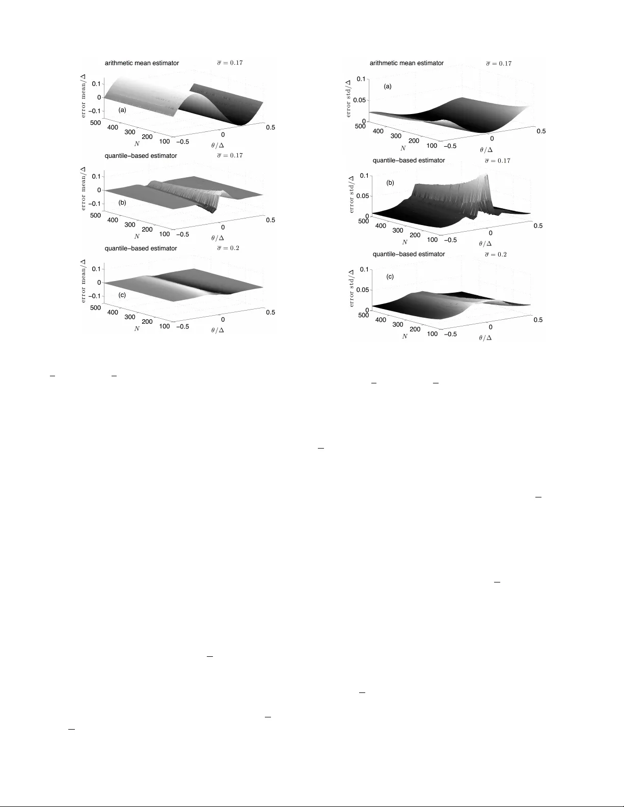
1 P arametric System Identification Using Quantized Data A. Moschitta Member , IEEE and J. Schoukens, F ellow Member , IEEE and P . Carbone Senior Member , IEEE c  2015 IEEE. Personal use of this material is permitted. Permission from IEEE must be obtained for all other uses, in any current or future media, including reprinting/republishing this material for advertising or promotional purposes, creating new collective works, for resale or redistribution to servers or lists, or reuse of any copyrighted component of this work in other works. DOI: 10.1109/TIM.2015.2390833 Abstract —The estimation of signal parameters using quantized data is a recurr ent problem in electrical engineering . As an example, this includes the estimation of a noisy constant value, and of the parameters of a sinewa ve that is its amplitude, initial record phase and offset. Conv entional algorithms, such as the arithmetic mean, in the case of the estimation of a constant, are known not to be optimal in the presence of quantization errors. They provide biased estimates if particular conditions regarding the quantization process are not met, as it usually happens in practice. In this paper a quantile–based estimator is presented that is based on the Gauss–Marko v theorem. The general theory is first described and the estimator is then applied to both DC and A C input signals with unknown characteristics. By using simulations and experimental results it is shown that the new estimator outperforms conventional estimators in both pr oblems, by removing the estimation bias. Index T erms —Quantization, estimation, nonlinear estimation problems, identification, nonlinear quantizers. I . I N T RO D U C T I O N The estimation of signal parameters based on quantized data is a problem of general interest in the area of instrumentation and measurement. Frequently the only available information about a physical phenomenon lies in the sequence of quan- tized data obtained through an Analog–to–Digital Conv erter (ADC) and on information partially av ailable about the input sequence. As an example, the estimation of a Direct Current (DC) value, or of the amplitude and the initial record phase of an Alternate Current (A C) sequence, fall among such problems: samples of the input sequence, possibly noisy , are con verted into digital format for further processing, to identify the needed parameters. As shown in [1]–[5], unless particular conditions apply , the application of conv entional algorithms such as the arithmetic mean or the Least Square Estimator (LSE) result in biased estimates. T ypically , the estimation bias depends on the type of identification problem, e.g. DC or A C type of problem, on the noise Probability Density Function (PDF) and on the ADC characteristics. If the ADC is perfectly uniform, theoretical results can be applied to remove the bias in both the DC and the AC cases, as the quantizer can be linearized on the average. In practice, howe ver , ADCs are not uniform. They rather exhibit Integral (INL) and Differential Nonlinearities (DNL), largely inv alidating the hypotheses re- quired for the application of the theoretical results allo wing simplified signal processing of quantized samples. A. Moschitta is with the Univ ersity of Perugia - Engineering Department, via G. Duranti, 93 - 06125 Perugia Italy , J. Schoukens is with the Vrije Universiteit Brussel, Department ELEC, Pleinlaan 2, B1050 Brussels, Belgium. P . Carbone is with the University of Perugia - Engineering Department, via G. Duranti, 93 - 06125 Perugia Italy . The problem of identifying signal parameters, after noise is added and quantization is performed, can be seen in the larger context of the reconstruction of an input signal PDF: in the DC case the PDF is constant o ver time, in the AC case it becomes time–dependent. When estimating the PDF at the input of a quantizer through the quantized samples, it was prov en in [6] that the follo wing few cases may occur: • if the hypotheses of the quantization theor em hold true, then the input PDF can be reconstructed with no errors; • if the hypotheses of the quantization theorem do not hold true but the noise is Gaussian with a v ariance comparable to the nominal quantization step ∆ , then the input PDF can be reconstructed by using the results of this theorem with some (negligible) errors; • in all other cases, the quantization theorem can not be applied and some other techniques must be used. This occurs, for instance, when the characteristic function of the input PDF is not band–limited, when the input variance is small compared to ∆ , or when the quantizer is not uniform, as it happens frequently in practical cases. When the third case applies, non–subtractive dithering may partly relieve from the bias problem, as it smooths the mean value of the input–output ADC characteristic [4], at the cost of an increased v ariance. Alternati vely , in solving parametric estimation problems related to the input PDF , such as the estimation of the mean of Gaussian noise, a Maximum– Likelihood Estimator (MLE) can be adopted as in [7]–[12]. Howe ver , because of the nonlinearity of the quantizer input– output characteristics, this results in expressions that can be treated only by numerical processing with all practical im- plications: potential con vergence problems, numerical tuning of algorithmic parameters, initialization of the algorithm and local– instead of global–maxima. It is shown in this paper that by using some additional infor - mation, e.g. when the noise PDF is kno wn up to a limited set of parameters, ADC data can be used to obtain accurate estimates of unknown parameters, by using linear identification models applied to suitably pre–distorted output samples. A general approach following this strategy is presented in [13], where the fundamental underlying theory of system identification based on quantized samples, is presented. A similar approach is follo wed in this paper where it is sho wn, both by simulations and experimental results, how to obtain unbiased parametric estimation of the ADC input PDF . With respect to [13] the estimator presented in this paper is based directly on the Gauss–Markov theorem and does not require the introduction of a specific procedure leading to the quasi–con vex combi- nation estimator . Moreover , it estimates the error covariance 2 matrix by av oiding the iterated calculations associated with the recursiv e approach tak en in [14]. Experimental results obtained by using a commercial Data Acquisition System (D AS) prove the validity of the adopted hypotheses on the simplifying assumptions taken in this paper . Its v alidity is also proven here when the noise standard deviation is small compared to ∆ , a typical situation in many cases of practical interest when using ADCs. The approach is general enough to accommodate for generic noise PDFs and when nuisance parameters must be estimated along with the input signal parameter values. T wo typical estimation problems are considered in this paper: • DC case: the estimation of a DC value; • AC case: the estimation of the amplitude, initial record phase and of fset of a sinew ave, when signals are affected by zero–mean Gaussian noise and quantized by a possibly non–uniform ADC. It is sho wn that the presented estimator outperforms the arithmetic mean estimator in the DC case and the LSE in the A C case, by largely removing the estimation bias. This paper is organized as follows. In Section II we in- troduce the considered system, the associated signals and the adopted symbol con ventions. Section III contains the mathe- matical analysis supporting the performance of the quantile– based estimator . It is organized in subsections to address both DC and A C estimation problems with the same modeling approach. Montecarlo–based simulation results are presented in Section IV to v alidate the deri ved theory . Section V contains the description of the experiments done to further prove the estimator properties under the various assumed constraints, while Section VI includes comments on the results sho wn and limits of the proposed estimation procedure. I I . S I G NA L S A N D S Y S T E M S In this Section we illustrate the properties of the quantizing system considered in this paper and the type of input signals applied at its input. The assumed signal chain is depicted in Fig. 1. In this figure, x [ · ; θ ] represents a discrete time deterministic sequence known up to a vector parameter θ and η a zero–mean noise sequence with a giv en PDF and independent outcomes, whose v ariance might be unknown. The quantizer Q ( · ) in Fig. 1 models the effect of the ADC on the signal. It might be non–uniform, but with L kno wn transition le vels, Q ( · ) x [ · ; ✓ ] ⌘ [ · ] y [ · ] Fig. 1. The signal chain considered in this paper . By assuming L as an ev en integer , the quantizer output becomes equal to y k : = −  L 2 − 1  ∆ + k ∆ , k = 0 , . . . , L − 1 (1) when the input takes values in the interval [ T k , T k +1 ) , where T k is the k –th quantizer transition lev el. Accordingly , k = 0 and k = L − 1 correspond to the quantizer output being equal to − ( L / 2 − 1)∆ and L / 2 ∆ , respecti vely . If the transition lev els are unkno wn, they can be estimated during an initial system calibration phase. It will be shown in Section V that the estimator is enough robust to account for uncertainties in the estimated v alues of the transition lev els. It is further assumed that N samples of the ADC output sequence y [ · ] are collected and processed. Consequently , each ADC output sample can be modeled as a random v ariable taking values in L possible categories with probability deter- mined by the deterministic input sequence, the noise PDF and the ADC transition le vels. The additional assumption is made that the quantizer is nev er overloaded, that is the input signal varies in the input range that guarantees the quantization error to be granular . Be- fore describing the proposed estimator, a motiv ating example is gi ven in the next Section. A. A motivating example Assume that x [ n ; θ ] = θ 1 , that is an unknown constant value. The natural and most widely used estimator of θ 1 is the arithmetic mean estimator ˆ θ 1 : = 1 N N − 1 X i =0 y [ i ] . (2) If the ADC is uniform and the noise PDF has suitable prop- erties, e.g. the noise characteristic function is band–limited or appropriate dithering noise is used, ˆ θ 1 is unbiased. In all other situations that most frequently apply in practice, e.g. when the quantizer inside the ADC is non–uniform or when the noise PDF does not satisfy particular conditions, ˆ θ 1 is biased. As an example, assume a 12 -bit ADC uniform in the range [ − 1 , 1) and the noise PDF as a zero–mean Gaussian random sequence with σ = 0 . 25∆ . Under these conditions the bias of (2) is shown in Fig. 2, when N = 50 . Since the expected value of (2) does not actually depend on N , ev en by increasing the number of averaged samples, the bias does not vanish. In the following, it will be sho wn how to remo ve this bias by using an estimator based on a linear model between data and unknown parameters. I I I . Q UA N T I L E – B A S ED E S T I M A T I O N In this Section, at first the main idea behind the proposed estimator is illustrated using a simple example. Then, the parametric signal models are defined and the full estimator is described in the general case. 3 −0.5 0 0.5 −0.1 −0.05 0 0.05 0.1 a r i t h m e t i c m e a n e s t i m a t o r N = 5 0 σ = 0 . 2 5 ∆ θ 1 / ∆ b i a s / ∆ Fig. 2. Arithmetic mean estimator. Bias in the estimation of a DC v alue in Gaussian noise with σ = 0 . 25∆ . A. The estimation of a quantized noisy constant T o show the approach taken in this paper to estimate parametric signals using quantized data, consider the simple problem of estimating a constant in noise using a single–bit quantizer , that is a comparator . Thus, assume x [ n ] = θ + η [ n ] , y [ n ] =  1 x [ n ] ≥ 0 0 x [ n ] < 0 n = 0 , . . . , N − 1 (3) where θ is the constant to be identified, η [ n ] is zero–mean Gaussian noise, having a kno wn variance σ 2 and y [ n ] is the sequence of quantized data. Then simple processing shows that the probability of y [ n ] being positiv e is: p 1 : = P ( y [ n ] = 1) = P ( x [ n ] ≥ 0) = 1 − Φ  − θ σ  (4) T wo aspects can be highlighted: • by collecting data from the comparator , the probability (4) can be estimated by elementary processing; • when the probability p 1 is known, or approximately known, (4) can be in verted to find a value for θ : ˆ θ = − σ Φ − 1 (1 − ˆ p 1 ) (5) where ˆ θ is an estimator of θ and ˆ p 1 an estimator of p 1 . As an example consider the case θ = 0 . 1 , N = 10 1 , . . . , 10 4 . By simple counting the number of times that the comparator outputs equals 1 an estimate of p 1 is obtained. Then θ is estimated as shown in Fig. 3 as a function of N . This approach can be extended to the case of a multi bit quantizer and to different signal models, as done in the next Sections. B. Extension of the pr oposed appr oach to a multi bit quantizer It will be shown that all the estimation problems considered in this paper can be solved by the application of the Gauss– Markov theorem. Accordingly , assume that the sequence of observations X can be linearly related to the unknown param- eters θ as in the following X = H θ + W, (6) where X = [ x 1 x 2 . . . x N ] T represents a column vec- tor containing outcomes of the observable variable, θ = [ θ 1 θ 2 . . . θ M ] T , the column vector with the unknown parameters to be estimated, H is a N × M matrix with kno wn 10 2 10 3 10 4 0.05 0.1 N ˆ θ Fig. 3. Estimate of a constant in noise using (5). Estimator mean value as a function of the number of samples in 10 1 , . . . , 10 4 : the constant to be estimated is θ = 0 . 1 , the noise is zero–mean Gaussian with σ = 0 . 1 . entries and W = [ w 1 w 2 . . . w N ] T , is a column vector containing outcomes of the noise affecting the observable variables. Then, if the noise vector is zero–mean, it can be shown that the Best Linear Unbiased Estimator (BLUE) of θ is [19]: ˆ θ : = ( H T Σ − 1 X H ) − 1 H T Σ − 1 X X, (7) where Σ X represents the covariance matrix of the noise vector W . In the next subsections it is shown how to cast sev eral parametric identification models in the form (6), so to apply (7) for their solution. The added complexity here refers to the ef fect of quantization that correlates outcomes and distorts input data because of its nonlinear input–output characteristic. Thus, each problem considered in the following will be addressed by: • considering the effect of quantization and showing ho w to linearize the relationship between observable data (the quantized output sequence) and unknown parameters, as in (6); • showing that the quantizer output sequence provides useful information for the unbiased estimation of the input noise quantiles; • illustrating how to estimate the noise covariance matrix required by (7), by using available information provided by the quantizer; • using (7) to provide an expression for the estimator in the considered cases. In subsections C–H the idea presented in subsection III-A is extended to comprehend the case of se veral quantization lev- els. At first, the considered DC and A C models are presented in subsection C and then the estimator forms are expressed, by additionally assuming a Gaussian noise PDF . C. The DC and AC parametric signal models In this subsection, the DC and A C data models considered in the follo wing subsections are presented. Assuming n = 0 , . . . , N − 1 , the analyzed DC parametric models are: model 1 : y [ n ] = θ 1 + σ η [ n ] + e [ n ] , model 2 : y [ n ] = θ 1 + θ 2 η [ n ] + e [ n ] , (8) 4 where e [ · ] is the quantization error sequence. While in model 1 the noise standard deviation σ is assumed to be known, in model 2 this is taken as a second parameter to be estimated. The identification of a third A C parametric model, model 3 : y [ n ] = θ 0 + θ 1 x 1 [ n ] + θ 2 x 2 [ n ] + σ η [ n ] + e [ n ] , (9) is considered, where x 1 [ n ] , x 2 [ n ] are known periodic se- quences and θ i , i = 0 , 1 , 2 , are three parameters to be identified. The additional assumption for this model is that sampling is coherent , that is synchr onous and such that N corresponds to an integer number of periods of both x 1 [ · ] and x 2 [ · ] . For instance, if x 1 [ n ] = cos( ω n ) and x 2 [ n ] = sin( ω n ) where ω is a known constant, (9) represents the well known model of the three–parameter sine fit [15]. In the following, the properties of a quantile–based estimat or applied to all these cases will be illustrated. D. The ADC as a Sour ce of Or dinal Data In this subsection, the statistical properties of the sequence of data output by an ADC are recalled, so to serve as a basis for the proposal of a quantile–based estimator . As a general remark, the quantizer inside the ADC maps the input v alues to an ordinal scale that admits calculation of the mean value of the measurement results, as in (2), not without controv ersy 1 . Con versely , generally applicable statistics include the estima- tion of quantiles that will be applied in the follo wing to remov e the potential incongruences associated with the usage of (2). In this subsection an analysis is made on the properties of the information av ailable when solving model 1 through model 3 problem types. For a gi ven value of θ 1 in model 1 and model 2 define, Π = [ p 0 . . . p L − 1 ] T where each p k represents the probability of y [ · ] taking the v alue y k , and C = [ c 0 . . . c L − 1 ] T where c k : = N p k , is the a verage number of occurrences in code bin k when N samples are collected. Also define, C Π = [ cp 0 . . . cp L − 1 ] T where cp k = P k n =0 p n . Moreover define ˆ C = [ˆ c 0 . . . ˆ c L − 1 ] T as the random vector containing the experimental number of occurrences in each code bin and d C Π = [ b cp 0 . . . b cp L − 1 ] T where b cp k : = P k n =0 ˆ c n . Then ˆ C is a random variable having a multinomial distri- bution with parameters N and Π for which [16]: E ( ˆ C ) =    N p 0 . . . N p L − 1    (10) and whose cov ariance matrix is [16]: Σ ˆ C =      N p 0 (1 − p 0 ) − N p 0 p 1 . . . − N p 0 p L − 1 − N p 0 p 1 N p 1 (1 − p 1 ) . . . − N p 1 p L − 1 . . . . . . . . . . . . − N p 0 p L − 1 − N p 1 p L − 1 . . . N p L − 1 p L − 1      (11) 1 As pointed out by [17], even Stevens makes a practical concession to the usage of otherwise not admissible statistics of ordered data [18]: In the strictest pr opriety the ordinary statistics involving means and standar d deviations ought not to be used with these (or dinal) scales, for these statistics imply a knowledge of something more than the relative rank–or der of data. On the other hand, for this ’illegal’ statisticizing ther e can be invoked a kind of pr agmatic sanction: In numer ous instances it leads to fruitful results. Then the maximum likelihood estimator of p k is, ˆ p k = ˆ c k N k = 0 , . . . , L − 1 (12) and ˆ Π = [ ˆ p 0 . . . ˆ p L − 1 ] T is an unbiased estimator of Π with cov ariance matrix Σ ˆ Π = 1 N 2 Σ ˆ C . Observe that regardless of the true value of the sequence generating a given quantized output sequence, when the prob- lem is a static one, the only av ailable information at the quantizer output can be modeled as done in this subsection. Thus, the open problem remains that of exploiting efficiently these data to extract all possible information about the un- known parameter . Moreover , since off–diagonal entries in the cov ariance matrix Σ ˆ C are not null, it is expected that the simple mean estimator of θ 1 will not yield optimal statistical performance, as it ignores both that different v alues have different probability of occurrence and the mutual information carried by different values of the quantized sequence. Alter- nativ e estimators can be employed as shown in the following. E. Model 1 By assuming that the quantizer is not overloaded we have: F y ( y k ) : = P ( y [ n ] ≤ y k ) = P ( θ 1 + σ η [ n ] ≤ T k ) = F  T k − θ 1 σ  = k − 1 X n =0 p n : = cp k , k = 1 , . . . , L − 1 (13) with F ( · ) as the noise cumulati ve distribution function, from which we deri ve T k = F − 1 y ( cp k ) = θ 1 + σ F − 1 ( cp k ) k = 1 , . . . , L − 1 . (14) Since cp k can be estimated using experimental data, (14) is the key equation for the proposal of a quantile–based estimator [13]. While a mathematical form of the estimator could be deriv ed by resorting to the case of a generic noise PDF , the following subsection adds the hypothesis of Gaussian noise to reduce the lev el of abstraction and to increase usability of results. The approach taken in the next subsection under the assumption of model 1 will be then extended in a similar way to comprehend also model 2 and model 3. F . Gaussian case In the Gaussian case, we have F ( x ) = Φ ( x ) , where Φ( · ) is the cumulative distribution function of a standard Gaussian random v ariable, so that from (14) θ 1 = T k − σ Φ − 1 ( cp k ) k = 1 , . . . , L − 1 . (15) that shows that there is a linear relationship between suitably pre–distorted cumulative probabilities defined in (13), and the constant input θ 1 . T o derive an e xpression for the estimator of θ 1 , cp k will be substituted by ˆ cp k . Accordingly , define L = 5 { k 1 , . . . , k Λ } as the set of indices in the interval 0 , . . . , L − 1 for which 0 < ˆ p k < 1 and Λ ≥ 1 its cardinality and H 1 : = [ Λ z }| { 1 · · · 1] T X 1 : =  T k 1 − σ Φ − 1 ( b cp k 1 ) · · · T k Λ − σ Φ − 1 ( b cp k Λ )  T W 1 : = X 1 − H 1 θ 1 , (16) where W 1 is a noise vector having cov ariance matrix Σ X 1 . The estimation problem can then be written in matrix form: X 1 = H 1 θ 1 + W 1 (17) When N is sufficiently large, the v ariance of b cp k is sufficiently small to allo w usage of a first–order T aylor series expansion of each component in X 1 about E ( b cp k ) = cp k . As a con- sequence, the nonlinear function Φ − 1 ( · ) is linearized so that E ( W 1 ) ' 0 results and (17) satisfies the hypotheses of the Gauss–Markov theorem. Accordingly , the BLUE of θ 1 can be written as [19]: ˆ θ GM 1 : = ( H T 1 Σ − 1 X 1 H 1 ) − 1 H T 1 Σ − 1 X 1 X 1 (18) with V ar  ˆ θ GM 1  = ( H T 1 Σ − 1 X 1 H 1 ) − 1 (19) where Σ X 1 also represents the cov ariance matrix of X 1 . An estimate for the cov ariance matrix of X 1 is obtained by observing that: Σ X 1 = σ 2 Σ Y , (20) where Y =  Φ − 1 ( b cp k 1 ) · · · Φ − 1 ( b cp k Λ )  T and Σ Y its co- variance matrix. An approximated expression for Σ Y can be obtained by linearizing the nonlinear function Φ − 1 ( · ) using a T aylor series expansion about the mean value of each component in d C Π , so that we can write [20]: Σ Y ' J Σ c C Π J T , (21) where J is a diagonal matrix defined as J = diag d Φ − 1 ( x ) dx     x = b cp k 1 , . . . , d Φ − 1 ( dx ) dx     x = b cp k Λ ! . (22) By recalling that the deriv ativ e of the in verse function can be expressed in terms of the deriv ative of the direct function, we hav e: d Φ − 1 ( x ) dx     x = b cp k = 1 d Φ( x ) dx    x =Φ − 1 ( b cp k ) = √ 2 π e 1 2 ( Φ − 1 ( b cp k ) ) 2 k = k 1 , . . . , k Λ (23) Finally , an estimate of the co variance matrix of d C Π to be substituted in (21), can be obtained by observing that C Π = A Π where A =      1 0 · · · 0 1 1 · · · 0 . . . . . . · · · . . . 1 1 · · · 1      (24) is a lower diagonal matrix. Thus the covariance matrix of d C Π is Σ c C Π = A Σ ˆ Π A T , (25) and estimates of Σ ˆ Π and Σ c C Π are obtained by replacing each entry in (11) of the type N p i p j , by the corresponding natural estimator based on the product of estimated probabilities N ˆ p i ˆ p j , with ˆ p i defined in (12). Once all unkno wn quantities are substituted by their estimates in (18), a similar estimator to that presented in [13] (e.g. eq. 6.19) is obtained. G. Model 2 By considering model 2 under the hypothesis of Gaussian noise, the equi valent expression for (14) is: T k = F − 1 y ( cp k ) = θ 1 + θ 2 F − 1 ( cp k ) k = 1 , . . . , L − 1 (26) from which, using the Gaussian hypothesis, we have: T k θ 2 − θ 1 θ 2 = Φ − 1 ( cp k ) k = 1 , . . . , L − 1 . (27) T o linearize the relationship between parameters and observed data, define a new vector parameter γ : = [ γ 1 γ 2 ] T : = h 1 θ 2 θ 1 θ 2 i T . Observe that if an estimate for γ is av ailable, an estimate for θ 1 and θ 2 is easily obtained by inv erting the relationship in the definition of γ . Thus (27) can be rewritten as: T k γ 1 − γ 2 = Φ − 1 ( cp k ) k = 1 , . . . , L − 1 . (28) Then again define L = { k 1 , . . . , k Λ } as the set of indices in the interval 0 , . . . , L − 1 for which 0 < ˆ p k < 1 , Λ ≥ 2 its cardinality and H 2 : =      T k 1 − 1 T k 2 − 1 . . . . . . T k Λ − 1      X 2 : =  Φ − 1 ( b cp k 1 ) · · · Φ − 1 ( b cp k Λ )  T W 2 : = X 2 − H 2 γ , (29) where W 2 is a noise vector having cov ariance matrix Σ X 2 = Σ Y . The estimation problem can then be written in matrix form: X 2 = H 2 γ + W 2 (30) Again, when N is sufficiently large, each component in X 2 can be linearized about the corresponding mean value as in the case of model 1 and E ( W 2 ) ' 0 results. The application of the Gauss–Marko v theorem provides: ˆ θ GM 2 : = ( H T 2 Σ − 1 X 2 H 2 ) − 1 H T 2 Σ − 1 X 2 X 2 (31) with V ar  ˆ θ GM 2  = ( H T 2 Σ − 1 X 2 H 2 ) − 1 (32) where Σ X 2 also represents the covariance matrix of X 2 and is estimated as in the case of model 1. 6 H. Model 3 The coherency condition on sampling implies that an integer number N of periods of x 1 [ · ] and x 2 [ · ] are observ ed. Let us further assume that each period contains M samples of the input signal. Consequently , the total number of samples is K = M N and if the noise η [ · ] would not be present, the quantizer output would be periodic with the same period P = M T S of the known sequences, with T S as the sampling period. By recalling that any real number x can be expressed as the sum of its integer part b x c and of its fractional part h x i we can write x i [ n ] = x i hj n M k M + D n M E M i = x i hD n M E M i i = 1 , 2 , where the equality follo ws by the periodicity assumption. Thus, there are only M different time instants modulo M asso- ciated with n = 0 , . . . , M − 1 , each one recorded N times, that is the number of periods. This is made clear in Fig. 4 where a sinusoidal sequence x 1 [ n ] is assumed with M = 5 and N = 9 . Therefore a total of K = 45 samples is collected, of which only 5 refer to independent time instants. Dashed rectangles in this figure show the samples that provide the same signal amplitude, when the effects of noise and quantization are neglected. No w consider a given v alue of n ∈ { 0 , . . . , M − 1 } and m ∈ I n = : { n, n + M , n + 2 M , . . . , n + ( N − 1) M } . Since, for some integer i , D m M E M =  n + iM M  M = D n M E M = n M M = n for m ∈ I n we can write y [ m ] = θ 0 + θ 1 x 1 [ n ] + θ 2 x 2 [ n ] + σ η [ m ] + e [ m ] , (33) that provides N realizations of the quantizer output for any single value of the constant input θ 0 + θ 1 x 1 [ n ] + θ 2 x 2 [ n ] . Thus, I 0 , . . . , I M − 1 provide a partition of the K samples. Moreover , for a giv en value n , (33) provides N values that can be used to build a histogram of the quantized output, ˆ C [ n ] = [ ˆ c 0 [ n ] . . . ˆ c L − 1 [ n ]] T (34) as the random vector containing the experimental number of occurrences in each code bin when the deterministic input is s [ n ] : = θ 0 + θ 1 x 1 [ n ] + θ 2 x 2 [ n ] and, d C Π[ n ] = [ b cp 0 [ n ] . . . b cp L − 1 [ n ]] T where b cp k [ n ] : = P k n =0 ˆ c n [ n ] . By considering model 3 under the hypothesis of Gaussian noise, the equi valent expression for (14) is: F y ( y k ) : = P ( y [ n ] ≤ y k ) = P ( θ 0 + θ 1 x 1 [ n ] + θ 2 x 2 [ n ] + σ η [ n ] ≤ T k ) =Φ  T k − θ 0 − θ 1 x 1 [ n ] − θ 2 x 2 [ n ] σ  = k − 1 X h =0 p h [ n ] : = cp k [ n ] , k = 1 , . . . , L − 1 (35) where p h [ n ] represents the probability that y [ m ] takes the value h when the input signal is s [ n ] . Thus, from (35) we hav e: θ 0 + θ 1 x 1 [ n ] + θ 2 x 2 [ n ] = T k − σ Φ − 1 ( cp k [ n ]) k = 1 , . . . , L − 1 n = 0 , . . . , M − 1 (36) For each n , define a corresponding set L [ n ] as the set of indices in the interv al 0 , . . . , L − 1 for which 0 < ˆ p k [ n ] < 1 and Λ[ n ] its cardinality . Then define θ 3 : = [ θ 0 θ 1 θ 2 ] T H 3 [ n ] : =      1 x 1 [ n ] x 2 [ n ] 1 x 1 [ n ] x 2 [ n ] . . . . . . . . . 1 x 1 [ n ] x 2 [ n ]      X 3 [ n ] : =      T 1 − σ Φ − 1 ( b cp 1 [ n ]) T 2 − σ Φ − 1 ( b cp 2 [ n ]) . . . T Λ[ n ] − σ Φ − 1 ( b cp Λ [ n ])      W 3 [ n ] : = X 3 [ n ] − H 3 [ n ] θ 3 . (37) Then, an estimate of the cov ariance matrix of W 3 [ n ] is Σ W 3 [ n ] : = σ 2 Σ Y [ n ] , where Σ Y [ n ] is based on the definition in (21), in which each occurrence of b cp k is substituted by b cp k [ n ] . Finally , the matrices for the entire set of M time–dependent input v alues are constructed by defining: H 3 : =  H 3 [0] T · · · H 3 [ M − 1] T  T X 3 : =  X 3 [0] T X 3 [1] T · · · X 3 [ M − 1] T  T Σ X 3 : = diag (Σ W 3 [0] , . . . , Σ W 3 [ M − 1]) T (38) Then the application of the Gauss–Markov theorem provides: ˆ θ GM 3 : = ( H T 3 Σ − 1 X 3 H 3 ) − 1 H T 3 Σ − 1 X 3 X 3 (39) with V ar  ˆ θ GM 3  = ( H T 3 Σ − 1 X 3 H 3 ) − 1 (40) Observe that: • if for some n , a single quantization bin is excited by the corresponding quantizer input sample, then H 3 [ n ] in (37) vanishes, it must be discarded and not included in the dataset used to form H 3 in (38); • enough information is needed to estimate the 3 scalar parameters in θ 3 , that is the number of ro ws of H 3 in (38) must be not less than 3 . In the two following Sections both simulation and experimen- tal results are presented. 0 5 10 15 20 25 30 35 40 45 −1 −0.5 0 0.5 1 Fig. 4. Model 3. Sinewav e coherent sampling in absence of additive noise and quantization: N = 9 periods of the sinusoidal signal having each M = 5 samples per period. N independently sampled values are obtained that are periodic with period M . 7 Fig. 5. Model 1. Mean value of the estimation error of a quantized constant in noise normalized to ∆ . Montecarlo results based on 5000 records as a function of θ / ∆ and N : arithmetic mean estimator (a), quantile–based estimator when σ = 0 . 17 (b) and σ = 0 . 2 (c). I V . S I M U L A T I O N R E S U LT S At first model 1 was considered. Mean values and standard deviations of the estimation errors obtained by the Montecarlo approach based on R = 5000 records are presented in Fig. 5 and in Fig. 6, respectiv ely , as a function of both θ / ∆ and N = 100 , . . . , 500 . All results were obtained assuming ∆ = 2 / 2 b , where b = 10 is the number of bits, and were normalized with respect to ∆ . Given the periodic behavior of the quantization error input–output characteristic, curves in Fig. 5 and Fig. 6 are periodic with ∆ and their behavior is shown here, assuming the single period − ∆ / 2 < θ < ∆ / 2 . The estimation mean error is plotted in Fig. 5 in the case of the simple arithmetic mean (a) and in the case of the quantile–based estimator (b-c). While the simple arithmetic mean estimation error does not depend on N , the performance of the newly proposed estimator also depends on the number of av eraged samples. This is a common behavior in the case of bias–removing procedures [23]. In both cases, the mean square error decreases when increasing the number of processed samples. Fig. 5(c) shows that already with σ = 0 . 2 the estimation bias is largely removed in comparison to results shown in Fig. 5(a). Fig. 6 shows the behavior of the normalized standard deviation of the estimation error . Fig. 6(a) refers to the arithmetic mean estimator while Fig. 6(b) and Fig. 6(c) show the normalized standard deviation of ˆ θ GM 1 when σ = 0 . 17 and σ = 0 . 2 , respectively . Results show that in all cases the standard deviation remains of the same order of magnitude, with the newly proposed estimator removing the largest part Fig. 6. Model 1. Standard deviation of the estimation error of a quantized constant in noise normalized to ∆ . Montecarlo results based on 5000 records as a function of θ / ∆ and N : arithmetic mean estimator (a), quantile–based estimator when σ = 0 . 17 (b) and σ = 0 . 2 (c). of the estimation bias. Thus, the new estimator removes the bias at the expense of an increased variance. Since when σ > 0 . 4 , the arithmetic mean already sho ws negligible bias when the noise is Gaussian [1], the quantile–based estimator is more effecti ve when the noise standard deviation is lower than this bound. Con versely , both estimators tend to provide similar results. Moreov er , observe that already for σ = 0 . 2 , the normalized standard deviation of ˆ θ GM 1 approximately achiev es the square–root of the Cramer–Rao lower bound applicable to unbiased estimators of a quantized constant in Gaussian noise with kno wn v ariance [9]. This becomes e vident in Fig. 7 where both the normalized estimator variance and the corresponding Cramer–Rao lower bound are plotted as a function of θ / ∆ , assuming N = 300 and σ = 0 . 2 . While the two curves tend to coincide when | θ/ ∆ | ' 0 . 5 , the small positiv e and negati ve dif ferences for other values of θ / ∆ are due to the residual estimator bias. Thus, the proposed estimator is capable to be statistically ef ficient under suitable values of its tuning parameters. When model 2 is considered, the bias of the arithmetic mean estimator and that associated with the quantile–based estimator are shown in Fig. 8(a) and (b), respecti vely . The noise standard deviation σ = 0 . 34 was assumed which results in an overall lower bias for the arithmetic mean estimator and its remov al by the quantile–based estimator already when N is slightly larger than 100 . Consider howe ver that model 2 can be reduced to model 1 if the known value of the noise standard deviation is substituted by an estimate of it obtained using alternative 8 −0.5 0 0.5 0.01 0.02 0.03 0.04 θ / ∆ s t d 1 ˆ θ G M 1 2 / ∆ √ C R L B / ∆ Fig. 7. Model 1. Comparison between the normalized standard deviation of ˆ θ GM 1 obtained as in Fig. 6 and the corresponding Cramer–Rao lower bound for unbiased estimators, deriv ed using an expression published in [9]. estimators as in [15][21]. Simulations were also done when assuming model 3. Re- sults are plotted in Fig. 9, based on 1000 Montecarlo records. This figure shows the av erage residual error in the estimation of s [ · ] based on 1000 records, when assuming x 1 [ n ] = cos  2 π n M N  and x 2 [ n ] = sin  2 π n M N  , with M = 20 samples per period, N = 50 periods and θ ∆ = [3 . 7 11 . 4 23 . 1] . A 10 bit quantizer is considered having ∆ = 2 / 2 10 and being affected by Gaussian noise with σ = 0 . 3∆ . For each time index m , the mean value of the difference between the simulated and estimated sinewa ves is plotted in this figure. T o prov e the validity of the new approach, the known quantization lev els were assumed affected by INL uniformly distributed in ( − ∆ / 2 , ∆ / 2) . Both the errors associated with the usage of the proposed estimator (bold line) and of the well–known least– square estimator (thin line) are sho wn. The inset shows an enlarged view of the first 100 samples. Data in Fig. 9 show that the ne w estimator is capable of reducing the estimation bias and improving estimation accu- racy . The new estimator requires kno wledge of the transition lev el values, while the least–square estimator does not. While a calibration phase might be required in those cases where the ADC can not be considered to be linear enough, this additional information is exploited by the algorithm to improv e estimation accuracy . Con versely , the least–square estimator does not include this information and its performance degrades progressiv ely when the ADC behavior departs from ideality . V . E X P E R I M E N TA L R E S U LT S T o prove the practical viability of the proposed estimator, the signal chain depicted in Fig. 10 was used. A 12 –bit commercial DAS with ∆ = 0 . 005085 V was used to prove the applicability of the proposed estimators. The transition lev els of the DAS, as defined in [15], were first estimated, along with the D AS noise standard de viation ˆ σ DAS ' 0 . 15∆ , measured as of clause 9.4.2 in [15]. The D AS was also calibrated for offset errors by simple pre–processing of all acquired data: raw data were multiplied by a gain and added to a constant value to remove offset and the gain errors [15]. Three sets of experiments were performed to test the proposed estimator under the hypotheses of model 1 and model 3. Fig. 8. Model 2. Mean value of the estimation error of a quantized constant in noise normalized to ∆ (model 1). Montecarlo results based on 5000 records as a function of θ / ∆ and N , when σ = 0 . 34 : arithmetic mean estimator (a), quantile–based estimator (b). A. Model 1 assumption: experimental results A wa veform synthesizer used as a source of DC voltages affected by artificially added Gaussian noise, with noise stan- dard de viation σ η , was used to provide input v alues to the 200 400 600 800 1000 −0.1 −0.05 0 0.05 m e a n r e s i d u a l e r r o r / ∆ m 20 40 60 80 100 Fig. 9. Model 3. Mean value of the estimation error normalized to ∆ , as a function of the sampling index: the Gauss–Markov estimator (bold line) and the least–square estimator (thin line). Simulations were based on 1000 Montecarlo records, known sequences x 1 [ · ] and x 2 [ · ] and σ = 0 . 3∆ , with ∆ = 2 / 2 10 . DMM FLUKE 8845A WA VEFORM SYNTHESIZER AGILENT 33220A PC DA T A ACQUISITION BOARD NI 6008 ETHERNET USB Fig. 10. Measurement setup used to collect experimental data. 9 −15 −10 −5 0 5 10 15 −0.2 0 0.2 e r r or m e a n / ∆ θ / ∆ Fig. 11. Model 1. Mean value of the estimation error of a quantized constant in noise normalized to ∆ . Experimental results obtained using the setup shown in Fig. 10. and N = 500 . Estimator bias as a function of θ / ∆ when using the arithmetic mean estimator (solid line) and the quantile–based estimator (dots). For each θ / ∆ a single record of N = 500 was used. Transition levels and input–referred noise standard deviation are first estimated using experimental data, for model 1 to be applicable (see text). 3.5 4 4.5 5 5.5 6 6.5 0 0.02 0.04 0.06 0.08 0.1 L S - a l g or i t h m q u a nt i l e –b a s e d a l g or i t h m e r r or m e a n / ∆ s i n e a m p l it u d e / ∆ Fig. 12. Model 3. Mean value of the estimation error of the amplitude of a synchronously sampled sinewa ve normalized to ∆ , based on 5 records of 8000 points each. Experimental results obtained using the setup shown in Fig. 10. Estimator bias as a function of 100 sinewa ve amplitude in the interval (0 . 05 , 0 . 1) V , when using the least–square estimator (solid line) and the quantile–based estimator (stars). ADC transition lev els, whose value is shown using dashed lines, and input–referred noise standard de viation are first estimated using experimental data, for model 3 to be applicable (see text). D AS, in the range ( − 19∆ , 19∆) V . The total measured noise standard deviation σ ' ( σ 2 η + σ 2 DAS ) 1 / 2 , comprehensiv e of the D AS input–referred contribution, was estimated during the calibration phase as ˆ σ ' 0 . 264∆ . A 6 1 / 2 –digit digital multimeter (DMM) was employed to measure a true quantity value of the DAS input [22]. For each of the 800 DC values in the input range a single record of N = 500 acquisitions was collected by the DAS, along with the reference value measured by the DMM. All instruments were connected to a PC using either the Ethernet or a USB connection. Data were processed to obtain estimates of the applied DC value and of the corresponding estimation errors. Both the simple mean value estimator and the newly proposed estimator were used, under the assumptions of model 1. Results are plotted in Fig. 11 using a solid line and dots, in the former and latter case, respectively . They confirm the accuracy of the proposed procedure and show that it is ef fective in removing the estimation bias characterizing the simple mean estimator . B. Model 3 assumption: experimental results A waveform synthesizer was used to generate a 100 Hz sinew av e with 100 variable amplitudes in the range (0 . 05 , 0 . 1) V , without the addition of noise. This signal was acquired by the DAS sampling at 10 4 ksample/s, providing M = 100 samples per period. For each one of the 100 voltage values, 8000 points resulting in N = 80 periods, were recorded and processed using both the standard least–square method described in [15] and the newly proposed quantile–based estimator to estimate θ 1 , θ 2 , θ 3 . The sinew av e amplitude was then estimated as q ˆ θ 2 1 + ˆ θ 2 2 , with ˆ θ i , i = 1 , 2 as each one of the two estimators. The amplitude reference value was measured by the DMM put in AC mode, as the mean value of 10 measurement results. The mean error obtained using 5 records for each sinew av e amplitude is plotted in Fig. 12 in both cases, using a solid line for the LS–estimator and stars for the newly proposed estimator . Given that only the sine wav e amplitude is estimated, there was no need to synchronize the D AS with the wav eform synthesizer . Thus, the initial record phase of the sinewa ve generator was not controlled and was assumed as a uniform random v ariable in [0 , 2 π ) . V I . D I S C U S S I O N O F R E S U LT S In this Section, at first general properties of the proposed estimator are discussed on the basis of the described results. Then, kno wn estimator issues and corresponding fixes are examined. A. P erformance comparison The proposed estimator can be used to obtain accurate measurements of parameters of DC and A C sequences if some of the characteristic parameters of the D AS used to quantize data are known, such as transition le vels and input–referred noise standard de viation. Eventual errors in the estimation of these parameters performed beforehand, will not affect significantly the performance of the estimator , as shown by data in Fig. 11 and 12. If nominal thresholds values are used instead of actual values, the estimator still provides reasonable results, improving over the performance of the simple mean estimator . Provided that the noise standard deviation is large enough to excite a number of quantization bins exceeding at least by one the number of parameters to be estimated, there are no restrictions on the sev erity of the applied quantization: accurate estimates are obtained e ven when data are quantized using lo w–resolution D ASs. In practice, the effect of noise is that of encoding the information about the unknown parameters’ values in the probabilities with which the v arious quantizer output codes occur . The algorithm presented here acts as a decoder of such information, by properly processing the estimated probabili- ties. Moreover , while the usual approach to process quantized data is based, at most, on calibration of ADCs for offset and gain, the presented estimator allo ws calibration at the transition lev el and is thus inherently more statistically po werful. Finally , the same approach followed here can be applied with noise PDFs different from the Gaussian one, by recalculating the cov ariance matrix and by using the proper quantile equation in (15) and in (27). 10 −0.1 −0.05 0 0.05 0.1 0 2 4 6 x 10 −3 θ / ∆ m s e / ∆ 2 quantile based estimator arithmetic mean estimator Fig. 13. Model 1. Mean–square error in the the estimation of a quantized constant in noise normalized to ∆ 2 . Montecarlo results based on 1000 records of N = 1000 samples each, as a function of θ / ∆ , when σ = 0 . 2 . B. Known issues and fixes It is not assured that the quantile–based estimator uniformly outperforms other estimators. For instance, consider the case shown in Fig. 13, where the mean–square error is plotted, under model 1, for both the quantile–based and the arith- metic mean estimators. Here, N = 1000 is assumed and 1000 records of θ varying in the interval [ − 0 . 1∆ , 0 . 1∆] are considered. By knowing that the closest transition lev els are positioned in − ∆ / 2 and ∆ / 2 , it can be observed that when θ ' 0 the quantile–based estimator maintains its overall behavior . Con versely , the arithmetic mean estimator benefits from the DC level getting close to an ADC equiv alent output lev el ( ' 0 ) and thus outperforms the quantile–based estimator . Moreov er , the proposed quantile–based estimator may fail when the record length N is so small or σ  1 , so that all samples in the record belong to the same quantization bin. This results in a situation where all collected samples excite the same bin that would be excited if the noise would not be present. Under model 1 this results in Λ = 0 and the estimator not having enough information to identify the model. In a similar way model 2 and model 3 may not be identifiable if Λ drops below 2 and 3 , respectively . These ev ents are unlikely if N  1 and/or σ > 1 / 6 . Howe ver , an easy fix could be proposed by resorting to a mechanism that recognizes the occurrence of such phenomena and switches to more con ventional estimators, such as the LSE or the MLE. V I I . C O N C L U S I O N An estimator is presented in this paper that exploits the unbiasedness of a quantile estimator based on ADC output data, when the quantile le vel coincides with the value of one of the ADC transition lev els. The estimator is based on a linear relationship between a statistics of the observed data using nonlinear functions and parameters to be identified, and is thus easily computable using matrix calculations. By also taking into account the covariance between the ADC output codes, it was possible to show that this estimator is an application of the Gauss–Marko v theorem and that it is rather robust tow ard inaccuracies in some of the necessary hypotheses. A C K N O W L E D G E M E N T This work was supported in part by the Fund for Scientific Research (FWO-Vlaanderen), by the Flemish Government (Methusalem), the Belgian Government through the Inter univ ersity Poles of Attraction (IAP VII) Program, and by the ERC adv anced grant SNLSID, under contract 320378. R E F E R E N C E S [1] P . Carbone, “Quantitative criteria for the design of dither-based quan- tizing systems, ” IEEE T rans. Instr . Meas. , vol. 46, no. 3, pp. 656–659, June 1997. [2] I. Koll ´ ar , “Bias of mean v alue and mean square v alue measurement based on quantized data, ” IEEE T rans. Instr . Meas. , vol. 43, pp. 373–379, Oct. 1994. [3] L. Schuchman, “Dither signals and their effect on quantization noise, ” IEEE Transaction on Communication T echnology, vol. 12, pp. 162–165, 1964. [4] R. M. Gray , T . G. Stockham, “Dithered Quantizers, ” IEEE T rans. Inform. Theory , V ol. 39, no. 3, May 1993, pp. 805–812. [5] R. M. Gray , D. L. Neuhoff, “Quantization, ” IEEE T rans. Inform. Theory , V ol. 44, no. 6, Oct. 1998, pp. 2325–2383. [6] B. W idrow and I. Koll ´ ar , Quantization Noise , Cambridge University Press, 2008. [7] A. Di Nisio, L. Fabbiano, N. Giaquinto, M. Savino “Statistical Properties of an ML Estimator for Static ADC T esting, ” Proc. of 12th IMEKO W orkshop on ADC Modelling and T esting, Iasi, Romania, Sept. 19–21, 2007. [8] Y . Gendai, “The Maximum–Likelihood Noise Magnitude Estimation in ADC Linearity Measurements, ” IEEE T rans. Instr . Meas. , July 2010, vol. 59, no. 1, pp. 1746–1754. [9] A. Moschitta, J. Schoukens, P . Carbone, “Information and Statistical Efficienc y When Quantizing Noisy DC V alues, ” accepted for publication in IEEE T rans. Instr . Meas. . [10] L. Balogh, I. Koll ´ ar , L. Michaeli, J. ˇ Saliga, J. Lipt ´ ak, “Full information from measured ADC test data using maximum likelihood estimation, ” Measur ement , vol. 45, pp. 164–169, 2012. [11] J. ˇ Saliga, I. K oll ´ ar , L. Michaeli, J. Bu ˇ sa, J. Lipt ´ ak, T . V irosztek, “ A comparison of least squares and maximum likelihood methods using sine fitting in ADC testing, ” Measurement , vol. 46, pp. 4362–4368, 2013. [12] F . Gustafsson, R. Karlsson, “Generating dithering noise for maximum likelihood estimation from quantized data, ” Automatica , V ol. 49, pp. 554–560, 2013. [13] L. Y . W ang, G. G. Y in, J. Zhang, Y . Zhao, System Identification with Quantized Observations, Springer Science, 2010. [14] L. Y . W ang and G. Y in, “ Asymptotically efficient parameter estimation using quantized output observations, ” Automatica , V ol. 43, 2007, pp. 1178–1191. [15] IEEE, Standard for T erminology and T est Methods for Analog–to– Digital Converter s , IEEE Std. 1241, Aug. 2009. [16] M. Evans, N. Hastings, B. Peacock, Statistical Distributions – 3rd ed. . W iley , New Y ork, USA 2000. [17] T . R. Knapp, “Treating Ordinal Scales as Interval Scales: An Attempt T o Resolve the Controversy , ” Nursing Resear ch , March/April, vol. 39, no. 2, 1990. [18] S. S. Stevens, “On the Theory of Scales of Measurement, ” Science , vol. 103, no. 2684, June 1946. [19] S. M. Kay , Fundamentals of Statistical Signal Pr ocessing, Prentice–Hall, 1998. [20] K. O. Arra, “ An Introduction T o Error Propagation: Deriv ation, Mean- ing and Examples of Equation C Y = F X C X F T X , ” T echnical Re- port , Swiss Federal Institute of T echnology Lausanne, 1998. [online] http://www .nada.kth.se/˜kai-a/papers/arrasTR-9801-R3.pdf. [21] IEEE, Standard for T erminology and T est Methods for W aveform Digi- tizers , IEEE Std. 1057, Aug. 2007. [22] JCGM 200:2012, International vocabulary of metr ology – Basic and general concepts and associated terms, 3r d ed. , (VIM), ISO, BIPM, IEC, IFCC, ISO, IUP A C, IUP AP and OIML, 2012. [online] http://www .bipm.org/utils/common/documents/jcgm/JCGM 200 2012.pdf. [23] P . Carbone, G. V andersteen, “Bias Compensation When Identifying Static Nonlinear Functions Using A veraged Measurements, ” IEEE T rans. Instr . Meas. , 2014.