Network Detection Theory and Performance

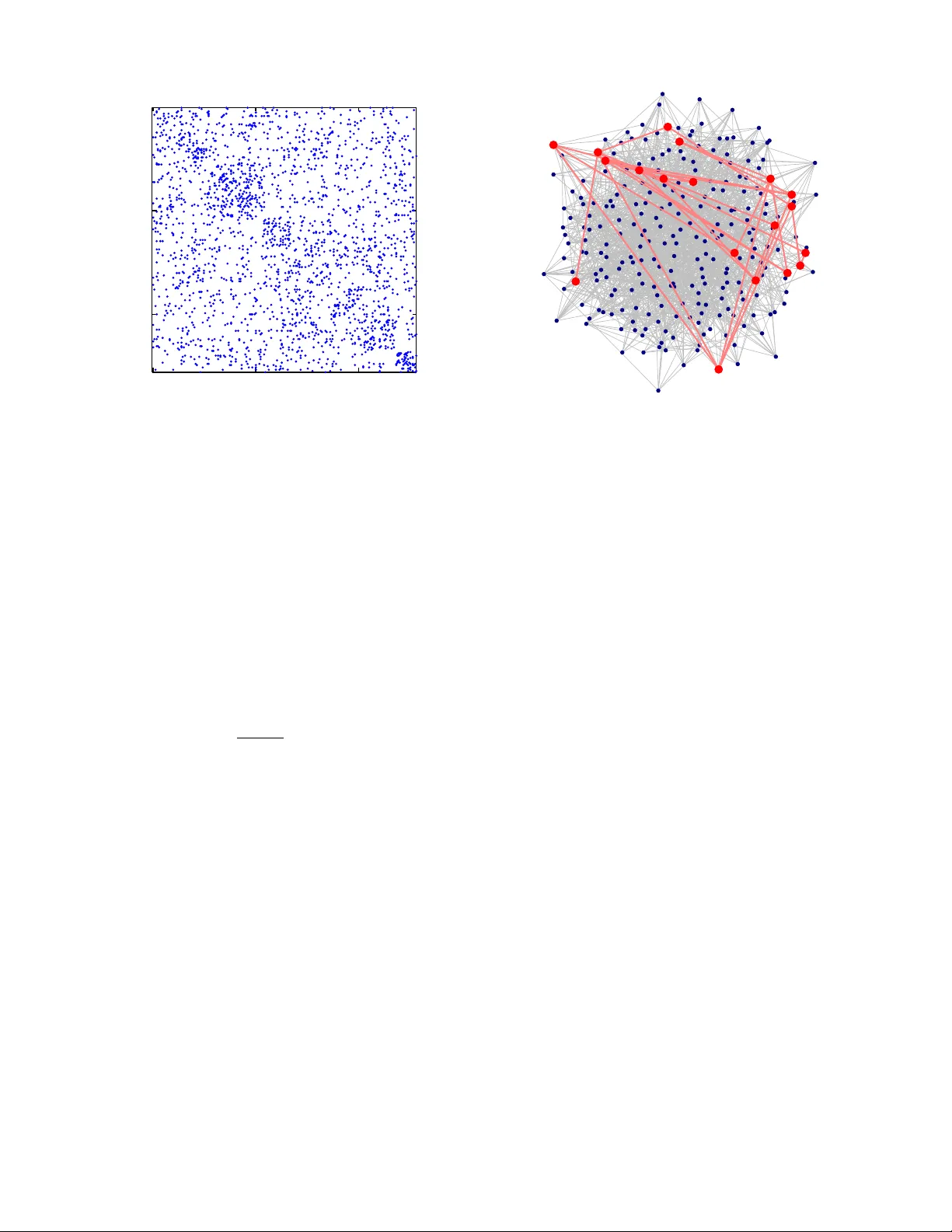
SMITH ET AL.: NETWORK DETECTION 1 Network Detection Theory and Performance Ste ven T . Smith*, Senior Member , IEEE , Kenneth D. Senne*, Life F ellow , IEEE , Scott Philips*, Edward K. Kao* † , and Garrett Bernstein* Abstract —Network detection is an important capability in many areas of applied research in which data can be repr esented as a graph of entities and relationships. Often- times the object of interest is a relatively small subgraph in an enormous, potentially uninter esting background. This aspect characterizes network detection as a “big data” problem. Graph partitioning and network discovery hav e been major resear ch ar eas over the last ten years, driv en by interest in internet sear ch, cyber security , social networks, and criminal or terrorist activities. The specific problem of network discovery is addressed as a special case of graph partitioning in which membership in a small subgraph of interest must be determined. Algebraic graph theory is used as the basis to analyze and compare different network detection methods. A new Bayesian network detection framework is introduced that partitions the graph based on prior information and direct observations. The new approach, called space-time threat propagation, is proved to maximize the probability of detection and is theref ore optimum in the Neyman-Pearson sense. This optimality criterion is compared to spectral community detection approaches which divide the global graph into subsets or communities with optimal connectivity properties. W e also explore a new generative stochastic model for covert networks and analyze using r eceiv er operating character - istics the detection performance of both classes of optimal detection techniques. I . I N T R O D U C T I O N Network detection is a special class of the more general graph partitioning (GP) problem in which the binary decision of membership or non-membership for each graph verte x must be determined. This detection problem and more generally GP are of fundamental and practical importance in graph theory and its applications (Figure 1). The detected subgraph comprises all vertices Manuscript recei ved 2013. *MIT Lincoln Laboratory , Lexington, MA 02420; { stsmith, senne, garrett.bernstein } @ll.mit.edu, edwardkao@fas.harv ard.edu † Department of Statistics, Harv ard Uni versity; Cambridge MA USA 02138 *This work is sponsored by the Assistant Secretary of Defense for Research & Engineering under Air Force Contract F A8721-05- C-0002. Opinions, interpretations, conclusions and recommendations are those of the author and are not necessarily endorsed by the United States Go vernment. declared to be members. The very definition of member- ship will lead to specific network detection algorithms. Graph partitioning is an NP-hard problem; howe ver , semidefinite programming (SDP) relaxation applies to many cases, of fering both practical and oftentimes the- oretically attractiv e approximation to GP . [32], [56] In general, practical GP approaches exploit a variety of global and local connecti vity properties to divide a graph into many subgraphs. Decreasing algorithmic comple xity is achieved in certain domains that may be cast as quadratic optimization problems (yielding eigen v alue- or spectral-based methods), or simple sets of linear equations. One important network detection approach, called community detection, divides the global graph into subsets or communities based on optimizing a specific connectivity measure that is chosen depending upon the application. This paper presents a new Bayes- ian network detection approach called space-time threat propagation [40], [47] that is shown to optimize the probability of network detection in a Ne yman-Pearson sense gi ven prior information and/or direct observ ations, i.e. detection probability is maximized gi ven a fixed false alarm a.k.a. false positi ve probability . This is an important property because it provides a practical op- timum algorithm in many settings (satisfying a set of assumptions detailed later in the paper), and it provides a performance bound on detection performance. Remark- ably , the two apparently dif ferent optimal network detec- tion approaches are related to each other using insights from algebraic graph theory . Conv erse to other research on network detection, rather than using the network to detect signals, [3], [10], [27] the signal of interest in this paper is the signal to be detected. In this sense the paper is also related to work on so-called manifold learning methods, [5], [8], [12] although the network to be detected is a subgraph of an existing network, and therefore the methods described here belong to a class of network anomoly detection [8] as well as maximimum- likelihood methods for network detection. [17] Both spectral-based and Neyman-Pearson network detection methods are described and analyzed below in Sections III and IV. Furthermore, network detection performance is assessed using a ne w stochastic blockmodel [2] for small, dynamic foreground networks embedded within a 2 SMITH ET AL.: NETWORK DETECTION SDP/LP Spectral/SVD/PCA Av = λ v Laplacian Lv = 0 Global Netw orks Local Netw orks • Normalized cut / Conductance • Maximum fl o w • Gr aph partitioning – Latent Semantic Indexing (LSI) – k -means clustering • Gr aph detection – Spectr al partitioning • Multiresolution methods (MR) • Manifold learning (ML) • Community detection • Heat kernel / Random w alks • P ersonalized P ageRank (PPR) • T hreat propagation (TP) • Space-T ime threat propagation (STTP) Co v ert/Anomalous netw ork detection applications min X C X : A k X ≥ b , X ≥ 0 ∙ ∙ Generalized Optimization Optimize Connectivity Optimize Detection Probability Fig. 1. Network detection algorithm taxonomy . This paper focuses on local spectral and harmonic methods for network detection. (Images used from various sources; clockwise from upper left [6, 48, 24, 38, 23, 44, 58]). large background. A. Covert Networks Detection of network communities is most likely to be effecti ve if the communities exhibit high levels of connection acti vity . Howe ver , the cov ert networks of interest to many applications are unlik ely to cooperate with this optimistic assumption. Indeed, a “fully con- nected network . . . is an unlikely description of the enemy insur gent order of battle. ” [50] A clandestine or co vert community is more likely to appear cellular and distributed. [7] Communities of this type can be represented with “small world” models. [43] The cov ert networks of interest in this paper exist to accomplish nefarious, illegal, or terrorism goals, while “hiding in plain sight. ” [26], [57] Covert netw orks necessarily adopt operational procedures to remain hidden and robustly adapt to losses of parts of the network. For example, during the Algerian Rev olution the FLN’ s Autonomous Zone of Algiers (Z.A.A.) military command was “care- fully kept apart from other elements of the or ganization, the network was broken down into a number of quite distinct and compartmented branches, in communication only with the network chief, ” allowing Z.A.A. leader Y assef Saadi to command “within 200 yards from the of fice of the [French] army commandant . . . and remain there se veral months[.]” [49] Krebs’ reconstruction of the 9/11 terrorist netw ork details the strate gy for k eeping cell members distant from each other and from other cells and notes bin Laden’ s description of this organization: “those . . . who were trained to fly didn’ t know the others. One group of people did not know the other group. ” [30] A co vert network does not have to be human to be nefarious; the widespread Flashback malware attack on Apple’ s OS X computers employed switched load bal- ancing between serv ers to a void detection, [14] mirroring the Z.A.A. ’ s “tree” structure for robust cov ert network org anization. In order to accomplish its goals the cov ert netw ork must judiciously use “transitory shortcuts. ” [53] For example, in the 9/11 terrorism operation, after coordi- nation meetings connected distant parts of the network, the “cross-ties went dormant. ” [30] It is during these occasional bursts of connection acti vity that a co vert community may be most vulnerable to detection. [50] Network detection is predicated on the existence of observ ations of network relationships. In this paper the focus will be on observations of network activities us- ing Intelligence, Surveillance, and Reconnaissance (ISR) sensors, such as W ide-Area Motion Imagery (W AMI). Cov ert networks engaged in terrorist attacks with Im- provised Explosiv e Devices (IEDs) comprise loosely connected cells with various functions, such as finance, planning, operations, logistics, security , and propaganda. SMITH ET AL.: NETWORK DETECTION 3 In this paper a new model of covert threat for detec- tion analysis that accounts for the realities of dynamic foreground networks in large backgrounds is a specially adapted v ersion of a mix ed membership stochastic block- model. [2] The terrorist cells of interest are embedded into a background consisting of many “neutral” commu- nities, that represent b usiness, homes, industry , religion, sports, etc. Because in real life people wear different “hats” depending upon on the communities with which they interact, their proportions of membership in multi- ple communities (lifestyles) can be adjusted to control the occasional coordination between the foreground and background netw orks. The new generativ e blockmodel approach introduced in Section IV -A leads to a analyti- cally tractable tool with sufficient parameters to exhibit realistic coordinated activity lev els and interactions. B. Observability and Detectability The connections (edges) between nodes of a network are observ able only when they are active. This implies that there are two basic strategies for detecting a covert threat: (1) subject-based Bayesian models that correlate a priori information or observ ations of the observed net- work connections; (2) pattern-based (predicti ve) methods that look for kno wn patterns of organization/beha vior to infer nefarious activity . [26], [41] Subject-based methods follo w established principles of police in vestigations to accrue evidence based upon observed connections and historical data. The dependency of predicti ve methods on kno wn patterns, howe ver , makes them difficult to apply to rare and widely different covert threats: “there are no meaningful patterns that sho w what beha vior indicates planning or preparation for terrorism. ” [26] The real- world consequences of applying an inappropriate model to detect a threat may include an unacceptable number of false positi ves and an erosion of indi vidual pri v acy rights and civil liberties. [26], [41] As described abov e, the subject of community detec- tion in graphs has experienced e xtensiv e research during the last ten years. [21], [25], [29], [38], [39] Never - theless, there are fe w closed-form results that quantify the limits of detectability of specific types of networks in representative backgrounds. Fully connected networks (cliques) have recei ved special attention: there is a recent result which confirms in closed form using random matrix theory the pre viously observed phase transition of detectability for sufficiently small cliques [20], [31], [37] or dense subgraphs [4]. In this paper we use the proposed generati ve stochastic threat model with Monte Carlo detection performance analysis. The detection methodologies under in vestiga- tion here include the spectral-based and Neyman-Pearson techniques discussed above in the Introduction. I I . A L G E B R A I C G R A P H T H E O RY A graph G = ( V , E ) is defined by two sets, the vertices V of G , and the edges E ⊂ [ V ] 2 ⊂ 2 V of G , in which [ V ] 2 denotes the set of 2 -element subsets of V . [13] For example, the sets V = { 1 , 2 , 3 } , E =  { 1 , 2 } , { 2 , 3 }  describe a simple graph with undirected edges between vertices 1 and 2 , and 2 and 3 : 1 − − 2 − − 3 . The adjacency matrix A = A ( G ) of G is the { 0 , 1 } -matrix with A ij = 1 if f { i, j } ∈ E . In the example, A =  0 1 0 1 0 1 0 1 0  . Because simple graphs are undirected, their adjacency matrix is necessarily symmetric. The de gree matrix D = Diag ( A · 1 ) is the diagonal matrix of the vector of degrees of all vertices, where 1 = (1 , . . . , 1) T is the vector of all ones. Many important applications in volv e an orientation be- tween vertices, defined by an orientation map σ : [ V ] 2 → V × V (the ordered Cartesian product of V with itself) in which the first and second coordinates are called the initial and terminal vertices, respectiv ely . The corre- sponding dir ected graph is denoted G σ or , by abuse of notation, simply G . The preceding example with orien- tation map σ ( { 1 , 2 } ) = (2 , 1) , σ ( { 2 , 3 } ) = (2 , 3) yields the directed graph 1 ← − 2 − → 3 . The incidence matrix B = B ( G σ ) of the oriented graph G σ is the (0 , ± 1) - matrix of size # V -by- # E with B ie = − 1 if i is an initial v ertex of σ ( e ) , 1 if i is a terminal verte x of σ ( e ) , and 0 otherwise. In the example, B =  1 0 − 1 − 1 0 1  . In the study of homology in algebraic topology , the incidence matrix is recognized as the boundary operator on graph edges. It encodes dif ferences between v ertices and plays an important role in the analysis of network detection algorithms through the so-called graph Laplacian, which appears in three forms. The unnormalized Laplacian matrix or Kirc hhoff matrix of a graph G is the matrix Q = Q ( G ) = BB T = D − A , (1) where B ( G σ ) is the incidence matrix of an oriented graph G σ with (arbitrary) orientation σ , and A ( G ) and D ( G ) are, respectiv ely , the adjacency and degree matrices of G . In the example, Q =  1 − 1 0 − 1 2 − 1 0 − 1 1  . The (normalized) Laplacian matrix L = D − 1 / 2 QD − 1 / 2 = I − D − 1 / 2 AD − 1 / 2 (2) is a matrix congruence of the Kirchhoff matrix Q scaled by the square-root of the degree matrix D 1 / 2 . The gener alized or asymmetric Laplacian matrix Ł = D − 1 / 2 LD 1 / 2 = D − 1 Q = I − D − 1 A (3) 4 SMITH ET AL.: NETWORK DETECTION is a similarity transformation of the Laplacian matrix. In the example, L =  1 − 2 − 1 / 2 0 − 2 − 1 / 2 1 − 2 − 1 / 2 0 − 2 − 1 / 2 1  and Ł =  1 − 1 0 − 2 − 1 1 − 2 − 1 0 − 1 1  . The latter example is immediately recognized as a discretization of the second deriv a- ti ve − d 2 / dx 2 , i.e. the negati ve of the 1 -d Laplacian operator ∆ = ∂ 2 /∂ x 2 + ∂ 2 /∂ y 2 + · · · that appears in numerous physical applications. (This sign is the con vention used in graph theory .) The asymmetric Lapla- cian Ł = I − D − 1 A plays an important role in mean- v alue theorems in v olving solutions to Laplace’ s equation Ł v = 0 , which will be seen to be the moti vating equation behind sev eral network detection algorithms. The connection between the incidence and Lapla- cian matrices and physical applications is made through Green’ s first identity , which equates the continuous Laplacian operator ∆ in terms of the vector gradient ∇ = ( ∂ / ∂ x, ∂ / ∂ y , . . . ) T and motiv ates the definition Q = BB T of the graph Laplacian. Giv en two arbitrary “test” functions f ( x ) and g ( x ) on a bounded domain Ω ⊂ R n with boundary ∂ Ω and inner product h , i , Green’ s first identity asserts, Z Ω g ∆ f dV = − Z Ω h∇ g , ∇ f i dV + Z ∂ Ω g h∇ f , n i dS, (4) where dV and n dS are the v olume and directed sur- face dif ferentials—this formula generalizes immediately to Riemannian manifolds. Applying the finite element method to this continuous equation yields a graph arising from, say , Delaunay triangulation and a ma- trix equation in volving the graph Laplacian matrix L [from g ∆ f in Eq. (4)] and the normalized outer prod- uct D − 1 / 2 BB T D − 1 / 2 of the incidence matrix [from h∇ g , ∇ f i in Eq. (4)]. This illustrates that the graph Laplacian is the standard Laplacian of physics and mathematics, a connection that explains many theoretical and performance adv antages of the normalized Laplacian ov er the Kirchhoff matrix across applications. [11], [45], [52], [54], [55] The most important property of the Laplacian matrix is that the constant v ector 1 = (1 , . . . , 1) T is in the k ernel of the Laplacian, Q1 = 0 ; Ł 1 = 0 , (5) i.e. 1 is an eigen vector of Q and Ł whose eigenv alue is zero. This property is the reason for the mean-v alue property of harmonic functions, as well as the fact that the only bounded harmonic functions on an unbounded domain are necessarily constant, which will play an important role in optimum network detection. This is a ke y fact because many network detection algorithms in volve solutions to Laplace’ s equation, ho we ver this constant solution does not distinguish between vertices at all, a deficiency that may be resolved in a variety of ways, yielding a family of network detection algo- rithms. Furthermore, the geometric multiplicity of the zero eigen v alue equals the number of connected compo- nents of the graph, though because a connected graph is implicit for the subgraph detection problem, we may assume that the kernel of the graph Laplacian is simply the one-dimensional subspace ( 1 ) = { α 1 : α ∈ R } . I I I . O P T I M U M N E T W O R K D E T E C T I O N T wo different optimality criteria are used for the two different strategies of netw ork detection: v arious connecti vity metrics are used for predictive methods, and detection performance is used for subject-based meth- ods. Detection optimality means, as usual, optimality in the Neyman-Pearson sense in which the probability of detection is maximized at a fixed false alarm rate. In the context of networks, the probability of detec- tion (PD) refers to the fraction of vertices detected belonging to the threat subgraph, and the probability of false alarm (PF A) refers to the fraction of non-threat vertices detected. As in classical detection theory , [51] the optimal detector is a threshold of the log-likelihood ratio (LLR), and a ne w Bayesian framework for network detection is developed in this section. The distinction between classical detection theory and netw ork detection theory is not in the form of the optimal detector— the log-likelihood ratio—b ut in distinct mathematical formulations. Whereas linear algebra is the foundation for classical detection theory , algebraic graph theory [22] is the foundation for network detection. It follows that understanding the theory , algorithms, and results of netw ork detection requires an introduction of some basic concepts from algebraic graph theory , especially the graph Laplacian and spectral analysis of graphs. Familiarization with these objects provides a common frame work of comparing apparently unrelated network detection algorithms and provides deep insights into basic problems in network detection theory . A. Spectral-Based Community Detection Ef ficient graph partitioning algorithms and analysis appeared in the 1970s with Donath and Hoffman’ s eigen value-based bounds for graph partitioning [15] and Fiedler’ s connectivity analysis and graph partitioning algorithm [18], [19] which established the connection between a graph’ s algebraic properties and the spectrum of its Kirchhof f Laplacian matrix Q = D − A [Eq. (1)]. The spectral methods in this section solve the graph SMITH ET AL.: NETWORK DETECTION 5 partitioning problem by optimizing v arious subgraph connecti vity properties. The cut size of a subgraph—the number of edges necessary to remove to separate the subgraph from the graph—is quantified by the quadratic form s T Qs , where s = ( ± 1 , . . . , ± 1) T is a ± 1 -vector who entries are determined by subgraph membership. [42] Minimiz- ing this quadratic form ov er s , whose solution is an eigen value problem for the graph Laplacian, provides a network detection algorithm based on the model of minimal cut size. Howe ver , there is a paradox in the application of spectral methods to network detection: the smallest eigen v alue of the graph Laplacian λ 0 ( Q ) = 0 corresponds to the eigenv ector 1 constant over all ver - tices, which fails to discriminate between subgraphs. Intuiti vely this degenerate constant solution mak es sense because the two subgraphs with minimal (zero) subgraph cut size are the entire graph itself ( s ≡ 1 ), or the null graph ( s ≡ − 1 ). This property manifests itself in many well-kno wn results from complex analysis, such as the maximum principle. Fiedler showed that if rather the eigenv ector ξ 1 corre- sponding to the second smallest eigen value λ 1 ( Q ) of Q is used (many authors write λ 1 = 0 and λ 2 rather than the zero offset indexing λ 0 = 0 and λ 1 used here), then for e very nonpositi ve constant c ≤ 0 , the subgraph whose vertices are defined by the threshold ξ 1 ≥ c is necessarily connected. This algorithm is called spectral detection . Gi ven a graph G , the number λ 1 ( Q ) is called the F iedler value of G , and the corresponding eigenv ector ξ 1 ( Q ) is called the F iedler vector . Completely analogous with comparison theorems in Riemannian geometry that relate topological properties of manifolds to algebraic properties of the Laplacian, many graph topological properties are tied to its Laplacian. For example, the graph’ s diameter D and the minimum degree d min provide lower and upper bounds for the Fiedler value λ 1 ( Q ) : 4 / ( nD ) ≤ λ 1 ( Q ) ≤ n/ ( n − 1) · d min . [36] This inequality explains why the Fiedler v alue is also called the alg ebraic connectivity : the greater the Fiedler v alue, the smaller the graph diameter , implying greater graph connecti vity . If the normalized Laplacian L of Eq. (2) is used, the corresponding inequality inv olving the generalized eigen v alue λ 1 ( L ) = λ 1 ( Q , D ) inv olves the graph’ s diameter D and volume V : 1 / ( D V ) ≤ λ 1 ( L ) ≤ n/ ( n − 1) . [11] Because in practice spectral detection with its im- plicit assumption of minimizing the cut size often- times does not detect intuiti vely appealing subgraphs, Ne wman introduced the alternate criterion of subgraph “modularity” for subgraph detection. [38] Rather than minimize the cut size, Newman proposes to maxi- mize the subgraph connecti vity relati ve to background graph connecti vity , which yields the quadratic maximiza- tion problem max s s T Ms , where M = A − V − 1 dd T is Newman’ s modularity matrix , A is the adjacency matrix, ( d ) i = d i is the degree v ector , and V = 1 T d is the graph v olume. [38] Ne wman’ s modularity-based graph partitioning algorithm, also called community de- tection, in volv es thresholding the values of the principal eigen vector of M . Miller et al. [33]–[35] also consider thresholding arbitrary eigen vectors of the modularity matrix, which by the Courant minimax principle biases the Newman community detection algorithm to smaller subgraphs, a desirable property for many applications. They also outline an approach for e xploiting observations within the spectral framew ork. [33] B. Ne yman-P earson Subgraph Detection Network detection of a subgraph within a graph G = ( V , E ) of order n is treated as n independent binary hypothesis tests to decide which of the graph’ s n vertices does not belong (null hypothesis H 0 ) or belongs (hy- pothesis H 1 ) to the network. Maximizing the probability of detection (PD) for a fixed probability of false alarm (PF A) yields the Neyman-Pearson test in volving the log- likelihood ratio of the competing hypothesis. W e will deri ve this test in the context of network detection, which both illustrates the assumptions that ensure detection optimality , as well as indicates practical methods for computing the log-likelihood ratio test and achie ving an optimal network detection algorithm. It will be seen that a fe w basic assumptions yield an optimum test in volving the graph Laplacian, which allows comparison of Neyman-Pearson testing to several other network detection methods whose algorithms are also related to the properties of the Laplacian. Assume that each vertex v ∈ V has an unknown { 0 , 1 } -valued property Θ v which is considered to be “threat” or “non-threat” at v , and that there exists an observ ation vector z : { v i 1 , . . . , v i k } ⊂ V → M ⊂ R k from k vertices to a measurement space M . F or example, a direct observation of threat at vertex v may be repre- sented by the observ ation z ( v ) ≡ 1 . It is assumed that the observ ation z ( v ) at v and the threat Θ v at v are not independent, i.e. f  z ( v ) | Θ v  6 = f  z ( v )  , so that there is positi ve mutual information between z ( v ) and Θ v . The probability density f  z ( v ) | Θ v  is called the observation model , which in this paper is treated as a simple { 0 , 1 } - v alued model δ  z ( v ) − Θ v  . Though the threat network hypotheses are being treated here independently at each verte x, this frame work allo ws for more sophisticated global models that include hypotheses o ver two or more vertices. 6 SMITH ET AL.: NETWORK DETECTION An optimum hypothesis test is no w derived for the presence of a network given a set of observations z . Op- timality is defined in the Neyman-Pearson sense in which the probability of detection is maximized at a constant false alarm rate (CF AR). As usual, [51] the deri vation of the optimum test in volv es the procedure of Lagrange multipliers. F or the general problem of netw ork detection of a subgraph within graph G of order n , the decision of which of the 2 n hypothesis Θ = (Θ v 1 , . . . , Θ v n ) T to choose in volves a 2 n -ary multiple hypothesis test over the measurement space of the observation vector z , and an optimal test in volves partitioning the measurement space into 2 n regions yielding a maximum PD. This NP- hard general combinatoric problem is clearly computa- tionally and analytically intractable; ho we ver , the general 2 n -ary multiple h ypothesis test may be greatly simplified by treating it as n independent binary hypothesis tests. At each vertex v ∈ G and unkno wn threat Θ : V → { 0 , 1 } across the graph , consider the binary hypothesis test for the unknown v alue Θ v , H 0 (v) : Θ v = 0 (verte x belongs to background) H 1 (v) : Θ v = 1 (verte x belongs to subgraph). (6) Gi ven the observation vector z : { v i 1 , . . . , v i k } ⊂ V → M ⊂ R k with observ ation models f  z ( v i j ) | Θ v i j  , j = 1 , . . . , k , the PD and PF A are giv en by the integrals PD = Z R f ( z | Θ v = 1) d z , (7) PF A = Z R f ( z | Θ v = 0) d z , (8) where R ⊂ M is the detection region in which ob- serv ations are declared to yield the decision Θ v = 1 , otherwise Θ v is declared to equal 0 . The optimum Neyman-Pearson test uses the detection region R that maximizes PD at a fixed CF AR v alue PF A 0 . Posing this optimization problem over R with the method of Lagrange multipliers applied to the function F ( R, λ ) = PD( R ) − λ  PF A( R ) − PF A 0  , = Z R f ( z | Θ v = 1) d z − λ h Z R f ( z | Θ v = 0) d z − PF A 0 i = Z R  f ( z | Θ v = 1) − λf ( z | Θ v = 0)  d z + λ PF A 0 (9) yields two conditions to maximize F ( R, λ ) over R and λ : (i) λ > 0 , (ii) z ∈ R ⇔ f ( z | Θ v = 1) − λf ( z | Θ v = 0) > 0 . The second property yields the likelihood ratio (LR) test, f ( z | Θ v = 1) f ( z | Θ v = 0) H 1 ( v ) ≷ H 0 ( v ) λ (10) that maximizes the probability of detection. As will be sho wn in the next section, the numerator f ( z | Θ v = 1) of Eq. (10) is easily computed using standard Bayesian analysis, leading to a “threat propagation” algorithm for f (Θ v | z ) and a connection to the Laplacian Ł ( G ) de- scribed in Section II, and the denominator f ( z | Θ v = 0) is determined by prior background information or simply the “principle of insuf ficient reason” [28] in which this term is a constant. Because the probability of detecting threat is maxi- mized at each verte x, the probability of detection for the entire subgraph is also maximized, yielding an optimum Neyman-Pearson test under the simplification of treating the 2 n -ary multiple hypothesis testing problem as a sequence of n binary hypothesis tests. Summarizing, the probability of network detection given an observation z is maximized by computing f (Θ v | z ) using a Bayes- ian “threat propagation” method and applying a simple likelihood ratio test. The connecti vity of the subgraph whose vertices exceed the threshold is assured by the maximum principle. Algorithms for computing f (Θ v | z ) are described next. C. Space-T ime Thr eat Pr opagation Many important network detection applications, espe- cially networks based on vehicle tracks and computer communication networks, in volv e directed graphs in which the edges hav e departure and arri val times associ- ated with their initial and terminal vertices. Space-Time threat propagation is used compute the time-varying threat across a graph giv en one or more observations at specific vertices and times. [40], [47] In such scenarios, the time-stamped graph G = ( V , E ) may be vie wed as a space-time gr aph G T = ( V × T , E T ) where T is the set of sample times and E T ⊂ [ V × T ] 2 is an edge set determined by the temporal correlations between vertices at specific times. This edge set is application- dependent, b ut must satisfy the two constraints, (1) if  u ( t k ) , v ( t l )  ∈ E T then ( u, v ) ∈ E , and (2) temporal subgraphs  ( u, v ) , E T ( u, v )  between any two vertices u and v are defined by a temporal model E T ( u, v ) ⊂ [ T ` T ] 2 . A concrete example for a specific dynamic model of threat propagation is provided below . 1) T emporal Thr eat Pr opagation: Giv en an observed threat at a particular v ertex and time, we wish to compute the inferred threat across all vertices and all times. This computation is a straightforward application of Bayesian SMITH ET AL.: NETWORK DETECTION 7 analysis that results in the optimum Neyman-Pearson network detection test de veloped abov e as well as an ef ficient algorithm for computing this test. Given a verte x v , denote the threat at v and at time t ∈ R by the { 0 , 1 } -valued stochastic process Θ v ( t ) , with value zero indicating no threat, and v alue unity indicating a threat. Denote the pr obability of thr eat at v at t by ϑ v ( t ) def = P  Θ v ( t ) = 1  = P  Θ v ( t )  . (11) The threat state at v is modeled by a finite-state contin- uous time Marko v jump process between from state 1 to state 0 with Poisson rate λ v . W ith this simple model the threat stochastic process Θ v ( t ) satisfies the It ˆ o stochastic dif ferential equation, d Θ v = − Θ v dN v ; Θ v (0) = θ 1 , (12) where N v ( t ) is a Poisson process with rate λ v defined for positiv e time, and simple time-reversal provides the model for negati ve times. Giv en an observed threat z = Θ v (0) = 1 at v at t = 0 so that ϑ V (0) = 1 , the probability of threat at v under the Poisson process model (including time-reversal) is ϑ v ( t ) = P  Θ v ( t ) | z = Θ v (0) = 1  = e − λ v | t | , (13) This stochastic model provides a Bayesian frame work for inferring, or propagating, threat at a vertex o ver time gi ven threat at a specific time. The function K v ( t ) = e − λ v | t | (14) of Eq. (13) is called the space-time thr eat kernel and when combined with spatial propagation provides a temporal model E T for a space-time graph. A Bayesian model for propagating threat from verte x to verte x will provide a full space-time threat propagation model and allo w for the application of the optimum maximum likelihood test of Eq. (10). 2) Spatial Thr eat Pr opagation: Propagation of threat from v ertex to verte x is determined by tracks or con- nections between vertices. A straightforward Bayesian analysis yields nonlinear equations that determine the probability of threat at each verte x, and along with the assumptions of asymptotic independence and small prob- abilities these equations may be linearized and thereby easily analyzed and solv ed in regimes relev ant to our applications. The threat at vertex v at which a single track τ from verte x u arriv es and/or departs at times t v τ and t u τ is determined by Eq. (13) and the (independent) ev ent v ← u that threat tra veled along this track: P  Θ v ( t )  = ϑ v ( t ) = ϑ u ( t u τ ) K v ( t − t v τ ) P ( v ← u ) . There is a linear transformation ϑ v ( t ) = P ( v ← u ) K ( t − t v τ ) ϑ u ( t u τ ) = Z ∞ −∞ P ( v ← u ) K ( t − t v τ ) δ ( σ − t u τ ) ϑ u ( σ ) dσ (15) from the threat probability at u to v . Discretizing time, the temporal matrix K uv τ for the discretized operator has the sparse form K uv τ =  0 . . . 0 K ( t k − t v τ ) 0 . . . 0  , (16) where 0 represents an all-zero column, t k represents a vector of discretized time, and the discretized function K ( t k − t v τ ) appears in the column corresponding to the discretized time at t u τ . Threat propagating from verte x v to u along the same track τ is giv en by the comparable expression ϑ u ( t ) = ϑ v ( t v τ ) K ( t − t u τ ) , whose discretized linear operator K v u τ takes the form K v u τ =  0 . . . 0 K ( t k − t u τ ) 0 . . . 0  (17) [cf. Eq. (16)] where the nonzero column corresponds to t v τ . The sparsity of K uv τ and K v u τ will be essential for practical space-time threat propagation algorithms. It will no w be shown ho w threats arri ving on other tracks from other vertices may be sequentially linearized. If the threat on the track τ from vertex u must be combined with an existing threat ϑ v ( t ) at v , then the combined threat ϑ v ( t ± ) = P  Θ v ( t ± )  at v at time t ± immediately after/before the track from u arriv es/departs at time t is determined by the addition law of probability , P  Θ v ( t ) ∪ Θ u ( t )( v ← u )  = P  Θ v ( t )  + P  Θ u ( t )( v ← u )  − P  Θ v ( t ) · Θ u ( t )( v ← u )  . (18) Under the tw o assumptions that (1) the threat e vents Θ u and Θ v at u and v are independent, asymptotically valid for lar ge time dif ferences relativ e to the Poisson time λ − 1 v ∗ for an observ ation at verte x v ∗ , [47] and (2) the threat probabilities P  Θ u ( t )  and P  Θ v ( t )  are numerically small, Eq. (18) yields the linear approximation ϑ v ( t ± ) ≈ P  Θ v ( t )  + P  Θ u ( t )( v ← u )  = ϑ v ( t ) + ϑ u ( t ) P ( v ← u ) . (19) Extending this analysis to multiple tracks and assuming that P ( v ← u ) − 1 ∝ w ( v ) for some weight function w : V → R of the vertices, e.g., the degree of each verte x, yields the thr eat pr opagation equation ϑ = D − 1 A ϑ , (20) 8 SMITH ET AL.: NETWORK DETECTION where ϑ is the (discretized) space-time vector of threat probabilities, the weighted space-time adjacency matrix A uv =  0 P l K v u τ l P l K uv τ l 0  (21) is defined by Eq. (16), and D − 1 = diag  w ( v 1 ) I , . . . , w ( v n ) I  . Eq. (20), written as Ł ϑ = 0 , connects the asymmetric Laplacian matrix of Eq. (3) with threat propagation, the solution of which itself may be viewed as a boundary value problem with the harmonic operator Ł . Gi ven a cue at vertices v b 1 , . . . , v b C , the harmonic space-time thr eat pr opagation equation is  Ł ii Ł ib  ϑ i ϑ b  = 0 (22) where the space-time Laplacian Ł =  Ł ii Ł bi Ł ib Ł bb  and the space-time threat vector ϑ =  ϑ i ϑ b  hav e been permuted so that cued vertices are in the ‘ b ’ blocks (the “boundary”), non-cued vertices are in ‘ i ’ blocks (the “interior”), and the cued space-time vector ϑ b is giv en. The harmonic threat is the solution to Eq. (22), ϑ i = − Ł − 1 ii ( Ł ib ϑ b ) . (23) The space-time Laplacian of Eq. (3) is a directed Lapla- cian matrix, and that Eq. (22) is directly analogous to Laplace’ s equation ∆ ϕ = 0 giv en a fixed boundary con- dition. As discussed in the next subsection, the connec- tion between space-time threat propagation and harmonic graph analysis also provides a link to spectral-based methods for network detection. The nonnegati vity of the harmonic threat of Eq. (23) is guaranteed because the space-time adjacenc y matrix A and cued threat vector ϑ b are both nonnegati ve. This highly sparse linear system may be solved by the biconjugate gradient method, which provides a practical computational approach that scales well to graphs with thousands of v ertices and thou- sands of time samples, resulting in space-time graphs of order ten million or more. In practice, significantly smaller subgraphs are encountered in applications such as threat network discovery [46], for which linear solvers with sparse systems are extremely fast. Finally , a simple application of Bayes’ theorem to the harmonic threat ϑ v = f (Θ v | z ) provides the optimum Neyman-Pearson detector [Eq. (10)] dev eloped in Sec- tion III-B because f ( z | Θ v = 1) f ( z | Θ v = 0) = f (Θ v = 1 | z ) f (Θ v = 0 | z ) · f (Θ v = 0) f (Θ v = 1) = ϑ v f (Θ v = 0 | z ) · f (Θ v = 1) f (Θ v = 0) H 1 ( v ) ≷ H 0 ( v ) λ, (24) results in a threshold of the harmonic space-time threat propagation vector ϑ H 1 ≷ H 0 threshold , (25) possibly weighted by a nonuniform null distribu- tion f (Θ v = 0 | z ) , with the normalizing constant f (Θ v = 1) /f (Θ v = 0) being absorbed into the detection threshold. This establishes, under the assumptions and approximations enumerated abov e, the detection opti- mality of harmonic space-time threat propagation. D. Insights fr om Spectral Graph Theory Each network detection algorithm above can be com- pared to each other by different approaches taken to address the problem posed by the (physical) fact that the smallest eigen value of the graph Laplacian is zero: Q1 = 0 · 1 . Fiedler’ s spectral detection, which minimizes the netw ork cut size, thresholds the eigen vector cor - responding to the second smallest eigen v alue of the Laplacian—the Fiedler v alue. In contrast, community detection, which maximizes the subgraph connecti vity relati ve to the background, recasts the objectiv e of spec- tral detection resulting in a threshold of the principal or other eigenv ectors of Newman’ s modularity matrix M = A − V − 1 dd T . Alternati vely , threat propagation, which maximizes the Bayesian probability of detection by computing the harmonic solution to Laplace’ s equa- tion, Ł ϑ = 0 , but treats this as a boundary v alue problem with observ ations representing the boundary values and unkno wn values representing the interior . E. Computational Complexity Depending upon sparsity , the computational complex- ity of spectral methods ranges from O ( n log n ) – O ( n 2 ) for principal eigen vector methods [38] to O ( n 2 log n ) – O ( n 3 ) for methods that rely on full eigensolvers [33]– [35], with the lower cost exhibited with graphs whose av erage degree is ov er log n , below which a random Erd ˝ os-R ´ enyi graph is almost surely disconnected. [16] The cost of harmonic methods is about O ( n log n ) – O ( n 2 ) for sparse matrix in version and also depends upon the graph’ s sparsity . In practice, Arnoldi iteration can be used for sparse eigen v alue computation and the biconjugate gradient method can be used for sparse matrix in version. I V . N E T W O R K D E T E C T I O N P E R F O R M A N C E There are two ways to demonstrate network detection performance: empirical and theoretical, both of which depend on detailed knowledge of network behavior and SMITH ET AL.: NETWORK DETECTION 9 X ( L × K ) i ( K ) N i N N × N ij i j m S B ( K × K ) i j i j Membership Degree Community Sparsity i l ( K ) ( L ) j i z ( K ) i j z ( K ) ( K ) ( K ) ( K × K ) Fig. 2. Bayesian generativ e model for the network simulation with N nodes, K communities, and L ”lifestyles” (distributions of community participation). Shaded squares are model parameters for tuning and circles are variables drawn during simulation. dynamics. But full kno wledge of real-world covert net- work beha vior including relationships to the background network is, by design, e xtraordinarily rare or nonexistent, though partial information about many covert networks has been integrated over time [57]. Predicting perfor- mance of network detection methods requires details of the interconnectivity of both the foreground and background networks. Empirical detection performance is demonstrated using either a real-world or simulated dataset for which the truth is at least partially kno wn, and theoretical performance predictions are deri ved based upon statistical assumptions about the foreground and background networks. T o date, closed-form analytic per - formance predictions have been accomplished for very simple network models, i.e. cliques [20], [31], [37] or dense subgraphs [4] embedded within Erd ˝ os-R ´ enyi backgrounds, and there are no theoretical results at all for space-time graphs or realistic models appropriate for cov ert networks. Therefore, realistic models are es- sential for performance analysis of network detection algorithms. There are two basic approaches to modeling networks: stochastic models, which attempt to capture the aggreg ate statistical properties of networks, and agent-based models, which attempt to describe specific behaviors. In general, stochastic models have greater tractability because the y do not rely on the detailed description of actions or objecti ves of a specific netw ork. The empirical detection performance of the covert network detection algorithms described above will be computed using a Monte-Carlo analysis based upon a ne w stochastic blockmodel. Empirical performance pre- dictions may be also based on a single dataset, oftentimes a practical necessity for real-w orld measurements. Detec- tion performance for specific, real-world single datasets is illustrated in an accompanying paper . [59] A. Covert Network Stochastic Blockmodel T o adhere with observed phenomenology of real- world networks, realistic network models should e xhibit properties including connectedness, a po wer-la w degree distribution (the “small world” property), membership- based community structure, sparsity , and temporal co- ordination. No one simple network model captures all these traits, e.g. Erd ˝ os-R ´ enyi graphs can be almost surely connected, though do not exhibit a power -law density , power -law models such as R-MA T [9] do not ex- hibit a membership-based network structure, and mixed- membership stochastic blockmodels [2] do not include temporal coordination. T o achiev e a realistic network model possessing this range of properties, we propose a ne w statistical-based model with parameterized control ov er the generation of interactions between network nodes. The proposed model is depicted in Fig. 2 using plate notation. 1) Spatial Stochastic Blockmodel: The proposed model may be vie wed as an aggregation of the sev eral simpler models of which it is comprised: Erd ˝ os-R ´ enyi (dominant at lo w degrees), [16] Chung-Lu (dominant at high de grees), [1] and a mixed-membership blockmodel that models community interactions. [2] The ov erall network model is approximated by each of the simpler models in the regime where the simple model dominates. The Erd ˝ os-R ´ enyi model defines the ov erall sparsity and connecti vity . The Chung-Lu model creates a power -law degree distrib ution empirically consistent with a broad range of real-world networks. The stochastic blockmodel creates distinct communities each with their own param- eterized interaction models. The space-time graph of the proposed mixed- membership stochastic blockmodel is determined by a connecti vity model and temporal model. Let N be the total number of nodes, and K be the number of com- 10 SMITH ET AL.: NETWORK DETECTION 1 100 200 1 100 200 Fig. 3. Adjacency matrix of a stochastic blockmodel with a foreground subgraph whose intra-activity is 50% more than of all other subgraphs. munities. Each node divides its time among at least one of the sev eral K communities, and the number of ways in which a node distributes its time among the different communities is discretized into L distinct “lifestyles. ” Each node is assigned to a specific lifestyle. For e xample, nodes 1 and 3 may spend all their time in community 1 , thereby sharing the same lifestyle, whereas node 2 may spend half its time in community 1 and half in commu- nity 2 , and therefore occupies another lifestyle, and so forth. The rate λ ij of interactions between nodes i = 1 and j is giv en by the product λ ij = I S ij · λ i λ j P k λ k · z T i → j Bz i → j , (26) where the first term I S ij represents the (modified) Erd ˝ os- R ´ enyi model, the second term λ i λ j /  P k λ k  represents the Chung-Lu model, and the third term z T i → j Bz i → j represents the stochastic blockmodel. At each node-to-node interaction, a random draw from a multinomial distribution determines the community to which each node belongs. The indicator function I S ij is a sparse K -by- K (0 , 1) -matrix whose entries are binomial random v ariables with probability ( S ) ab for node i in community a and node j in community b . An Erd ˝ os- R ´ enyi sparsity model has ( S ) ab ≡ p for all communities a and b , whereas this modified sparsity model allows the possible of dif fering interaction rates within and across communities. The Chung-Lu term λ i λ j /  P k λ k  is determined by the per -node expected degrees λ i , i = 1 , . . . , N , which are themselves drawn from a power -law distribution of parameter α ∈ R N . The blockmodel term z T i → j Bz i → j is determined by B , a K -by- K matrix of the rate of interaction between communities, and z i → j ∈ R K Fig. 4. Graph of the adjacency matrix shown in Figure 3. The foreground graph and intra subgraph edges are sho wn in red . is an indicator (01) -vector is the community to which node i belongs when interacting with node j . This community is the same over the entire simulation and is drawn from a multinomial ov er π i ∈ R K , node i ’ s distri- bution ov er communities. Finally , the distrib ution of π is drawn from a Dirichlet r .v . with concentration parameter l T i X . Node i ’ s lifestyle, l i is a multinomial draw with the lifestyle probability φ ∈ R L . The adjacency matrix and graph of this model are illustrated in Figs. 3 and 4 using an example with a mixed community with a higher level of activity for the foreground network. 2) T emporal Stochastic Blockmodel: The meeting times for each interaction are chosen independently of the spatial model. Real-world interactions are often coor - dinated, with many indi viduals arriving or leaving from a location at a set of pre-defined times. This behavior is parameterized by an average number of meeting times Ψ ∈ R K for each community . The simulated number of meeting times is a Poisson r .v . (offset by 1 ) with Poisson parameter Ψ − 1 . E.g. an expected number of meeting times ( Ψ ) k = 1 (for community k ) yields a constant Poisson r .v . of 1 meeting time (in Matlab, poissrnd(0) = 0 ), thereby yielding a community whose activities are tightly coordinated because there is only a single time for the members to meet. An expected number of meeting times ( Ψ ) k = 20 yields a community whose activities are loosely coordinated because meetings may occur at any one of a number of times. The meetings times themselv es are chosen uniformly ov er time, and each node arri ves at the meet- ing time perturbed by a zero-mean Gaussian r .v . with a parameterized variance. SMITH ET AL.: NETWORK DETECTION 11 0 50 100 0 50 100 PFA (%) PD (%) STTP (Coord. 1.5) STTP (Coord. 20) SPEC (Coord. 1.5) SPEC (Coord. 20) Fig. 5. Receiver operating characteristics versus forground co- ordination ( Ψ foreground = 1 . 5 , high coordination, and 20 , lo w coordination) for space-time threat propagation (STTP) and spectral- based community detection (SPEC). The community activity level S k = 1 · log N k / N k for all communities. [ 1000 Monte Carlo trials.] B. Network Detection Results The detection performance of the network detection algorithms described abov e is presented in this section using empirical Monte Carlo results applied to the mixed-membership stochastic blockmodel. A space-time graph is chosen independently for each Monte Carlo trial. A set of baseline parameters is chosen to achie ve realistic foreground and background networks of specific sizes, and excursions are performed on the parameters controlling fore ground coordination and foreground ac- ti vity . The performance metric is the standard recei ver operating characteristic (R OC), which in the case of net- work detection is the probability of detection (measured as the percentage of true foreground nodes detected) versus the number or percentage of false alarms (the number of background nodes detected) as the detection threshold is varied. Perfect R OC performance is a 100% detection rate with a 0% false alarm rate, and the worst possible performance is a detection rate equal to chance, i.e. equal to the false alarm rate. 1) Baseline Model: A baseline model is used com- prised of elev en lifestyles spanning ten communities. T wo of the lifestyles are designated as foreground lifestyles and all others are “background. ” As detail abov e, each lifestyle has a propensity toward a different mix of community activity . The background lifestyles hav e a power -law distribution of membership o ver the background communities, which may be imagined to represent business, homes, industry , religion, sports, or other social interactions. T wo distinct foreground lifestyles are used to model the compartmentalization 0 50 100 0 50 100 PFA (%) PD (%) STTP (2·log N fg / N fg ) STTP (1·log N fg / N fg ) SPEC (2·log N fg / N fg ) SPEC (1·log N fg / N fg ) Fig. 6. Receiver operating characteristics versus foreground activity ( S fg = 2 · log N fg / N fg , high activity , and 1 · log N fg / N fg , baseline activity) for space-time threat propagation (STTP) and spectral-based community detection (SPEC). The foreground coordination le vel is specified by Ψ fg = 20 average number of meeting times. [ 1000 Monte Carlo trials.] of real-world cov ert networks. One foreground lifestyle associates uniformly across background communities, whereas the other foreground lifestyle has a strong association with a only small subset of background com- munities. These foreground lifestyles may be imagined to represent specialized functions or activities within the cov ert network. As in real life, the foreground lifestyles comprise only a tiny fraction of the entire population. Interactions in which two nodes belong to the same community occur at a higher rate than interactions of nodes belonging to dif ferent communities. This is modeled by specifying that the block matrix B be di- agonally dominant, perhaps strongly . Furthermore, real- world communities are not disconnected, thus for a community size of N k , the diagonals of the Erd ˝ os-R ´ enyi sparsity parameter matrix S k must be at least log N k / N k to ensure that each community is almost surelycon- nected [16]. Finally , cov ert networks necessarily hav e sparse—not clique-like—structure, thus the Erd ˝ os-R ´ enyi sparsity parameter S for the cov ert network must also be lo w . 2) Detection versus F or egr ound Coordination and Ac- tivity: T wo nominal values are chosen for foreground coordination and foreground activity , then both space- time threat propagation and spectral-based community detection algorithms are applied using a randomized cue ov er 1000 Monte Carlo trials. Fig. 5 shows the detec- tion performance of both algorithms as the foreground coordination changes from a high of Ψ fg = 1 . 5 average number of meeting times to a lo w of Ψ fg = 20 . As 12 SMITH ET AL.: NETWORK DETECTION predicted, the detection performance of space-time threat propagation improves as the temporal coordination of the foreground network increases. The optimality of this Bayesian network detector is predicated on tem- poral coordination, and decreased coordination makes the foreground network more difficult to detect. This example uses a constant baseline lev el of community acti vity (sparsity matrix S fg = 1 · log N fg / N fg ), thus the optimality assumption of high foreground activity made by spectral-based community detection algorithm is violated, and as expected this spectral algorithm does no better than chance for either coordination level. Fig. 6 shows the detection performance of both algo- rithms as the foreground activity changes from S fg = 1 · log N fg / N fg (baseline acti vity) to S fg = 2 · log N fg / N fg (high acti vity). The fore ground coordination le vel is low , at Ψ fg = 20 , providing an example for which none of the basic algorithmic assumptions hold for either space- time threat propagation or spectral-based community detection. The low foreground activity results, S fg = 1 · log N fg / N fg , are replicated in this figure from Fig. 5, in which STTP yields moderate detection performance and spectral-based community detection is no better than chance. At high foreground acti vity the foreground net- work is detectable at by both spectral-based community detection and space-time threat propagation. V . C O N C L U S I O N S The problem of cov ert network detection is analyzed from the perspectiv es of graph partitioning and alge- braic graph theory . Network detection is addressed as a special case of graph partitioning in which membership in a small subgraph of interest must be determined, and a common framework is dev eloped to analyze and compare different network detection methods. A new Bayesian network detection frame work called space- time threat propagation is introduced that partitions the graph based on prior information and direct observ ations. Space-time threat propagation is shown to be optimum in the Neyman-Pearson sense subject to the assumption that threat networks are connected by edges temporally correlated to a cue or observation. Bayesian space-time threat propagation is interpreted as the solution to a harmonic boundary v alue problem on the graph, in which a linear approximation to Bayes’ rule determines deter- mines the unknown probability of threat on the uncued nodes (the “interior”) based on threat observations at cue nodes (the “boundary”). This new method is compared to well-kno wn spectral methods by e xamining competing notions of network detection optimality . Finally , a new generati ve mixed-membership stochastic blockmodel is introduced for performance prediction network detec- tion algorithms. The parameterized model combines key real-world aspects of se veral random graph models: Erd ˝ os-R ´ enyi for sparsity and connectivity , Chung-Lu for po wer-la w degree distrib utions, and a mixed-membership stochastic blockmodel for distincti ve community-based interaction and dynamics. This model is used to compute empirical detection performance results for the detection algorithms described in the paper as both foreground coordination and activity lev els are varied. Though the results in the paper are empirical, it is our hope that both the paper’ s analytic results and performance modeling will be useful in future closed-form analysis of real- world cov ert network detection problems. R E F E R E N C E S [1] W . A I E L L O , F . C H U N G , and L . L U . “ A random graph model for po wer law graphs, ” Experimental Mathematics 10 (1) : 53– 66 (2001). [2] E . M . A I RO L D I , D . M . B L E I , S . E . F I E N B E R G , and E . P . X I N G . “Mixed-membership stochastic blockmodels, ” JMLR 9 : 1981– 2014 (2008). [3] M . A L A N Y A L I , S . V E N K A T E S H , O . S A V A S , and S . A E R O N . “Distributed Bayesian hypothesis testing in sensor networks, ” in Pr oc. 2005 American Contr ol Conf . Boston MA, pp. 5369– 5374 (2004). [4] E . A R I A S - C A S T RO and N . V E R Z E L E N . “Community Detection in Random Networks, ” arXiv:1302.7099 [math.ST] . Accessed 18 March 2013. h http://arxi v .org/abs/1302.7099 i . [5] M . B E L K I N and P . N I Y O G I . “Laplacian eigenmaps for dimen- sionality reduction and data representation, ” Neural Computa- tion 15 : 1373–1396 (2003). [6] A . B R U N , H . K N U T S S O N , H . J . P A R K , M . E . S H E N - T O N , and C . - F . W E S T I N . “Clustering fiber tracts using normalized cuts, ” in Pr oc. Medical Image Computing and Computer-Assisted Intervention (MICCAI 04) (2004). Accessed 3 September 2012. h http://lmi.bwh.harvard.edu/papers/papers/ brunMICCAI04.html i . [7] K . C A R L E Y . “Estimating vulnerabilities in large covert net- works, ” in Pr oc. 16th Intl. Symp. Command and Control Re- sear ch and T ech. (ICCRTS) . (San Diego, CA) (2004). [8] K . M . C A RT E R , R . R A I C H , and A . O . H E R O I I I. “On Local Intrinsic Dimension Estimation and Its Applications, ” IEEE T rans. Signal Processing 58 (2) : 650–663 (2010). [9] D . C H A K R A BA RT I , Y . Z H A N , and C . F A L O U T S O S . “R-MA T : A Recursive Model for Graph Mining, ” in Proc. 2004 SIAM Intl. Conf . Data Mining . (2004). [10] J . - F . C H A M B E R L A N D and V . V . V E E R A V A L L I . “Decentralized detection in sensor networks, ” IEEE T rans. Signal Pr ocessing 51 (2) : 407–416 (2003). [11] F . R . K . C H U N G . Spectral Graph Theory , Regional Conference Series in Mathematics 92 . Providence, RI: American Mathe- matical Society (1994). [12] J . A . C O S T A and A . O . H E RO I I I. “Geodesic entropic graphs for dimension and entropy estimation in manifold learning, ” IEEE T rans. Signal Pr ocessing 52 (8) : 2210–2221 (2004). [13] R . D I E S T E L . Graph Theory . Ne w Y ork: Springer-V erlag, Inc. (2000). [14] D O C TO R W E B . “Doctor W eb exposes 550 000 strong Mac botnet”, 4 April 2012, accessed 3 September 2012 h http://news.drweb .com/show/?i=2341 i . [15] W . E . D O N A T H and A . J . H O FF M A N . “Lower bounds for the partitioning of graphs, ” IBM J. Res. Development 17 : 420–425 (1973). SMITH ET AL.: NETWORK DETECTION 13 [16] P . E R D ˝ O S and A . R ´ E N Y I , “On the ev olution of random graphs, ” Pubs. Mathematical Institute of the Hungarian Academy of Sciences 5 : 17–61 (1960). [17] J . P . F E R RY , D . L O , S . T. A H E A R N , and A . M . P H I L L I P S . “Network detection theory , ” in Mathematical Methods in Coun- terterr orism , eds. N . M E M O N et al., pp. 161–181, V ienna: Springer (2009). [18] M . F I E D L E R . “ Algebraic connectivity of graphs, ” Czech. Math. J. 23 (2) : 298–305 (1973). [19] . “ A property of eigen vectors of non-neg ativ e symmetric matrices and its application to graph theory , ” Czech. Math. J. 25 : 619–633 (1975). [20] S . F O RT U N A T O and M . B A RT H ´ E L E M Y . “Resolution limit in community detection, ” PNAS 104 (1) : 36–41 (2007). [21] S . F O RT U N A T O . “Community detection in graphs, ” Physics Reports 486 : 75–174 (2010). [22] C . G O D S I L and G . R OY L E . Algebraic Graph Theory . New Y ork: Springer -V erlag, Inc. (2001). [23] G O O G L E . “The technology behind Google’ s great re- sults, ” Accessed 3 September 2012 h http://www .google.com/ onceuponatime/technology/pigeonrank.html i . [24] K . G . G U RU H A R S H A et al. “ A protein complex network of Dr osophila melanogaster , ” Cell 147 (3) : 690–703 (2011). Accessed 3 September 2012 h http://www .sciencedirect.com/ science/article/pii/S0092867411010804 i . [25] M . O . J AC K S O N . Social and Economic Networks , Princeton U. Press (2008). [26] J . J O NA S and J . H A R P E R . “Ef fective counterterrorism and the limited role of predictiv e data mining, ” P olicy Analysis 584 . Cato Institute (2006). [27] S . K A R , S . A L D O S A R I , and J . F. M O U R A . “T opology for distributed inference on graphs, ” IEEE T rans. Signal Pr ocessing 56 (6) : 2609–2613 (2008). [28] J . M . K E Y N E S . A T reatise on Pr obability . London: Macmillan and Co. (1921). [29] D . K O LL E R and N . F R I E D M A N . Pr obabilistic Graphical Mod- els . Cambridge, MA: MIT Press (2009). [30] V . E . K R E B S . “Uncloaking terrorist networks, ” First Monday 7 (4) (2002). [31] J . M . K U M P U L A , J . S A R A M ¨ A K I , K . K A S K I , and J . K E RT ´ E S Z . “Limited resolution in complex netw ork community detection with Potts model approach, ” Eur . Phys. J. B 56 : 41–45 (2007). [32] J . L E S K OV E C , K . J . L A N G , and M . M A H O N E Y . “Empirical comparison of algorithms for network community detection, ” in Proc. 19th Intl. Conf. W orld W ide W eb (WWW’10) . Raleigh, NC, pp. 631–640 (2010). [33] B . A . M I L L ER , M . S . B E A R D , and N . T . B L I S S . “Eigenspace Analysis for Threat Detection in Social Networks, ” in Pr oc. 14th Intl. Conf . Informat. Fusion (FUSION) . Chicago, IL (2011). [34] B . A . M I L L E R , N . T. B L I S S , and P . J . W O L F E . “T ow ard signal processing theory for graphs and other non-Euclidean data, ” in Pr oc. IEEE Intl. Conf. Acoustics, Speech and Signal Pr ocessing , pp. 5414–5417 (2010). [35] . “Subgraph detection using eigenv ector L 1 norms, ” in Pr oc. 2010 Neur al Information Pr ocessing Systems (NIPS) . V ancouver , Canada (2010). [36] B . M O H A R . “The Laplacian Spectrum of Graphs, ” in Graph Theory , Combinatorics, and Applications , 2 , eds. Y . A L A V I , G . C H A RT R A N D , O . R . O E L L E RM A N N , and A . J . S C H W E N K . New Y ork: W iley , pp. 871–898 (1991). [37] R . R . N A D A K U D I T I and M . E . J . N E W M A N . “Graph spectra and the detectability of community structure in netw orks, ” Phys. Rev . Lett. 108 , 188701 (2012). [38] M . E . J . N E W M A N . “Finding community structure in networks using the eigen vectors of matrices, ” Phys. Rev . E , 74 (3) (2006). [39] . Networks: An Intr oduction .p Oxford U. Press (2010). [40] S . P H I L I P S , E. K . K AO , M . Y E E , and C . C . A N D E R S O N . “De- tecting acti vity-based communities using dynamic membership propagation, ” in Pr oc. IEEE Intl. Conf. Acoustics, Speech and Signal Pr ocessing (ICASSP) . K yoto, Japan (2012). [41] J . W . P E R RY et al. Protecting Individual Privacy in the Struggle Against T err orists: A F ramework for Pr ogram Assessment . The National Academies Press (2008). [42] A . P O T H E N , H . S I M O N , and K . - P . L I O U . “Partitioning sparse matrices with eigenv ectors of graphs, ” SIAM J. Matrix Anal. Appl. 11 : 430–45 (1990). [43] M . S AG E M A N . Understanding T error Networks . Philadelphia, P A: U. Pennsylv ania Press (2004). [44] A . S H A M I R . “ A surve y on mesh se gmentation techniques, ” Computer Graphics F orum 27 (6) : 1539–1556 (2008). Accessed 3 September 2012 h http://www .faculty .idc.ac.il/arik/site/mesh- segment.asp i . [45] J . S H I and J. M A L I K . “Normalized cuts and image segmenta- tion, ” IEEE T rans. P attern Anal. Mach. Intell. 22 (8) : 888-905 (2000). [46] S . T. S M IT H , A . S I L B E R FA R B , S . P H I L I P S , E . K . K A O , and C . C . A N D E R S O N . “Netw ork Discovery Using W ide-Area Surveillance Data, ” in Proc. 14th Intl. Conf . Informat. Fusion (FUSION) . Chicago, IL (2011). [47] S . T . S M I T H , S . P H I L I P S , and E . K . K AO . “Harmonic space- time threat propagation for graph detection, ” in Pr oc. IEEE Intl. Conf . Acoustics, Speech and Signal Pr ocessing (ICASSP) . Kyoto, Japan (2012). [48] T E L E G E O G R A P H Y . “Global T raffic Map 2010, ” PriMetrica, Inc. Accessed 3 September 2012 h http://www .telegeography .com/telecom-maps/global-traffic- map/index.html i . [49] R . T R I N Q U I E R . Modern W arfare: A F rench V iew of Counterin- sur gency . W estport, CT : Praeger Security International (2006). [50] U N I T E D S TA T E S A R M Y . Counterinsurg ency: F ield Manual 3-24 , Appendix B. W ashington: Gov ernment Printing Office (2006). [51] H . L . V A N T R E E S . Detection, Estimation, and Modulation Theory , P art 1. Ne w Y ork: John W iley and Sons, Inc. (1968). [52] U . V O N L U X B U R G , O . B O U S Q U E T , and M . B E L K I N . “Limits of spectral clustering, ” in Advances in Neural Information Pr ocessing Systems 17 , eds. L . K . S AU L , Y . W E I S S , and L . B OT T O U . Cambridge, MA: MIT Press (2005). [53] D . J . W A T T S . “Networks, dynamics, and the small-world phenomenon, ” American J ournal of Sociology 13 (2) : 493–527 (1999). [54] Y . W E I S S . “Segmentation using eigen vectors: A unifying view , ” in Pr oc. of the Intl. Conf. Computer V ision 2 : 975 (1999). [55] S . W H I T E and P . S M Y T H . “ A spectral clustering approach to finding communities in graphs, ” in Pr oc. 5th SIAM Intl. Conf. Data Mining , eds. H . K A R G U P T A , J . S R I V A S TA V A , C . K A - M A T H , and A . G O O D M A N . Philadelphia P A, pp. 76–84 (2005.) [56] H . W O L KO W I C Z and Q . Z H AO . “Semidefinite programming re- laxations for the graph partitioning problem, ” Discr ete Applied Mathematics 96–97 : 461–479 (1999). [57] J . X U and H . C H E N . “The topology of dark networks, ” Comm. A CM 51 (10) : 58–65 (2008). [58] L . Y A N G . “Data Embedding Research, ” W estern Michigan Uni- versity . Accessed 3 September 2012 h http://www .cs.wmich.edu/ ˜yang/research/dembed/ i . [59] M . J . Y E E , S . P H I L I P S , G . R . C O N D O N , P . B . J O N E S , E . K . K AO , S . T . S M I T H , C . C . A N D E R S O N , and F . R . W AU G H . “Net- work discov ery with multi-source intelligence, surveillance, and reconnaissance, ” Lincoln Laboratory J . , to appear .