WiSpeed: A Statistical Electromagnetic Approach for Device-Free Indoor Speed Estimation
Due to the severe multipath effect, no satisfactory device-free methods have ever been found for indoor speed estimation problem, especially in non-line-of-sight scenarios, where the direct path between the source and observer is blocked. In this pap…
Authors: Feng Zhang, Chen Chen, Beibei Wang
1 W iSpeed: A Statistical Electromagnetic App roach for De vice-Free Indoor Speed Es timation Feng Zhang ⋆ † , Chen Chen ⋆ † , Beibei W ang ⋆ † , and K. J. Ray Liu ⋆ † ⋆ University of Maryland, Colle ge P ark, MD 20742, USA. † Origin W ir eless, Inc., 7500 Gr eenw ay Center Drive, MD 20770, USA. ⋆ Email: { fzhang15, cc8834, bebewang , k jrliu } @umd.edu Abstract —Due to the sever e m ultipath effect, no satisfac- tory device-free methods hav e ever been found for indoo r speed estimatio n problem, especially in non-line-of-sight scenarios, where the direct path between the source a nd observer is blocked. In this pa per , we present WiSpeed, a universal low-complexity indoor speed e stimation system leveraging radio signals, such as commercial WiFi, L TE, 5G, etc ., which c an work in both device-free and device- based situations. By exploiting the statistical theo ry of electromagnetic waves, we establish a link between the autocorrelatio n function o f the p hysical layer channel stat e information and the speed of a moving object , which lays t he foundation of WiSpeed. WiSpeed differ s from the other schemes requiring strong line-of-sig ht co nditions between the source and o bserver in t ha t it embraces the rich-scattering envir onment typical f or indoors to facilitate highly accurate speed estimation. Moreover , as a calibratio n-free system, WiSpeed saves the users’ efforts from la rge-scale tra ining a nd fine-tuning o f s ystem param- eters. In a ddition, WiSpeed could e x tract the stride length as well as detect abnormal activities such as fa lling down, a major threat to seniors t ha t leads t o a large number of f atalities every year . Ext ensive experiments show that WiSpeed achieves a mean absolute percentag e error of 4 . 85% for device-free human wa lking speed estimatio n and 4 . 62% for device-based speed estimation, and a detection rate o f 95% without false a la rms for fall detection. I . I N T R O D U C T I O N As people are spending more and mo re their time i n doors nowadays, understanding th eir dail y indoor acti vities wi ll b ecom e a necessity for future life. Since the speed of the human body is one of the key physical parameters that can characterize the types of human activities, speed estimation of human motions i s a critical module in human activity monitoring systems. Comp ared with tra- ditional wearable sensor-ba sed approaches, device- free speed esti mation is more promising du e to its better user e xperience, which can be applied in a wide v ariety of a pplications, s u ch as smart homes [1], health care [2], fitness tracking [3], and entertainment. Ne vertheless, in d oor d e vice-free sp eed estima- tion i s very challengi ng mainl y due t o t he severe multipath propagations of signals and the bl o ckage between the monitorin g de vices and the ob jects un- der mon i toring. Con ventional approaches of motion sensing require specialized de vices, ranging from RAD AR, SON AR, laser , to camera. Amo n g them, the vision-based schemes [4] c an only perform motion m onitoring in their fields of vision with per- formance degradation in dim light conditions. Also, they i ntroduce priv acy issues. Meanwhile, the speed estimation produced by RAD AR or SON AR [5] var ies for diff erent moving directions, mainly be- cause of the fact t hat the speed estimation is derived from the Dopp ler shift whi ch i s relev ant to the moving di rection of an object. Also, the multipath propagations of indoor spaces further undermine the ef ficac y of RAD AR and SON AR. More recently , W iGait [6] and WiDar [7] are pro- posed to measure gait velocity and stride length in indoor environments using radio sig n al s . Howe ver , W iGait uses specialized hardware to send Frequency Modulated Carrier W ave (FMCW) probing s i gnals, and i t requires a bandwidth as large as 1 . 69 GHz to resolve t he multipath component s. On th e ot her hand, W i Dar can only work well under a strong line- of-sight (LOS) condit ion and a d ens e deployment of W iFi devices since i ts p erformance reli es heavily on the accuracy of ray tracing/g eom etry techniques. In this paper , we present W i Speed, a robust uni- versal speed est imator for human moti ons i n a rich- scattering indoor en vironment, which can esti mate 2 the speed of a moving object under either t he device- free or de vice-based condition. W iSpeed i s actually a fundamental principle which requires n o specific hardware as it can si mply utilize onl y a sin- gle pair of commercial off-the-shelf W i Fi de vices. First, we characterize t he impact of motions on the autocorrelation functi on (A CF) of t he received electric field of electrom agnetic (EM) wa ves using the statistical theory of EM wa ves. Howe ver , t he recei ved electric field is a vector and i t cannot be easily measured. Therefore, we further d erive the relation between the A CF of the power of the re- cei ved electric field and the speed of m o tions, sin ce the electric field power is di rectly measurable on commercial W iFi devices [8]. By analyzing di f ferent components o f the A CF , we find t h at the first local peak of the A CF differential contains the crucial information of speed of motio ns, and we propose a novel peak identification algorithm to extract the speed. Furthermore, the number of steps and the stride length can be estimated as a by p roduct of the speed esti mation. In addition, fall can be detected from the patterns of the s p eed est imation. T o assess the performance of W iSpeed, w e conduct extensive experiments in two scenarios, namely , human walking monitoring and human fall detection. For human walking monitoring, the ac- curacy of W iSpeed is ev aluated by comparin g the estimated walking distances with th e ground-truths. Experimental results s how that W iSpeed achieve s a mean absolute percentage error (MAPE) of 4 . 85% for the case when the human does not carry the device and a MAPE of 4 . 62% for th e case when the subject carries the device. In addition, W iSpeed can extract the st ride lengths and estimates the number of steps from t he pattern of the speed estim at i on under the device-fre e setting. In terms o f human fall detectio n, W iSpeed i s able to dif ferentiate f alls from other norm al activities, such as sitting down, standing up, picking up items, and walking. The a verage detection rate is 95% with no fa lse alarms . T o the best of o u r knowledge, W iSpeed is the first device- free/de vice-based wireless sp eed estim at o r for mot ions that achieves hi gh estimati on accurac y , high d etection rate, low deployment cost, large cov- erage, low computational complexity , and p rivac y preserving at the same time. Since W iFi infrastructure is readily av ailable for most in door sp aces, W i Speed i s a low-cost s olution that can be deployed widely . W iSpeed would enable a large number of imp ortant indoor applications such as 1) Indoor fitness tracking: More and more people become aware of their phys ical con ditions and are t hus interested in acknowledging their amount of exe rcise on a daily basi s. W iSpeed can assess a person’ s exercise amou n t by the estimation of the number of steps through the patterns of the speed estimatio n. W it h the assistance of W iSpeed, people can obtain their exe rcise amount and ev aluate their person al fitness conditio ns without any wearable sen- sors attached to their bodies. 2) Indoor navigation: Al though o utdoor real- time tracking has been successfully s o lved by GPS, indoor tracking st ill leav es an open problem up to no w . Dead reckoning based approach is among the existing popular tech- niques for i n d oor navigation, which is based upon measurements of speed and directio n of movement to compute t he position s tarting from a reference poi nt. Howe ver , the accuracy is m ainly limited by the inertial measurement unit (IMU) based moving distance estimatio n. Since W iSpeed can also measure the speed of a m oving WiF i device, the accurac y of dis- tance estimation module in dead reckoning- based systems can be im p rove d dramatically by incorporating W i Speed. 3) F all detection: Real-time speed monitori ng for human motions is important to the seniors who live alone in th eir homes, as the system can d et ect falls which im pose major threats to their liv es. 4) Home surveillance: W iSpeed can play a vital role in th e home security sys tem si nce W iS- peed can dis tinguish between an intruder and the owner’ s pet through their differ ent pat t erns of moving sp eed and i nform the owner as well as the l aw enforcement immediately . The rest of the paper is organized as follows. Section II summ arizes the related works about hu- man activity recognit ion using WiF i signals . Section III int roduces the statistical theory of EM wa ves in cavities and its extensions for wireless motion sensing. Section IV presents the b asi c principles of W iSpeed and Section V shows t he detailed design s of W iSpeed. Experimental ev aluat i on is shown in Section VI. Section VII discusses the parameter 3 selections and the computational complexity of W iSpeed and Section VIII concludes the p aper . I I . R E L A T E D W O R K S Existing works on device-free m otion sensing techniques u s ing commercial W iFi include gesture recognition [9], [10], [11], [12], [13], human activity recognition [14], [15], [16], motion tracing [ 17], [18], passive localization [7], [19], vital signal esti- mation [20], indo o r e vent detection [21] and s o on. These app roaches are built upon the phenomenon that human m otions ine vitably di stort the W iFi signal and can b e recorded by W iFi receive rs for further analysis. In terms of the principl es, these works can be divided into two categories: learning based and ray-tracing based. Details of the two categories are elaborated belo w . Learning-based: These s chemes consist of two phases, namely , an offl ine phase, and an online phase. During t he of fline phase, features associ- ated with di f ferent human activities are extracted from the W iFi s ignals and stored in a database; in the online phase, the same s et of features are extracted from the i n stantaneous W iFi s ignals and compared with the stored features so as to class ify the hum an activities. The features can be obtained either from CSI or the Recei ved Signal Strength Indicator (RSSI), a readily a v ailable but l ow granu- larity information encapsulating the recei ved power of W iFi signals . For example, E-eyes [14] utilizes histograms of the ampli t udes of CSI t o recognize daily activities such as washing dishes and brushing teeth. CARM [15] exploits features from the spec- tral compon ents of CSI dynamics to differe ntiate human activities. W iGest [9] exploits the features of RSSI variations for gesture recognition. A m ajor drawback of th e learning-based approach lies in th at these works utilize the speed of moti on to id ent ify different acti vities, but they only obtain features related to speed instead of directly measur- ing the speed. One example is t h e Doppler shift, as it is determi ned by not onl y the speed of motion but also the reflection angle from th e object as well. These features are thus suscepti ble to the external factors, such as the changes in the en vironm ent, the heterogeneity in hum an subjects, the changes of device location s, etc., which might v i olate their underlying assu mption of the reproducibili ty of the features in t h e offline and online phases. Ray-tracing based: Based on the adopted tech- niques, they can be classified into multip ath- a voidance and multi path-attenuation. The m ultipath- a voidance schemes track the multip ath com p onents only reflected by a hum an body and a void th e other mult i path comp onents. E ither a high temp oral resolution [22] or a “virt u al” phased antenna array is us ed [18], such th at the mu l tipath components rele va nt to motions can be discerned in the t i me domain or in t he s patial do m ain from t hose irrele- vant to m otions. The drawback o f these approaches is t he requirement of dedicated hardware, such as USRP , W ARP [23], etc., to achie ve a fine-grained temporal and spatial resolu tion, whi ch is unav ail able on W iFi de vices 1 . In the m ultipath-attenuati on schemes, th e impact of multip at h components is attenuated b y placing the W iFi devices in the close vicinit y of t h e moni- tored subjects, so that the majorit y of the multipath components are af fected by the subject [7], [10], [17]. The drawback is the requirement of a very strong LOS working cond i tion, which limits th eir deployment in practice. W iSpeed differ s from th e state-of-the-arts in l it- erature i n the following ways: • W iSpeed embraces multipath prop agat i ons in- doors and can survive and thrive und er sev ere non-line-of-sight (NLOS) conditions, instead of getting rid of th e mult ipath effect [7], [10 ], [18], [22]. • W iSpeed exploits the physical features of EM wa ves associated with the sp eed of m otion and estimates the speed of mo t ion without detouring. As the physical features hold for diffe rent indoor en vironments and human sub- jects, W iSpeed can perform well d isregarding the changes of en vironment and subj ects and it is free from any kind of training or calibration. • W iSpeed enjoys its advantage in a l ower computational com plexity in comparison with other approaches since costly operations such as principal component analysis (PCA), dis- crete wav elet transform (DWT), and short-time 1 On commercial main-stream 802.11ac WiFi dev ices, the max- imum bandwidth is 160 MHz, much smaller t han the 1 . 69 GHz bandwidth in W iTrack. Meanwhile, commercial WiFi devices with multiple antennas cannot work as a (virtual) phased antenna array out-of-box before carefully tuning the phase differences among the RF front-ends. 4 Fourier transform (STFT) [7], [11], [15] are no t required. • W iSpeed is a low-cost s olution since it only deploys a s ingle pair of com mercial W iFi de- vices, while [6], [7], [12], [17], [22] need either specialized hardware or multipl e pairs of W iFi devices. I I I . S T A T I S T I C A L T H E O R Y O F E M W A V E S F O R W I R E L E S S M OT I O N S E N S I N G In t his section, we first decompose t he recei ved electric field at the Rx i nto different components and then, the statistical b ehavior of each component is analyzed under certain statist ical assumpti ons. A. Decomposition of the Received Electr i c F ield T o provide an insi ght into the impact of m otions on t he EM wa ves, we consider a rich-scattering en- vironment as ill ustrated in Fig. 1a, wh ich is typical for indoor spaces. The scatterers are assumed to be diffusi ve and can reflect the imp i nging EM wa ves tow ards all directions . A transmitt er (Tx) and a recei ver (Rx) are deployed in the en vironment, both equipped with om nidirectional antennas. Th e Tx emits a continuou s EM wa ve via its antennas, which is received by t h e Rx. In an indoor environment or a re verberating chamber , the EM wav es are usually approximated as plane wav es, which can be fully characterized by their electric fields. Let ~ E Rx ( t, f ) denote the electric field recei ved b y the receiv er at time t , where f is the frequency of the trans m itted EM wa ve. In order to analyze the beha vior of t h e recei ved electric field, we decompose ~ E Rx ( t, f ) in to a su m of electric fields contributed by different scatterers based o n the superpositi on prin ciple of electric fields ~ E Rx ( t, f ) = X i ∈ Ω s ( t ) ~ E i ( t, f ) + X j ∈ Ω d ( t ) ~ E j ( t, f ) (1) where Ω s ( t ) and Ω d ( t ) denot e the set of static scat- terers and dynamic (moving ) scatterers, respectiv ely , and ~ E i ( t, f ) denotes the part of the recei ved electric field s catt ered by the i -th scatterer . The intuiti on behind the decomposition is that each scatterer can be treated as a “virtual antenna” diffusing th e recei ved EM wa ves in all directions and then these EM wave s add up together at the receive antenna after bouncing off the walls, ceili n gs, windows, etc. of the building. When the transmi t antenna is Tx Rx Scatterer i i v i ( , ) Rx E t f (a) Prop agation of radio sig- nals in rich scattering envi- ronmen t. Tx Rx Scatterer i ( , ) i E t f i v i (b) Under standing ~ E i ( t, f ) , i ∈ Ω d ( t ) using chan nel reci- procity . Fig. 1: Il lustration of wav e propagation with many scatterers. static, it can be considered to be a “special” static scatterer , i.e., T x ∈ Ω s ( t ) ; when it is moving, it can be classified in t h e set of dynami c scatterers, i.e., T x ∈ Ω d ( t ) . The power of ~ E T x ( t, f ) dom inates th at of electric fields scattered by scatterers. W ithin a suffi ciently s hort period, it is reasonable to assume that bot h t he sets Ω s ( t ) , Ω d ( t ) and the electric fields ~ E i ( t, f ) , i ∈ Ω s ( t ) change s lowly in time. Then, we hav e the following approximation: ~ E Rx ( t, f ) ≈ ~ E s ( f ) + X j ∈ Ω d ~ E j ( t, f ) , (2) where ~ E s ( f ) ≈ P i ∈ Ω s ( t ) ~ E i ( t, f ) . B. Stat istical Behaviors of th e Received Electric F ield As is known from t he channel reciprocity , EM wa ves trav eling in both directions will under go the same physical perturbations (i.e. reflection, refrac- tion, diffraction, et c.). Therefore, if the recei ver were transmitting EM wa ves, all the scatterers would recei ve t he same electric fields as they con- tribute to ~ E Rx ( t, f ) , as shown in Fig. 1b. Therefore, in order to understand th e properties of ~ E Rx ( t, f ) , we only need to analyze its individual compon ents ~ E i ( t, f ) , which is equal to the recei ved electric field by t h e i -th scatterer as if the Rx were transm itting. Then, ~ E i ( t, f ) can be in terpreted as an integral of plane wa ves over all direction angles, as shown i n Fig. 2. For each incom i ng plane wa ve wi th d irection angle Θ = ( α, β ) , where α and β denote the eleva - tion and azimuth angles, respectively , let ~ k denot e its vector wav enumber and let ~ F (Θ) stand for its angular spectrum which characterizes t h e electric field of t he wa ve. The vector wa venumber ~ k is given by − k ( ˆ x sin( α ) cos( β ) + ˆ y sin( α ) sin( β ) + ˆ z cos( α )) 5 x y z ( , ) i E t f ( , ) a b Q = ( ) F Q F k k i v i v a b Fig. 2: Plane wa ve com p onent ~ F (Θ) of the electric field with vector wav enumber ~ k . where t he correspondin g free-space wav enumber is k = 2 π f c and c is the speed of li g h t. Th e angul ar spectrum ~ F (Θ) can be writ ten as ~ F (Θ) = F α (Θ) ˆ α + F β (Θ) ˆ β , where F α (Θ) , F β (Θ) are complex n u m bers and ˆ α , ˆ β are unit vectors that are orthogonal to each other and to ~ k . If the speed of the i -th scatterer is v i , then ~ E i ( t, f ) can be represented as ~ E i ( t, f ) = Z 2 π 0 Z π 0 ~ F (Θ) exp( − j ~ k · ~ v i t ) sin( α ) d α d β , (3 ) where z -axis is aligned wi th the moving direction of scatterer i , as illustrated in Fig. 2 , and time dependence exp( − j 2 π f t ) is sup pressed since i t does not affec t any resul t s that will be d eri ved later . The angular spectrum ~ F (Θ) could be either deterministic or random . The electric field i n (3) satisfies Maxwell’ s equatio ns because each plane- wa ve component satisfies Maxwell’ s equations [24]. Radio propagation in a building interior is in general very difficult to be analyzed because that the EM wave s can be abs o rb ed and scatt ered by walls, doors, windows, moving o bjects, etc. Ho we ver , buildings and rooms can be viewed as re verberation ca vities in that they exhibit in t ernal mu ltipath propa- gations. Hence, we refer to a s tatistical m odeling i n - stead of a determin i stic on e and apply the statisti cal theory of EM fields dev eloped for reverberation cav- ities to analyze the statistical properties of ~ E i ( t, f ) . W e assum e that ~ E i ( t, f ) is a s u perposition of a large number of plane wav es wit h uni formly di stributed arri va l directions , p olarizations, and ph ases , whi ch can well capture the properties o f the wav e functions of re verberation cavities [24]. Therefore, we take ~ F (Θ) to be a random var iable and the correspondi ng statistical assump t ions on ~ F (Θ) are summarized as follows: Assumption 1. F or ∀ Θ , F α (Θ) and F β (Θ) ar e both cir cularl y-symmetric Ga ussian random vari- ables [25] with the same variance, and the y ar e statisti cally independent. Assumption 2. F or each dynamic scatter er , the an- gular spectrum components arrivi n g fr om differ ent dir ection s ar e uncorr elated. Assumption 3. F or any two dynamic scatter ers i 1 , i 2 ∈ Ω d , ~ E i 1 ( t 1 , f ) and ~ E i 2 ( t 2 , f ) ar e uncor- r elated, for ∀ t 1 , t 2 . Assumptio n 1 is due to the fact that the angular spectrum i s a result of many rays or bounces with random phases a nd thus it can be assumed that each orthogonal com ponent o f ~ F (Θ) tends to be Gaussian under t he Central Limit T h eorem. As- sumption 2 is because that the angular spectrum components corresponding t o dif ferent di rectio n s hav e taken very differe nt mult iple scattering paths and they can t h us be assumed to be uncorrelated with each ot her . Ass umption 3 results from the fact that the channel responses of tw o locations separated by at l east half wav elength are statisti cally uncorrelated [26][27], and the electric fields con- tributed by differe nt scatterers can thus be assumed to b e uncorrelated. Under these three assumptions, ~ E i ( t, f ) , ∀ i ∈ Ω d can be approximated as a s tationary process i n tim e. Define the temporal A CF of an electric field ~ E ( t, f ) as ρ ~ E ( τ , f ) = h ~ E (0 , f ) , ~ E ( τ , f ) i q h| ~ E (0 , f ) | 2 ih| ~ E ( τ , f ) | 2 i , (4) where τ is the t ime lag, h i stands for the ensemble a verage ov er all re alizations, h ~ X , ~ Y i denotes the inner prod u ct of ~ X and ~ Y , i.e., h ~ X , ~ Y i , h ~ X · ~ Y ∗ i and ∗ is the operator of complex conju g ate and · is dot pro d u ct, | ~ E ( t, f ) | 2 denotes the squ are of the ab- solute value of the electric field. Since ~ E ( t, f ) is as- sumed to be a st ationary process, the d eno m inator of (4) degenerates t o E 2 ( f ) which stands for the power of t he electric field, i.e., E 2 ( f ) = h| ~ E ( t, f ) | 2 i , ∀ t , and the A CF is merely a normali zed counterpart o f the auto -covariance function. 6 For the i -th s catterer with moving velocity ~ v i , h ~ E i (0 , f ) · ~ E ∗ i ( τ , f ) i can be deri ved as [24 ] h ~ E i (0 , f ) · ~ E ∗ i ( τ , f ) i = Z 4 π Z 4 π h ~ F ( Θ 1 ) · ~ F ( Θ 2 ) i exp( j ~ k 2 · ~ v i τ ) dΘ 1 dΘ 2 = E 2 i ( f ) 4 π Z 4 π exp( j k v i τ cos( α 2 ))dΘ 2 = E 2 i ( f ) sin( k v i τ ) k v i τ , (5) where we define R 4 π , R 2 π 0 R π 0 and dΘ , sin( α ) d α d β , and E 2 i ( f ) is th e power of ~ E i ( t, f ) . W ith Assumpti on 3, the auto-cov ariance function of ~ E Rx ( t, f ) can be written as D ( ~ E Rx (0 , f ) − ~ E s ( f )) · ( ~ E ∗ Rx ( τ , f ) − ~ E ∗ s ( f )) E = X i ∈ Ω d E 2 i ( f ) sin( k v i τ ) k v i τ , (6) and the corresponding A CF can thus be derived as ρ ~ E Rx ( τ , f ) = 1 P j ∈ Ω d E 2 j ( f ) X i ∈ Ω d E 2 i ( f ) sin( k v i τ ) k v i τ . (7) From (7), the AC F of ~ E Rx is actually a comb i nation of the A CF of each moving scatterer weighted by their radiation power , and the moving direction of each dynamic scatterer d oes not pl ay a role i n the A CF . The im portance of (7) l ies in the fa ct t hat the speed inform ati on of the dynamic scatterers is actually emb edded in the A CF of the recei ved electric field. I V . T H E O R E T I C A L F O U N D A T I O N O F W I S P E E D In Section III, we have derived the A CF of t he recei ved electric field at the Rx, which depends on the speed of the dynamic scatterers. If all or most of the dyn amic scatterers move at t he same speed v , then the righ t -hand side of (7) would degenerate to ρ ~ E Rx ( τ , f ) = sin( kv τ ) k vτ , and i t becomes very simp l e to estimate the comm on speed from the AC F . Howe ver , it is not easy to directly m easure the electric field at the Rx and analyze its AC F . Instead, the power of the electric field can b e viewed equiv alent to the power of the channel response that can be measured by commercial W i Fi d evices. In this section, we will dis cus s the princip l e of W iSpeed that util izes the A CF of t he CSI po wer response for s peed estimation. W ithout loss of generality , we use the channel response of OFDM-based W iFi systems as an exam- ple. Let X ( t, f ) and Y ( t, f ) be t he transmitted and recei ved signals over a subcarrier wit h frequenc y f at time t . Then, the least-square estimator of the CSI for the subcarrier w i th frequency f measured at time t is H ( t, f ) = Y ( t,f ) X ( t,f ) [28]. W e define the power response G ( t, f ) as the square of the magnitude of CSI, which takes the form G ( t, f ) , | H ( t, f ) | 2 = k ~ E Rx ( t, f ) k 2 + ε ( t, f ) , (8) where k ~ E k 2 denotes th e total po wer of ~ E , and ε ( t, f ) is assum ed to be an additive noi se du e to the im perfect m easurement o f CSI. The nois e ε ( t, f ) can be assum ed to follow a normal distri bution. T o prove this, we col lect a set of one-hour CSI data in a static indoor en vironm ent with the channel s am pling rate F s = 30 Hz. The Q-Q plot of the norm alized G ( t, f ) and standard normal distribution for a g iven s u bcarrier is sho wn in Fig. 3a, which sho ws that the distribution of the noise is v ery clo s e t o a normal d i stribution. T o v erify the whiteness of the nois e, we also study the A CF of G ( t, f ) that can be defined as [29] ρ G ( τ , f ) = γ G ( τ ,f ) γ G (0 ,f ) , where γ G ( τ , f ) de- notes the auto-cov ariance functi on, i.e., γ G ( τ , f ) , co v ( G ( t, f ) , G ( t − τ , f )) . In practice, sample auto- cov ariance function ˆ γ G ( τ , f ) is used ins tead. If ε ( t, f ) is white nois e, t he s ample A CF ˆ ρ G ( τ , f ) , for ∀ τ 6 = 0 , can be approximated by a normal random var iable wit h zero m ean and standard deviation σ ˆ ρ G ( τ ,f ) = 1 √ T . Fig. 3b shows the sample A CF of G ( t, f ) when 2000 samples on the first subcarrier are us ed. As we can see from the figure, all the taps of the sample A CF are wi t hin the interval of ± 2 σ ˆ ρ G ( τ ,f ) , and thus , it can be assumed th at ε ( t, f ) is an additive white Gaussian noi se, i.e., ε ( t, f ) ∼ N (0 , σ 2 ( f )) . In the previous analysis in Section III, we ass ume that the Tx transm i ts continuou s EM w aves, but in practice the transmissi on time is limited. F o r example, in IEEE 802.11 n W i Fi syst ems operated in 5 GHz frequency band with 40 M Hz bandwidth channels, a standard W iFi symb o l is 4 µ s , composed of a 3 . 2 µ s useful symbol duration and a 0 . 8 µ s guard i nterval. Accordin g to [30], for mo st office buildings, t h e delay spread is within t he range of 40 to 70 ns, which is much smaller than the duration of 7 -4 -2 0 2 4 Standard Normal Quantiles -4 -2 0 2 4 Quantiles of Input Sample (a) Q-Q plot of n oise. 0 5 10 15 20 Lag -0.2 0 0.2 0.4 0.6 0.8 Sample Autocorrelation (b) Sample A CF o f n oise. Fig. 3: The Q-Q plot and sample A CF of a typical CSI po wer response. a standard W iFi symbol. Therefore, we can assume continuous wa ves are transmit ted in W iFi systems. Based on the abov e assumptions and (2) , (8) can be approximated as G ( t, f ) ≈ k ~ E s ( f ) + X i ∈ Ω d ~ E i ( t, f ) k 2 + ε ( t, f ) = X u ∈{ x,y ,z } E su ( f ) ˆ u + X i ∈ Ω d E iu ( t, f ) ˆ u ! 2 + ε ( t, f ) = X u ∈{ x,y ,z } E su ( f ) + X i ∈ Ω d E iu ( t, f ) 2 + ε ( t, f ) = X u ∈{ x,y ,z } | E su ( f ) | 2 + 2Re ( E ∗ su ( f ) X i ∈ Ω d E iu ( t, f ) ) + X i ∈ Ω d E iu ( t, f ) 2 + ε ( t, f ) , (9) where ˆ x , ˆ y and ˆ z are unit vectors orthogo n al to each o t her as shown in Fig. 2, Re {·} denotes the operation of taking the real part of a com plex number , and E iu denotes the component of ~ E i in the u -axis d irection, for ∀ u ∈ { x, y , z } . Then, the auto-cov ariance function of G ( t, f ) can be derived as γ G ( τ , f ) = cov ( G ( t, f ) , G ( t − τ , f )) ≈ X u ∈{ x,y ,z } 2 | E su ( f ) | 2 X i ∈ Ω d co v ( E iu ( t, f ) ,E iu ( t − τ , f ) ) + X i 1 ,i 2 ∈ Ω d i 1 ≥ i 2 co v ( E i 1 u ( t, f ) , E i 1 u ( t − τ , f )) · co v ( E i 2 u ( t, f ) , E i 2 u ( t − τ , f )) ! + δ ( τ ) σ 2 ( f ) , (10) 0.5 1 1.5 2 2.5 d in λ 0 0.5 1 ρ ( d ) ρ E ix ( d, f ) and ρ E iy ( d, f ) ρ E iz ( d, f ) ρ 2 E ix ( d, f ) and ρ 2 E iy ( d, f ) ρ 2 E iz ( d, f ) (a) Theo r etical spatial ACFs . 0.5 1 1.5 2 2.5 d in λ -4 -2 0 2 ∆ ρ ( d ) ∆ ρ E ix ( d, f ) and ∆ ρ E iy ( d, f ) ∆ ρ E iz ( d, f ) ∆ ρ 2 E ix ( d, f ) and ∆ ρ 2 E iy ( d, f ) ∆ ρ 2 E iz ( d, f ) (b) Diff. of spatial A CFs. Fig. 4: Theoretical spatial A CF for different orthog- onal com ponents of EM wa ves. where Assumpti ons 1-3 and (3) are applied to simplify the expression and the detailed deriv ati ons can be found in Appendix VIII-A. According to the relati o n between t he auto- cov ariance and autocorrelation, γ G ( τ , f ) can be re written in the forms of A CFs of each scatterer as γ G ( τ , f ) ≈ X u ∈{ x,y ,z } X i ∈ Ω d 2 | E su ( f ) | 2 E 2 i ( f ) 3 ρ E iu ( τ , f ) + X i 1 ,i 2 ∈ Ω d i 1 ≥ i 2 E 2 i 1 ( f ) E 2 i 2 ( f ) 9 ρ E i 1 u ( τ ,f ) ρ E i 2 u ( τ ,f ) ! + δ ( τ ) σ 2 ( f ) , (11) where t h e rig h t-hand sid e i s obtai n ed b y usin g the relation E 2 iu ( f ) = E 2 i ( f ) 3 , ∀ u ∈ { x, y , z } , ∀ i ∈ Ω d [24]. The corresponding A CF ρ G ( τ , f ) of G ( t, f ) is thus obtained by ρ G ( τ , f ) = γ G ( τ ,f ) γ G (0 ,f ) , where γ G ( τ , 0) can be obtained by pl ugging ρ E iu (0 , f ) = 1 into (11). When the moving directions of all the dynamic scatterers are approximately the same, then we can choos e z -axis aligned with the com- mon moving direction. Then, th e closed forms of ρ E iu ( τ , f ) , ∀ u ∈ { x, y , z } , are deriv ed under As- sumption s 1-2 [24], i.e., for ∀ i ∈ Ω d , ρ E ix ( τ , f ) = ρ E iy ( τ , f ) = 3 2 sin( k v i τ ) k v i τ − 1 ( k v i τ ) 2 sin( k v i τ ) k v i τ − cos( k v i τ ) , (12 ) ρ E iz ( τ , f ) = 3 ( k v i τ ) 2 sin( k v i τ ) k v i τ − cos( k v i τ ) . (13) The theoretical spatial A CFs are shown in Fig. 4a where d , v i τ . As we can see from Fig. 4a , t he magnitudes of all the A CFs decay wi th oscillati ons as the distance d increases. For a W iFi system wit h a bandwidth of 40 MH z and a carrier frequency o f 5 . 805 GHz, the difference in the wave number k of each subcarrier can be 8 neglected, e.g., k max = 122 . 00 and k min = 121 . 16 . Then, we can assume ρ ( τ , f ) ≈ ρ ( τ ) , ∀ f . Thus, we can improve the sampl e A CF by ave raging across all subcarriers, i.e., ˆ ρ G ( τ ) , 1 F P f ∈F ˆ ρ G ( τ , f ) , wh ere F denotes the set of all the av ailable subcarriers and F is the total number of subcarriers. Wh en all the dynami c scatterers h ave t he same speed, i.e., v i = v for ∀ i ∈ Ω d , wh ich i s the case for m on- itoring the motion for a single human subject, by defining the su b stitution s E 2 su , 2 F P f ∈F | E su ( f ) | 2 , E 2 d , 1 3 F P i ∈ Ω d P f ∈F E 2 i ( f ) , ˆ ρ G ( τ ) can be further approximated as (for τ 6 = 0 ) ˆ ρ G ( τ ) ≈ C X u ∈{ x,y ,z } E 2 d ˆ ρ 2 E iu ( τ ) + E 2 su ˆ ρ E iu ( τ ) , (14) where C is a scaling factor and t he var iance of each subcarrier is ass u med to be close to each other . From (14), we obs erve that ρ G ( τ ) is a weigh ted combination of ρ E iu ( τ ) and ρ 2 E iu ( τ ) , ∀ u ∈ { x, y , z } . The l eft-hand s i de of (14) can be esti mated from CSI and the speed is emb edd ed in each term on the right-hand side. If we can separate one term from the others on the rig h t-hand sid e of (14), then the speed can be estimated. T aking the differ ential of all th e theoretical spati al A CFs as shown in Fig. 4b where we use the not ation ∆ ρ ( τ ) to denot e d ρ ( τ ) d τ , we find that alt h ough the A CFs of diffe rent components of th e recei ved EM wa ves are superim p osed, the first local peak of ∆ ρ 2 E iu ( τ ) , ∀ u ∈ { x, y } , happens to be th e first local peak of ∆ ρ G ( τ ) as well. Therefore, the component ρ 2 E iu ( τ ) can be recogni zed from ρ G ( τ ) , and the speed informatio n can thus be obt ained by localizing the first local peak of ∆ ˆ ρ G ( τ ) , which is the most important feature t hat W iSpeed extracts from t h e noisy CSI m easurements. T o verify (14), we build a prototype of W iSpeed with com mercial W iFi devices. T he configurations of t he prototype are sum marized as fol l ows: both W iFi devices operate on WLAN channel 16 1 with a center frequency of f c = 5 . 80 5 GHz, and th e band- width is 4 0 MHz; the Tx is equipped w i th a comm er - cial W iFi chip and two om nidirectional antennas, while the Rx is equipp ed with t hree omnid i rectional antennas and uses Intel Ultimate N W i Fi Link 53 0 0 with modified firmware and driver [8]. Th e Tx sends sounding frames with a channel samplin g rate F s of 1500 Hz, and CSI is obtained at the Rx. The transmissio n po wer is configured as 20 dBm. Front Door Back Door Room #1 Room #2 Room #3 Room #4 Room #5 Conference Room Rx #1 Tx #1 Rx #3 Tx #3 Route #3 Route #4 10m Route #1 Route #2 8m Rx #2 Tx #2 Tx #4 Rx #4 Fig. 5: Experimental setti n gs in a ty pical office en vironment with different Tx/ Rx locati o ns and walking routes. All experiments in this paper are conducted in a typical indoor o f fice environment as s hown in Fig. 5. In each experiment, the LOS path between the Tx and the Rx is blocked by at least one wall, resulting in a sev ere NLOS condition. More specifically , we in vestigate two cases: 1) The Tx is in motion and the Rx r emains static: The Tx is attached to a cart and the Rx is placed at Locati o n Rx # 1 as shown in Fig. 5 . The cart is pushed forward at an almost const ant speed along Route # 1 marked in Fig. 5 from t = 3 . 7 s to t = 1 4 . 3 s. 2) Both the Tx and the Rx r emain static and a person pass es by: the Tx and Rx are pl aced at Location T x # 1 and Rx # 1 respectiv ely . A person walks along Route # 1 at a speed sim ilar to Case (1) from t = 4 . 9 s to t = 16 . 2 s . Since the theoreti cal approximations are only valid under the short duratio n assumpt ion, we set the m aximum t ime lag τ as 0 . 2 s. In both cases, we compute the sample A CF ˆ ρ G ( τ ) ever y 0 . 0 5 s. Fig. 6 demon strates the sample A CFs for the two cases. In particular , Fig. 6a visualizes the samp le A CF correspondin g to a snapshot of Fig. 6e for diffe rent sub carriers given a fixed tim e t with the time lag τ ∈ [0 , 0 . 2 s ] , and Fig. 6c shows the a verage A CF ˆ ρ G ( τ ) , which is much less noisy compared with in dividual ˆ ρ G ( τ , f ) . In this case, the Tx can be regarded as a moving scatterer with a dominant radiation po wer com pared with the other s catterers, giving rise to the domin ance of E 2 d ρ 2 E iu ( τ ) , u ∈ { x, y , z } over the oth er components i n (14). Ad- ditionally , ρ 2 E iz ( τ ) decays much faster than ρ 2 E ix ( τ ) 9 and ρ 2 E iy ( τ ) , and ρ 2 E ix ( τ ) = ρ 2 E iy ( τ ) . Thus , a simi l ar pattern between ˆ ρ G ( τ ) and ρ 2 E ix ( τ ) ( ρ 2 E iy ( τ ) ) can be observed with a comm on and dom i nant com ponent sin 2 ( kv τ ) ( kv τ ) 2 , where v is the speed of t he cart and the person. The experimental resul t illus t rated in Fig. 6c matches wel l wit h the theoretical analys is. Similarly , for Case (2), Fig. 6b s h ows the sample A CF ˆ ρ G ( τ , f ) for different subcarriers and Fig. 6d shows the av erage sample A CF ˆ ρ G ( τ ) , which is a snapshot of Fig. 6f g iven a fixed ti me t with t he time lag τ = [0 , 0 . 2 s ] . Clearly , the pattern of the component ρ 2 E iu ( τ ) , u ∈ { x, y } , in t h e sample A CF is much less pronounced th an Case (1) shown in Fig. 6c and Fig. 6e. This can be ju s tified by the fact that the radiation power E 2 d is much sm aller than that in Case (1), as th e set of dynamic scat- terers only cons ists of different parts of a human body in mobi lity . Consequently , the shape of ˆ ρ G ( τ ) resembles more clos ely to ρ E iu ( τ ) , ∀ u ∈ { x, y , z } with a d o minant com ponent sin( k vτ ) k vτ . M oreove r , from Fig. 6d, we can observe a superpos ition of sin( k vτ ) k vτ and sin 2 ( kv τ ) ( kv τ ) 2 and the weight of sin( kv τ ) k vτ is larger than that of sin 2 ( kv τ ) ( kv τ ) 2 . W e als o observe that the embedded component sin 2 ( kv τ ) ( kv τ ) 2 has a similar pattern compared with Case (1) s ince t he m oving speeds in the two experiments are similar to each other . V . K E Y C O M P O N E N T S O F W I S P E E D Based o n the theoretical results d erived in Sec- tion IV, we p rop ose W iSpeed, which integrates three modules: moving s p eed estimator , acceleration estimator , and gait cycle estimator . The moving speed estim ator is t he core module of W i Speed, while the other two extract useful features from the moving s peed estimator to detect falling do wn and to est imate t he gait cycle of a walking person. A. Moving Speed Estimator W iSpeed estim ates the moving speed of the su b- ject by calculating the sampl e A CF ∆ ˆ ρ G ( τ ) from CSI measurements, localizing the first local peak of ∆ ˆ ρ G ( τ ) , and m apping the peak locatio n to the speed esti mation. Since in g eneral, the sample A CF ∆ ˆ ρ G ( τ ) is noisy as can be seen in Fig. 6e and Fig 6f, we dev el o p a novel robust local peak identification algorithm based on th e idea of local regression [31 ] to reliably detect th e location of the first local peak of ∆ ˆ ρ G ( τ ) . 50 100 150 Subcarrier Index 0 0.05 0.1 0.15 0.2 time lag (seconds) -1 -0.5 0 0.5 1 (a) A CF m easured by differ- ent subcar riers for a moving Tx. 50 100 150 Subcarrier Index 0 0.05 0.1 0.15 0.2 time lag (seconds) -1 -0.5 0 0.5 1 (b) A CF mea sured by differ - ent subcarrier s fo r a walking human. 0 0.05 0.1 0.15 0.2 τ (seconds) -0.5 0 0.5 1 ρ G ( τ ) (c) Snapshot o f ACF for a moving Tx . 0 0.05 0.1 0.15 0.2 τ (seconds) -0.5 0 0.5 1 ρ G ( τ ) (d) Sn a pshot of A CF fo r a walking h uman. 2 4 6 8 10 12 14 time t (seconds) 0.05 0.1 0.15 0.2 time lag τ (seconds) -1 -0.5 0 0.5 1 (e) A CF matrix fo r a moving Tx. 5 10 15 time t (seconds) 0 0.05 0.1 0.15 0.2 time lag τ (seconds) -1 -0.5 0 0.5 1 (f) A CF matrix fo r a walking human. Fig. 6: A CFs for the two scenarios. For n otational con venience, write the discrete signal for local peak detection as y [ n ] , and our goal is to identify the local p eaks i n y [ n ] . First of all, we apply a moving window with length 2 L + 1 to y [ n ] , where L is chosen to be comp arable with the width of the desired lo cal p eaks. Then, for each window with its center lo cated at n , we verify i f there exists any potenti al local peak within the wind ow by performing a li near regression and a quadratic regression to the data inside t he window , separately . Let SSE denote the sum of s quared errors for the quadratic regression and SSE r denote that for the linear regression. If there is no local peak within the given wi ndow , the ratio α [ n ] , (SSE r − SSE) / (3 − 2) SSE / (2L+1 − 3) can be interpreted as a measure o f the likelihood of the presence of a peak with i n the window , and has a central F-distribution with 1 and 2( L − 1 ) degrees of freedom, und er certain assum ptions [32]. W e choose a po tential window with the center p o int n o nly when α [ n ] is lar ger than a preset threshold η , which is determined by the desi red probabilit y of finding a false peak, and α [ n ] should also be lar ger than its neighbo rho ods α [ n − L ] ,..., α [ n + L ] . 10 0 0.2 0.4 0.6 0.8 1 -2 -1 0 1 2 Original signal Local peaks identification (a) Original signal an d its estimated local peaks. 0 0.2 0.4 0.6 0.8 1 -2 -1 0 1 2 Corrupted signal Local peak identifications (b) Co r rupted sign a l and its estimated local peaks. Fig. 7: An illustration of the peak identification algorithm. When L is small enough and there exists o n ly one local peak withi n the window , the location of the local peak can b e directly obtai n ed from the fitted quadratic curve. W e use a numerical example in the following t o verify the effecti veness of the proposed lo cal peak identification algorit hm. Let y ( t ) = cos(2 π f 1 t + 0 . 2 π ) + cos(2 π f 2 t + 0 . 3 π ) + n ( t ) , where we s et f 1 = 1 Hz, f 2 = 2 . 5 Hz, and n ( t ) ∼ N (0 , σ 2 ) i s additive white G aus sian noi se w i th zero mean and var iance σ 2 . T h e signal y ( t ) i s sam p l ed at a rate of 1 00 Hz from time t = 0 s to t = 1 s. When the noise is absent, the true location s of the two local peaks are t 1 ≈ 0 . 3 3 1 s and t 2 ≈ 0 . 760 s and th e estimates of our proposed local peak i dentification algorithm are ˆ t 1 ≈ 0 . 327 s and ˆ t 2 ≈ 0 . 763 s, as shown in Fig. 7a. When the noise is present and σ is set to 0 . 2 , the estim at es are ˆ t 1 ≈ 0 . 3 36 s and ˆ t 2 ≈ 0 . 7 62 s, as shown i n Fig. 7b. As we can see from the results , the estimated locations of the local peaks are very close to those of t he actual peaks e ven when the signal is corrupted with the noise, which shows the effecti veness of t he proposed local peak identification algo ri thm. Then, the sp eed of the moving obj ect can be estimated as ˆ v = 0 . 54 λ ˆ τ , where 0 . 54 λ is the distance between the first l ocal peak of ∆ ρ 2 E ix ( d ) and the origin, and ˆ τ is the location of the first local peak of ∆ ˆ ρ G ( τ ) . A median filter i s then app lied t o the speed estimates to remove the o utliers. B. Acceleration Estimator Acceleration can be calculated from ˆ v obtained i n Section V -A. One int uitive method of acceleration estimation is t o take the differe nce o f two adjacent speed esti m ates and then divide the difference of the speeds by the difference of their m easurement time. Howe ver , this scheme is not robust as i t is likely to magnify the esti m ation noise. Instead, we lev erage the fact that the acceleration values can be approximated as a piecewise linear function as lo n g as there are enough speed esti mates within a s hort duration. ℓ 1 trend filter produces trend estimates that are smooth in the sense of being piece wis e lin- ear [33] and i s well su ited to our purpose. Thus, we adopt an ℓ 1 trend filt er to extract t he piecewise linear trend emb edd ed in the speed estim ation and then, estimate the accelerations by taking differe ntial of the sm oothed speed estimati o n. Mathematically , let ˆ v [ n ] denote ˆ v ( n ∆ T ) , where ∆ T is the interva l between t wo estimates, and let ˜ v [ n ] denote t he s moothed one. Then, ˜ v [ n ] is obtained by solvi ng the fol lowing unconstrained optimizatio n probl em: min ˜ v [ n ] , ∀ n N X n =1 ( ˜ v [ n ] − ˆ v [ n ]) 2 + λ N − 1 X n =2 ˜ v [ n − 1] − 2 ˜ v [ n ] + ˜ v [ n +1 ] , (15) where λ ≥ 0 is the regularization parameter used to con t rol t h e trade-off between smoot h ness of ˜ v [ n ] and the size of t he resi dual | ˜ v [ n ] − ˆ v [ n ] | . Then, we obtain t he acceleration esti mation as ˆ a [ n ] = ( ˜ v [ n ] − ˜ v [ n − 1] ) ∆ T . As shown in [33], the com plexity of the ℓ 1 filter grows linearly with t h e length of th e data and ca n be ca lculated in re al-time on most platforms. C. Gai t Cycle Estima t or When the estim ated speed is within a certain range, e.g., from 1 m/s to 2 m/s , and t h e accel- eration esti m ates are s mall, then W iSpeed starts to estimate the correspon d ing gait cycle. In fact, the process for walking a si n gle step can be d ecomposed into three stages: l i fting one le g of f the ground, using the lifted leg to contact wi th the ground and pushing the bo d y forward, and keeping sti ll for a sh ort period of ti me before the next st ep. The same procedure is repeated until the destination is reached. In terms of speed, o n e cycle of walking consists of an accelera tion stage followed by a decelera- tion stage. W iSpeed leve rages the periodic p att ern of speed changes for gait cycle estim ation. More specifically , W iSpeed localizes the local p eaks in the speed estimates correspondin g to th e moments with 11 the largest speeds. T o achieve peak localization, we use the persistence-based scheme presented in [34] to formulate m ultiple pairs of local m axi mum and local mini mum, and the locations of the local maximum are con s idered as the peak locations. The time int erval b etw een e very two adjacent p eaks is computed as a gait cycle. Meanwhile, the moving distance between e very t wo adjacent peaks is cal- culated as the estimation of t he stride length. V I . E X P E R I M E N TA L R E S U L T S In this secti o n, we first introduce the i ndoor en vironment and s ystem setup s of t he e xperiments. Then, the performance of W iSpeed is ev aluated i n two applications: human walking monitoring and human f all detection. A. En vir on ment W e cond u ct extensiv e experiments in a typ i cal offi ce en viron ment, with floorplan shown in Fig. 5. The indoor space is occupied b y desks , computers, shelves, chairs, and hou s ehold appliances. The same W iFi devices as in troduced in Section IV are used during the experiments. B. Experimental Settin g s T wo sets of experiments are performed. In the first set of experiments, we study the performance of W iSpeed in esti m ating the human walking speed. For device-free scenario, i t shows that t he number of steps and strid e length can also be estim ated besides the walking sp eed. Estimation accuracy is used as the metric which compares t h e esti m ated walking dis tances with the ground-t rut h distances, since measuring walking dist ance is much easier and accurate than m easuring the speed d irectly . Diffe rent routes and locations of the devices are test ed and the details of experiment setup are sum marized i n T ab . I and T ab . II. In the s econd set of experiments, we in vestigate the performance of W iSpeed as a human activity monitori n g s cheme. T wo parti cipants are asked to perform d i f ferent activities, including standing up, sitting d own, p i cking up things from the ground, walking, and falling down. T ABLE I: Exp. settings for device-free human walk- ing monitoring Setting Config. Tx loc. Rx loc. Route i ndex Setting #1 Tx #1 Rx #1 Route #1/#2 Setting #2 Tx #1 Rx #2 Route #1/#2 Setting #3 Tx #2 Rx #1 Route #1/#2 Setting #4 Tx #3 Rx #2 Route #3/#4 Setting #5 Tx #4 Rx #2 Route #3/#4 Setting #6 Tx #3 Rx #3 Route #3/#4 T ABLE II: Exp. sett ings for device-based speed monitoring Setting Config. Tx loc. Rx loc. Route i ndex Setting #7 moving Rx #1 Route #1/#2 Setting #8 moving Rx #4 Route #1/#2 Setting #9 moving Rx #1 Route #3/#4 Setting #10 moving Rx #4 Route #3/#4 C. Huma n W alking Mo n itoring Fig. 8 visualizes on e of t h e experimental resul ts under Setting #1 of Route #1, i.e., bot h the Tx and Rx are s tatic and one e xperimenter walks along the specified route. Fig. 8a–c show three snapsho t s of estimated A CFs at di f ferent time ins tances marked in Fig. 8d. From Fig. 8, we can conclude that al - though the A CFs are very different, the locations of the first local peak of ∆ ˆ ρ G ( τ ) are high ly consist ent as long as t h e A CFs are calculated und er s imilar walking speeds. Fig. 8d shows the results of walking speed esti- mation for the experiment, and we can see a very clear p at t ern of walking due to the acceleration and deceleration. The correspondi ng st ride lengt h esti- mation is shown in Fig. 8e. The esti mated walking distance is 8 . 46 m and it is withi n 5 . 75% of the ground-truth distance of 8 m. On the other hand, the a verage stride l eng th is 0 . 7 m and very close to th e a verage walking stride length of the participants . Fig. 9 shows two typical speed estimation results both under Setting #7 of Route #1 where the Tx i s attached to a cart and one experimenter pushes the cart along the specified rout e. The cart moves at dif- ferent speeds for these two realizations, and Fig. 9 a and Fig. 9b show the correspond ing speed estim at es, respectiv ely . As we can see from the estimated speed pat t erns, there are no periodic patterns li ke th e device- free walking speed estimates as in Fig. 8d. This is because when the Tx is moving, the energy of the EM wav es reflected b y the human body i s 12 2 4 6 8 10 12 Time (s) 0 0.5 1 1.5 2 2.5 Speed (m/s) Raw speed estimation Filtered speed estimation Gait cycle estimation Fig. 8: Ex p erimental resul ts for human walking mo n itoring under Setting # 1 and Route #1. 2 4 6 8 Time (s) 0 1 2 Speed (m/s) Raw speed estimation Filtered speed estimation (a) Tx moves at a higher speed. 5 10 15 Time (s) 0 1 2 Speed (m/s) Raw speed estimation Filtered speed estimation (b) Tx moves at a lo wer speed. Fig. 9: Speed estimatio n for a m oving Tx. dominated by that radiated by the t ransmit antennas and W iSpeed can onl y estimate the speed of moving antennas. The estimated moving distance for the case th at Tx mov es at a high er speed i s 8 . 26 m and th e other o ne is 8 . 16 m, where the ground-truth distance i s 8 m. Fig. 10 summarizes th e accuracy of the 200 ex- periments of human walking speed estimation. More specifically , Fig. 10a shows the error dis t ribution for Setting #1 – #6, and Fig . 10b demonstrates the corresponding error distribution for Route #1 – #4; Fig. 10c shows the error d i stribution for Setting #7 – #10, and Fig. 10d demonst rates the corresponding error distri bution for Route #1 – #4. The bott om and top error bars stand for the 5 % percentiles and 9 5 % percentiles of the estimates, respectively , and the middle of p oint is the sam ple m ean of the est imates. The groun d -truths for Routes #1– # 4 are shown in Fig. 5. From the results, we find t hat (i) W iSpeed performs consistently for different Tx/Rx locations , routes, subjects, and walking speeds, indicating the robustness of W i Speed under various scenarios, and (ii) WiS peed tends to overestimate the moving distances under device-free settings . This is because we u se t he route distances as baselines and ignore the dis p lacement of the subjects in th e direction of g ra vity . Since W iSpeed measures th e absolut e moving distance of the subject i n th e coverage area, the motion in the gravity direction would introduce a bias into the distance esti m ation. In summ ary , W iSpeed achieves a MAPE of 4 . 85% for device-free human walking speed esti mation and 4 . 62% for de vice-based speed est i mation, which outperforms th e existing app roaches, even with only a s ingle pair o f W iFi devices and in sev ere NLOS conditions. D. Human F all Detection In t his su b section, we show that W iSpeed can diffe rentiate falling down from other norm al daily activities. W e collect a total of fiv e sets of data: 13 1 2 3 4 5 6 Setting Index 6 8 10 12 Distance (m) Device-free Distance Estimation (Settings) (a) Estimation results for Setting # 1 – # 6. 1 2 3 4 Route Index 6 8 10 12 Distance (m) Device-free Distance Estimation (Routes) (b) Estimation results fo r Route #1 – #4 . 7 8 9 10 Setting Index 6 8 10 12 Distance (m) Device-based Distance Estimation (Settings) (c) Estimatio n results for Setting #7 – #1 0. 1 2 3 4 Route Index 6 8 10 12 Distance (m) Device-based Distance Estimation (Routes) (d) Estimation results fo r Route #1 – #4 . Fig. 10: E rror distribution of distance distance estimates under different conditi ons. (i) falling to the ground, (ii) st and ing up from a chair , (iii) sitt ing down on a chair , and (iv) bowing and picki ng up items from the ground, (v) walking inside the room. Each experiment lasts for 8 s. W e collect 20 datasets of the falling down activity from two subjects, and 10 d at aset s for each of t he other four activities from the same two subjects. The experiments are condu cted in Room # 5 , and the W iFi Tx and Rx are placed at L o cation Tx # 1 and Rx # 2 as sh own i n Fig. 5. Fig. 11 shows a snapshot of speed and acceleration estimation results for diffe rent activities and subjects. Realizing that the duration of a real-world falling down can be as short as 0 . 5 s and t h e human body would experience a sud d en acceleration and then a deceleration [35], we p ro p o se two metrics for falling down detection: (i) the maximum change in acceleration with i n 0 . 5 s, denoted as ∆ a , and (i i ) the maximum speed during the period of the maximum change of acceleration, written as v max . Fig. 12 shows the distri bution of (∆ a, v max ) of all activities from the two subj ects. Obviousl y , by setti ng two thresholds: ∆ a ≥ 1 . 6 m/s 2 and v max ≥ 1 . 2 m/s , W iSpeed could differentiate falls from the oth er four activities except one outlier , leading to a detectio n rate of 9 5% and zero false alarm, wh ile [14 ] requires machine learning techniques. Th i s is because W iS- peed extracts the most important physical features for activity classification, namely , the speed and the change of acceleration, whil e [14] infers these two physical values indi rectly . V I I . D I S C U S S I O N In this section , we discus s the system parameter selections for different application s and t heir impact on the compu t ational compl exity of W iSpeed. A. T rac king a F ast Moving Object In order to track fast speed-varying object, we adopt the following equation with a reduced nu m ber of sampl es to calculate the sample auto-covariance function: ˆ γ G ( τ , f ) = 1 M T X t = T − M +1 G ( t − τ ,f ) − ¯ G ( f ) G ( t,f ) − ¯ G ( f ) , (16) where T is the length of the window , M i s the number of samples for a veraging, and ¯ G ( f ) is the sample a verage. (16) sho ws that to estim ate a moving subject with speed v , W iSpeed requi res a time win d ow w i th a duration T 0 = 0 . 54 λ v + M F s seconds. Essentially , W iSpeed captures the average speed of motion in a period of ti me rather t han the in stantaneous moving speed. For i nstance, wit h v = 1 . 3 m/s , F s = 1500 Hz, f c = 5 . 805 GHz, and M = 100 , T 0 is around 0 . 1 2 s. In case that the speed changes significantly within a duration of T 0 , the performance o f W i Speed would degrade. T o track the speed of a fast-varying moving subject, a small er T 0 is desirable, which can be achieve d by increasing the channel sampling rate F s or i n creasing the carrier frequenc y to reduce the wa velength λ . B. Computat ional Complexity The main comp u t ational compl exity comes from the esti m ation of the overall AC F ˆ ρ G ( τ ) , giving rise to a tot al of F M T 0 F s multipli cations where F is the number of a va ilable s ubcarriers. For mot ions with slow-v arying speeds such as walking and st and ing up, a lower channel samplin g rate suffices which could reduce t he complexity . For example, in our experiments of hum an walking speed estimation and human f all detection, F s = 1500 H z, f c = 5 . 805 GHz, F = 180 , and M = 100 , the t otal number of multi plications for W iSpeed to produce one output is around 3 million. This leads to a computational time of 80 . 4 ms on a desktop with Intel Core i7-7500U processor and 1 6 GB memory , which i s sho rt enough for real-time applications. 14 F alling down Sub. 1 Sub. 2 Standing up Sitting down Picking up 0 2 4 6 8 0 1 2 3 0 2 4 6 8 -5 0 5 0 2 4 6 8 0 1 2 3 0 2 4 6 8 -5 0 5 0 2 4 6 8 0 1 2 3 0 2 4 6 8 -5 0 5 0 2 4 6 8 0 1 2 3 0 2 4 6 8 -5 0 5 0 2 4 6 8 0 1 2 3 0 2 4 6 8 -5 0 5 0 2 4 6 8 0 1 2 3 0 2 4 6 8 -5 0 5 0 2 4 6 8 0 1 2 3 0 2 4 6 8 -5 0 5 0 2 4 6 8 0 1 2 3 0 2 4 6 8 -5 0 5 Fig. 11: Speed and Acceleration for different activities and subjects. v max ( m/s ) 0.5 1 1.5 2 ∆ a ( m/s 2 ) 0 2 4 6 8 Falling down Standing up Sitting down Picking up Walking ∆ a ≥ 1 . 6 m/s 2 v max ≥ 1 . 2 m/s Fig. 12: Distri bution of the two m etrics for all the activities. V I I I . C O N C L U S I O N S In this work, we propose W iSpeed, a universal indoor speed estimation s ystem for human motion s lev eraging commercial W iFi, whi ch can est imate the speed of a moving object under eith er device-free or device- based condition. W iSpeed is built upon the statistical theory of EM wa ves which quantifies the impact of human motions on EM wav es for indoor en vironment s. W e cond u ct extensiv e experiments in a ty pical indoo r environment whi ch demonst rates that W iSpeed can achieve a M APE of 4 . 85 % for device- free human walking speed monitoring and a MAPE of 4 . 62% for device-based speed estimati on. Meanwhile, it achie ves an a verage d et ecti on rate of 95% wi th no false alarms for human fall detection. Due t o its large coverage, robustness, low cost, and low com putational complexity , W iSpeed is a very prom ising candidate for ind oor passive human activity monitoring systems. A P P E N D I X A. Derivati o n of (10) First, we can rewrite G ( t, f ) as G ( t, f ) = X u ∈{ x,y ,z } G u ( t, f ) + ε ( t, f ) , (17) where G u ( t, f ) , | E su ( f ) | 2 + 2Re E ∗ su ( f ) P i ∈ Ω d E iu ( t, f ) + P i ∈ Ω d E iu ( t, f ) 2 . Then, t h e covariance of G ( t, f ) can be written as γ G ( τ , f ) = cov G ( t, f ) , G ( t − τ , f ) = X u ∈{ x,y ,z } co v G u ( t ,f ) ,G u ( t − τ ,f ) + co v ε ( t ,f ) ,ε ( t − τ ,f ) = X u ∈{ x,y ,z } co v G u ( t, f ) , G u ( t − τ , f ) + δ ( τ ) σ 2 ( f ) , (18) which is due to Assumpti ons 2-3 and the assump- tions of the noise term. Thu s , in the following, we on ly need to focus on the term γ G u ( τ , f ) , co v G u ( t, f ) , G u ( t − τ , f ) , t hat is, for ∀ u ∈ { x, y , z } , we hav e the equation (19). W e begin with 15 γ G u ( τ , f ) = D G u ( t, f ) − h G u ( t, f ) i , G u ( t − τ , f ) − h G u ( t − τ , f ) i E = 2Re E ∗ su ( f ) X i ∈ Ω d E iu ( t, f ) | {z } A 1 + X i ∈ Ω d E iu ( t, f ) 2 − h X i ∈ Ω d E iu ( t, f ) 2 i | {z } A 2 , 2Re E ∗ su ( f ) X i ∈ Ω d E iu ( t − τ , f ) | {z } A 3 + X i ∈ Ω d E iu ( t − τ , f ) 2 − h X i ∈ Ω d E iu ( t − τ , f ) 2 i | {z } A 4 . (19) the term D A 1 , A 3 E . For not at i onal con venience, de- fine E iu ( t, f ) , a i ( t ) + j b i ( t ) and E su ( f ) , u + j v , for ∀ i ∈ Ω d , ∀ u ∈ { x, y , z } , and a i , b i , u , v are all real. Then, we have D A 1 , A 3 E =4 D u X i ∈ Ω d a i ( t ) + v X i ∈ Ω d b i ( t ) ,u X i ∈ Ω d a i ( t − τ ) + v X i ∈ Ω d b i ( t − τ ) E =4 u 2 X i ∈ Ω d D a i ( t ) ,a i ( t − τ ) E + 4 v 2 X i ∈ Ω d D b i ( t ) , b i ( t − τ ) E =4( u 2 + v 2 ) X i ∈ Ω d D a i ( t ) , a i ( t − τ ) E , (20) where we apply t he assumptio n t hat t he real and imaginary parts of the electric field have the same statistical b eha viors. At the same time, we have co v ( E iu ( t, f ) , E iu ( t − τ , f )) = D E iu ( t, f ) , E iu ( t − τ , f ) E = D a i ( t ) , a i ( t − τ ) E + D b i ( t ) , b i ( t − τ ) E = 2 D a i ( t ) , a i ( t − τ ) E . (21) Thus, we have D A 1 , A 3 E =2 | E su ( f ) | 2 X i ∈ Ω d co v E iu ( t,f ) ,E iu ( t − τ ,f ) . (22) Next, we derive the term D A 1 , A 4 E as shown in (23). According to th e int egral representation of the electric field in (3), we have | E iu ( t, f ) | 2 = Z Z 4 π F iu ( Θ 1 ) F ∗ iu ( Θ 2 )exp( − j ( ~ k ( Θ 1 ) − ~ k ( Θ 2 ) ) · ~ v i t )dΘ 1 dΘ 2 , (24) and thus, th e cov ariance between E iu ( t, f ) and | E iu ( t − τ , f ) | 2 can be expressed as co v ( E iu ( t, f ) , | E iu ( t − τ , f ) | 2 ) = D E iu ( t, f ) − h E iu ( t,f ) i , | E iu ( t − τ , f ) | 2 − h| E iu ( t − τ ,f ) | 2 i E = D E iu ( t, f ) , | E iu ( t − τ , f ) | 2 E = Z Z Z 4 π D F iu (Θ 1 ) ,F iu ( Θ 21 ) F ∗ iu ( Θ 22 ) E exp( − j ~ k (Θ 1 ) · ~ v i t ) exp( − j ( ~ k ( Θ 21 ) − ~ k ( Θ 22 ) ) · ~ v i ( t − τ )) dΘ 1 dΘ 21 dΘ 22 = Z 4 π D F iu (Θ 1 ) , | F iu (Θ 1 ) | 2 E exp( − j ~ k (Θ 1 ) · ~ v i t ) dΘ 1 = Z 4 π D Re n F iu (Θ 1 ) o , Re n F iu (Θ 1 ) o 2 E + j D Im n F iu ( Θ 1 ) o , Im n F iu (Θ 1 ) o 2 E exp( − j ~ k (Θ 1 ) · ~ v i t )dΘ 1 = 0 , (25) since h X 3 i ≡ 0 for any Gaussian random variable with zero mean. At the sam e tim e, we hav e D E iu ( t, f ) , | E iu ( t − τ , f ) | 2 E = D a i ( t ) , a 2 i ( t − τ ) E + j D b i ( t ) , b 2 i ( t − τ ) E , (26 ) and thus, we have D a i ( t ) , a 2 i ( t − τ ) E = 0 . Pluggin g this result in (23), we can obtain D A 1 , A 4 E = 0 . (27) Similarly , we can al s o derive that D A 2 , A 3 E = 0 . At last, we d erive the term D A 2 , A 4 E as shown in (28). Since for any two G aus sian random variables, X and Y , wit h zero mean, the expectations can b e ev al- uated by usin g of the following relations hip [36]: X 2 Y 2 = X 2 Y 2 + 2 X Y 2 , (29) 16 D A 1 , A 4 E = 2 D u X i ∈ Ω d a i ( t ) + v X i ∈ Ω d b i ( t ) , X i ∈ Ω d a i ( t − τ ) 2 + X i ∈ Ω d b i ( t − τ ) 2 − h X i ∈ Ω d E iu ( t − τ , f ) 2 i E = 2 D u X i ∈ Ω d a i ( t ) + v X i ∈ Ω d b i ( t ) , X i ∈ Ω d a i ( t − τ ) 2 + X i ∈ Ω d b i ( t − τ ) 2 E = 2 u X i ∈ Ω d D a i ( t ) , a 2 i ( t − τ ) E + 2 v X i ∈ Ω d D b i ( t ) , b 2 i ( t − τ ) E . (23) D A 2 , A 4 E = co v X i ∈ Ω d a i ( t ) 2 + X i ∈ Ω d b i ( t ) 2 , X i ∈ Ω d a i ( t − τ ) 2 + X i ∈ Ω d b i ( t − τ ) 2 = co v X i ∈ Ω d a i ( t ) 2 , X i ∈ Ω d a i ( t − τ ) 2 + co v X i ∈ Ω d b i ( t ) 2 , X i ∈ Ω d b i ( t − τ ) 2 = 2 X i 1 ,i 2 ∈ Ω d co v a i 1 ( t ) a i 2 ( t ) , a i 1 ( t − τ ) a i 2 ( t − τ ) = 2 X i ∈ Ω d co v a 2 i ( t ) , a 2 i ( t − τ ) + 2 X i 1 ,i 2 ∈ Ω d i 1 6 = i 2 co v a i 1 ( t ) a i 2 ( t ) , a i 1 ( t − τ ) a i 2 ( t − τ ) . (28) then, we have , ∀ i ∈ Ω d , co v a 2 i ( t ) , a 2 i ( t − τ ) = D a 2 i ( t ) − a 2 i ( t ) , a 2 i ( t − τ ) − a 2 i ( t − τ ) E = a 2 i ( t ) , a 2 i ( t − τ ) − a 2 i ( t ) a 2 i ( t − τ ) = 2 a i ( t ) , a i ( t − τ ) 2 = 1 2 co v E iu ( t, f ) , E iu ( t − τ , f ) 2 . (30) For i 1 , i 2 ∈ Ω d and i 1 6 = i 2 , we have co v a i 1 ( t ) a i 2 ( t ) , a i 1 ( t − τ ) a i 2 ( t − τ ) = D a i 1 ( t ) a i 2 ( t ) , a i 1 ( t − τ ) a i 2 ( t − τ ) E = D a i 1 ( t ) a i 1 ( t − τ ) , a i 2 ( t ) a i 2 ( t − τ ) E = D a i 1 ( t ) , a i 1 ( t − τ ) ED a i 2 ( t ) , a i 2 ( t − τ ) E = 1 4 co v E i 1 u ( t, f ) , E i 1 u ( t − τ , f ) co v E i 2 u ( t, f ) , E i 2 u ( t − τ , f ) . (31) Therefore, D A 2 , A 4 E can be derived as D A 2 , A 4 E = X i 1 ,i 2 ∈ Ω d i 1 ≥ i 2 co v E i 1 u ( t, f ) , E i 1 u ( t − τ , f ) co v E i 2 u ( t, f ) , E i 2 u ( t − τ , f ) . (32) Finally , we can obtain the result s h own in (10). R E F E R E N C E S [1] M. Khan, B. N. Silva, and K. Han, “Internet of t hings based energy aw are smart home control system, ” IE EE Access , vol. 4, pp. 7556–7 566, 2016. [2] S . Pinto, J. Cabral, and T . Gomes, “W e-care: An IoT-based health care system for elderly people, ” in I EEE International Confer ence on Industrial T echnolo gy (ICIT) , pp. 1378–1383 , March 2017. [3] S . E. Schaefer , C. C. Ching, H. Breen, and J. B. German, “W earing, thinking, and moving: testing the feasibility of fit- ness tracking with urban youth, ” American Journ al of Health Education , vol. 47, no. 1, pp. 8–16, 2016. [4] L . W ang, G. Z hao, L. Cheng, and M. P ietik ¨ ainen, Machine learning for vision-based motion analysis: Theory and tech- niques . S pringer, 2010. [5] S . Z. Gurbu z, C. Clemente, A. B alleri, and J. J. Soraghan, “Micro-Doppler-base d in-home aided and unaided walking recognition with multiple radar and sonar systems, ” IET Radar , Sonar Navigation , vol. 11, no. 1, pp. 107–115, 2017. [6] C. -Y . Hsu, Y . L iu, Z. Kabelac, R. Hristov , D. Katabi, and C. Liu, “Extracting gait velocity and stride length from surrounding radio signals, ” in Pr oc. of CHI Conferen ce on Human F actors in Computing Systems , pp. 2116–21 26, ACM, 2017. 17 [7] K. Qian, C. W u, Z. Y ang, Y . Li u, and K. Jamieson, “W idar: Decimeter-le vel passi ve tracking via velocity monitoring with commodity w i -fi, ” in Pro c. of the 18th ACM International Symposium on Mobile Ad Hoc Networking and Computing , p. 6, A C M, 2017. [8] D. Halperin, W . Hu, A. Sheth, and D. W etherall, “T ool release: Gathering 802.11n traces with channel state information, ” SIG- COMM Comput. Commun. R ev . , vol. 41, pp. 53–53, Jan. 2011. [9] H. Abdelnasser , M. Y oussef, and K. A. Harras, “W iGest: A ubiquitous W iFi-based gesture recognition system, ” in P r oc. of IEEE INF OCOM , pp. 1472–148 0, April 2015. [10] K. Qian, C. Wu, Z. Zhou, Y . Zheng, Z. Y ang, and Y . L iu, “In- ferring motion direction using commodity wi-fi for interactive ex ergam es, ” in Pr oc. of CHI Confer ence on Human F actor s in Computing Systems , pp. 1961–1972, A CM, 2017. [11] K. Ali, A. X. Liu, W . W ang, and M. Shahzad, “K eystrok e recognition using W iF i signals, ” in Pro c. of t he 21st Annual International Confer ence on Mobile Computing & Networking , pp. 90–102 , ACM, 2015. [12] Q. Pu, S . Gupta, S. Gollakota, and S. Patel, “Whole-home gesture recognition using wireless signals, ” in Proc . of t he 19th Annual International Confer ence on Mobile Computing & Networking , pp. 27–38, A CM, 2013. [13] G. W ang, Y . Z ou, Z. Z hou, K. W u, and L. M. Ni, “W e can hear you with Wi-Fi!, ” IEEE T ransa ctions on Mobile Computing , vol. 15, pp. 2907–2920, Nov 2016. [14] Y . W ang, J. Liu, Y . Chen, M. Gruteser, J. Y ang, and H. Li u, “E-eyes: Device-free location-oriented activity i dentificati on using fi ne-grained wifi signatures, ” in Proc. of the 20th Annual International Confer ence on Mobile Computing & Networking , pp. 617–62 8, ACM , 2014. [15] W . W ang, A. X. Li u, M. Shahzad, K. Ling, and S. Lu, “Understanding and modeling of WiFi signal based human activ ity recognition, ” in P r oc. of the 21st Annual International Confer ence on Mobile Computing & Networking , pp. 65–76, A C M, 2015. [16] Y . W ang, K. W u, and L. M. Ni, “WiFall: Device-free fall detection by wireless networks, ” IEEE T ransactions on Mobile Computing , vol. 16, pp. 581–594, Feb 2017. [17] L. Sun, S. Sen, D. K outsonikolas, and K. - H. Kim, “WiDra w: Enabling hands-free drawing in the air on commodity WiFi de vices, ” in Pr oc. of the 21st Annual International Confer ence on Mobile Computing & Networking , pp. 77–89, A CM, 2015. [18] F . Adib and D. Katabi, “See through walls with WiFi!, ” SIGCOMM Comput. Commun. Rev . , vol. 43, pp. 75–86, Aug. 2013. [19] M. Seifeldin, A. Saeed, A. E. K osba, A. El- K eyi, a nd M. Y oussef, “Nuzzer: A large-scale device-free passi ve local- ization system for wireless en vironments, ” IEEE T ransactions on Mobile Computing , vol. 12, pp. 1321–1 334, July 2013. [20] C. Chen, Y . Han, Y . Chen, H. Q. L ai, F . Zhang, B. W ang, and K. J. R. Liu, “TR-BREA TH: Time-re versal breathing rate estimation and detection, ” IEEE T ran sactions on Biomedical Engineering , vol. P P , no. 99, pp. 1–14, 2017. [21] Q. Xu, Y . Chen, B. W ang, and K. J. R . Liu, “TR IEDS: W ireless e vents detection through the wall, ” IEE E Internet of Things J ournal , vol. 4, pp. 723–735, June 2017. [22] F . Adib, Z. Kabelac, D. Katabi, and R. C. Miller , “3D t racking via body radio reflections, ” in 11th USENIX Symposium on Networked Systems Design and Implementation , pp. 317–329, USENIX Association, 2014. [23] P . Murphy , A. Sabharwal, and B. Aazhang , “Design of warp: A flexible wireless open-access research platform, ” in Proc. EUSIPCO , pp. 53–54, 2006. [24] D. A. Hil l , Electroma gnetic fields in cavities: deterministic and statistical t heories , vol. 35. John Wiley & Sons, 2009. [25] D. Tse and P . V iswanath, Fundamentals of wi reless communi- cation . C ambridge univ ersity press, 2005. [26] C. Chen, Y . Chen, Y . Han, H. Q. Lai, F . Zhang, and K. J. R. Liu, “ Achieving centimeter-ac curacy i ndoor localization on WiFi platforms: A multi-antenna approach, ” IEEE Internet of Things J ournal , vol. 4, pp. 122–134, Feb 2017. [27] F . Zhang, C. Chen, B. W ang, H. Q. Lai, and K. J. R. Liu, “ A t ime-re versal spatial hardening effect for indoor speed estimation, ” in Pro c. of IEEE ICASSP , pp. 5955–5 959, March 2017. [28] T .-D. Chiueh, P .-Y . Tsai, and I.-W . Lai, Baseband rece iver design for wi reless MIMO-OFDM communications . John W iley & Sons, 2012. [29] R. H. Shumway and D. S. Stoffer , “Time series analysis and its applications with r examp les, ” T ime series analysis and its applications with R examples , 2006. [30] R. V an Nee, “Delay spread r equirements for wireless networks in the 2.4 GHz and 5 GHzi bands, ” IEE E , vo l. 802, pp. 802–22, 1997. [31] W . S . Clev eland, “Rob ust locally weighted regression and smoothing scatterplots, ” Jou rnal of the American statistical association , vol. 74, no. 368, pp. 829–83 6, 1979. [32] H. Schef fe, The analysis of variance , vol. 72. John Wiley & Sons, 1999. [33] S. -J. Kim, K. K oh, S. Boyd, and D. Gorinevsk y , “l1 trend filtering, ” SIA M re view , vol. 51, no. 2, pp. 339–360, 2009. [34] Y . Kozlo v and T . W einkauf, “Persistence1D: E xtracting and fil- tering minima and maxima of 1d functions, ” htt p:// people .mpi- inf.mpg .de/weinkauf/notes/per si stence1d.html , pp. 11–01, 2015. [35] F . Bagal ` a, C. Becker , A. Cappello, L. Chiari, K. Aminian, J. M. H ausdorff, W . Zijlstra, and J. Klenk, “Evaluation of accelerometer-b ased fall detection al gorithms on real-world falls, ” PloS one , vol. 7, no. 5, p. e37062 , 2012. [36] A. Papo ulis and U. Pillai, Probab ility , ra ndom variables, and stocha stic pr ocesses . McGraw-Hill, 2002.
Original Paper
Loading high-quality paper...
Comments & Academic Discussion
Loading comments...
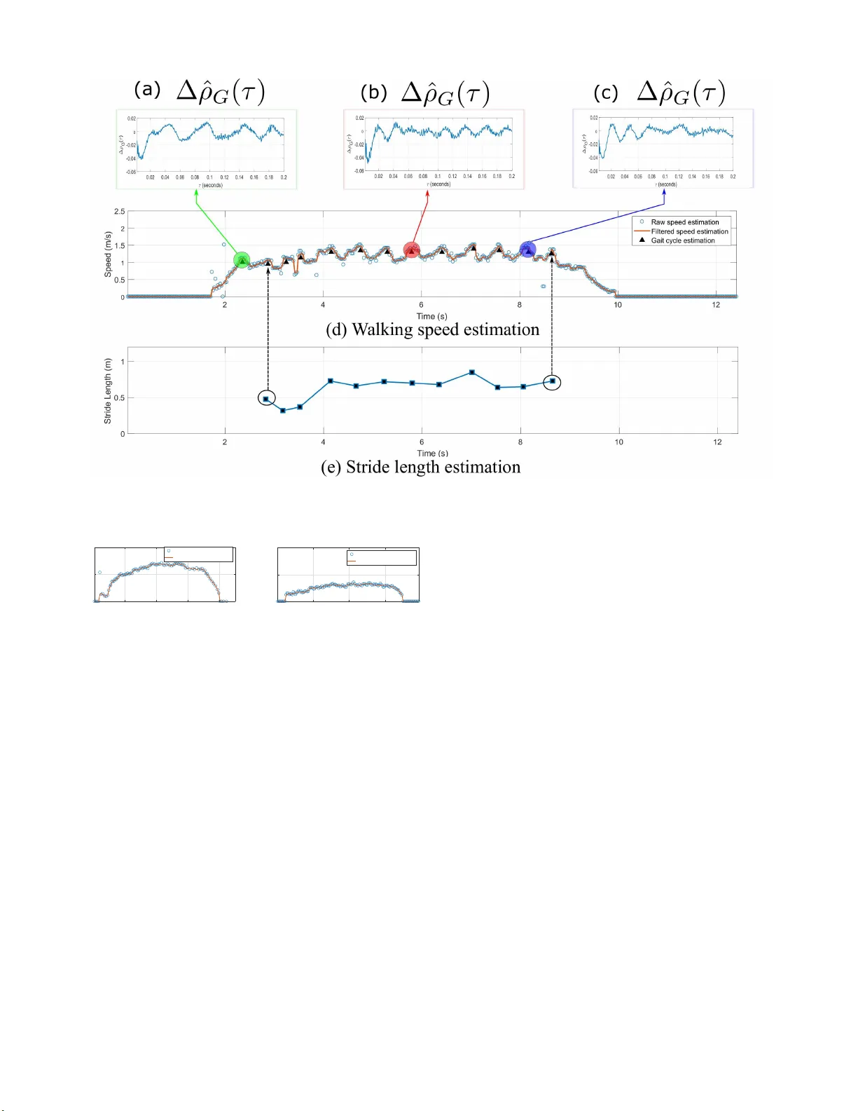
Leave a Comment